Bayesian Classification and Change Point Detection for Functional Data.

(1)

ABSTRACT

LI, XIUQI. Bayesian Classification and Change Point Detection for Functional Data. (Under the direction of Subhashis Ghoshal).

In the first part of the dissertation, we propose a Bayesian approach to estimat-ing parameters in multiclass functional models. Unordered multinomial probit, ordered multinomial probit and multinomial logistic models are considered. We use finite ran-dom series priors based on a suitable basis such as B-splines in these three multinomial models, and classify the functional data using the Bayes rule. We average over models based on the marginal likelihood estimated from Markov Chain Monte Carlo (MCMC) output. Posterior contraction rates for the three multinomial models are computed. We also consider Bayesian linear and quadratic discriminant analyses on the multivariate data obtained by applying a functional principal component technique on the original functional data. A simulation study is conducted to compare these methods on different types of data. We also apply these methods to phoneme dataset.

(2)

(3)

(4)

Bayesian Classification and Change Point Detection for Functional Data

by Xiuqi Li

A dissertation submitted to the Graduate Faculty of North Carolina State University

in partial fulfillment of the requirements for the Degree of

Doctor of Philosophy

Operations Research

Raleigh, North Carolina 2018

APPROVED BY:

Sujit Ghosh Arnab Maity

Negash Medhin Subhashis Ghoshal

(5)

DEDICATION

(6)

BIOGRAPHY

(7)

ACKNOWLEDGEMENTS

I would like to express my deepest and sincerest gratitude to my advisor Dr. Subhashis Ghoshal for his great guidance, patience, and expertise. This dissertation would not have been possible without his advice and support.

I am very grateful to Dr. Sujit Ghosh, Dr. Arnab Maity, and Dr. Negash Medhin for their serving on my committee, with additional thanks to Dr. Sujit Ghosh for his serving as the graduate school representative. I appreciate their valuable comments and suggestions for my research and presentation.

I am also very grateful to the faculty and staff of Operations Research Program and Statistics Department. Especially, I would like to thank Dr. Negash Medhin for his help to find funding for me. I would like to thank Ms. Linda Smith and Ms. Lanakila Alexander for their help. I also want to thank Dr. Ana–Maria Staicu for her time and valuable advice.

Special thanks to all my friends who always support and encourage me.

(8)

LIST OF TABLES

Table 2.1 Averaged misclassification rates for simulated data . . . 38 Table 2.2 Averaged misclassification rates for 3-class phoneme data . . . 42 Table 2.3 Estimate and standard error of the posterior mean for the 3-class

or-dered multinomial model (J = 6) . . . 42 Table 2.4 Estimate and standard error of the posterior mean for the 3-class

multi-nomial logistic model (J = 10) . . . 43 Table 2.5 Estimate and standard error of the posterior mean for the 3-class

un-ordered multinomial model (J = 14) . . . 43 Table 2.6 Averaged misclassification rates for 5-class phoneme data . . . 44 Table 2.7 Estimate and standard error of the posterior mean for the 5-class

un-ordered multinomial model (J = 14) . . . 46 Table 2.8 Estimate and standard error of the posterior mean for the 5-class

multi-nomial logistic model (J = 14) . . . 47 Table 2.9 Estimate and standard error of the posterior mean for the 5-class

(11)

LIST OF FIGURES

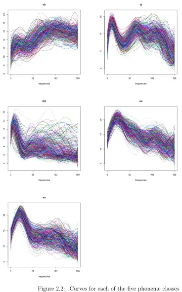
Figure 2.1 Coefficient functions for the multinomial models . . . 36 Figure 2.2 Curves for each of the five phoneme classes . . . 40 Figure 2.3 γ2 sampled from Metropolis-Hastings when J=5–7 and 13–15 . . . . 42 Figure 2.4 γ2,γ3, andγ4 sampled from Metropolis-Hastings whenJ=5, 10, 15 . 45 Figure 3.1 Land-surface average temperature curves between 1753–2016 . . . 72 Figure 3.2 Land-surface average temperature curves for every 66 years . . . 74 Figure 3.3 C(k) for different k between 1753–2016 . . . 75 Figure 3.4 The plot on the left is the land-surface average temperature curves

between 1753–1913. The plot on the right is the land-surface average temperature curves between 1914–2016. . . 75 Figure 3.5 C(k) for different k between 1753–1913 . . . 76 Figure 3.6 The plot on the left is the land-surface average temperature curves

between 1753–1838. The plot on the right is the land-surface average temperature curves between 1839–1913. . . 76 Figure 3.7 C(k) for different k between 1914–2016 . . . 77 Figure 3.8 The plot on the left is the land-surface average temperature curves

(12)

Chapter 1 Introduction

Functional data analysis (FDA) deals with the analysis of data occurring in the form of functions. Wang et al. (2016) gave an overview of FDA including functional principal component analysis, functional linear regression, clustering and classification of functional data. FDA is increasingly drawing attention in many areas, such as biomedicine, envi-ronmental studies, and economics (Ullah and Finch, 2013). Mallor, Moler, and Urmeneta (2017) proposed a model based on functional principal component analysis to predict household electricity consumption. Wagner-Muns et al. (2018) proposed a method that uses functional principal components analysis to forecast traffic volume.

(13)

pro-posed a functional segment discriminant analysis (FSDA), which combines the classical linear discriminant analysis and support vector machines. Wavelets approaches are also applied to classify and cluster functional data (Ray and Mallick, 2006; Antoniadis et al., 2013; Chang, Chen, and Ogden, 2014; Suarez and Ghosal, 2016). There are also non-parametric approaches for functional data classification (Biau, Bunea, and Wegkamp, 2005; Ferraty and Vieu, 2003). Mosler and Mozharovskyi (2017) introduced a nonpara-metric procedure that transformed the original functional data into the DD-plot through a two-step transformation, and hence the classification operated on a low-dimensional space. Delaigle and Hall (2013) introduced methods to classify the functional data not observed on the same interval. Lee, Shin, and Lee (2016) proposed a logistic regression for functional data classification that is robust to misdiagnosis or label noise. Epifanio (2008) proposed several shape descriptors for classifying functional data. Alonso, Casado, and Romo (2012) proposed a method based on the distances from the observation or its derivatives to group representative functions for discriminating functional data. Nguyen, McLachlan, and Wood (2016) developed a method to classify bivariate functional data by combining the current techniques in spatial spline regression with finite mixture mod-els and mixed-effects modmod-els. Chamroukhi, Glotin, and Sam´e (2013) proposed a mixture discriminant analysis approach based on hidden process regression to handle the problem of complex-shaped classes of curves, where each class is potentially composed of several sub-classes.

(14)

among multiple functional predictors. Stingo, Vannucci, and Downey (2012) proposed a Bayesian conjugate normal discriminant model on the wavelet transform of the functional data. Zhu, Brown, and Morris (2012) introduced two Bayesian approaches: the Gaussian, wavelet-based functional mixed model and the robust, wavelet-based functional mixed model.

In Chapter 2, we propose a Bayesian approach to estimating parameters in multi-class functional models. Unordered multinomial probit, ordered multinomial probit and multinomial logistic models are considered. We use finite random series priors based on a suitable basis such as B-splines in these three multinomial models, and classify the functional data using the Bayes rule. We average over models based on the marginal likelihood estimated from Markov Chain Monte Carlo (MCMC) output. Posterior con-traction rates for the three multinomial models are computed. We also consider Bayesian linear and quadratic discriminant analyses on the multivariate data obtained by applying a functional principal component technique on the original functional data. A simulation study is conducted to compare these methods on different types of data. We also apply these methods to a phoneme dataset.

(15)

on Hilbert space theory and critical values are deduced from bootstrap iterations. Aue, Rice, and S¨onmez (2018) proposed a method to uncover structural breaks in functional data that does not rely on dimension reduction techniques.

(16)

Chapter 2 Bayesian Classification of Multiclass

Functional Data

2.1 Introduction

(17)

for functional data classification (Biau, Bunea, and Wegkamp, 2005; Ferraty and Vieu, 2003). However, there are only a few approaches proposed in the context of Bayesian classification for functional data. Wang, Ray, and Mallick (2007) developed a Bayesian hierarchical model which combines the adaptive wavelet-based function estimation and the logistic classification. Zhu, Vannucci, and Cox (2010) proposed a Bayesian hierarchi-cal model that takes into account random batch effects and selects effective functions among multiple functional predictors. Stingo, Vannucci, and Downey (2012) proposed a Bayesian conjugate normal discriminant model on the wavelet transform of the functional data. Zhu, Brown, and Morris (2012) introduced two Bayesian approaches: the Gaussian, wavelet-based functional mixed model and the robust, wavelet-based functional mixed model.

In this chapter, we consider a responseY taking valuesk = 1, . . . , K, with functional covariate{X(t), t∈[0,1]}. The main problem is to estimate the probability P(Y =k|X), which can be conveniently modeled by a function of R β(t)X(t)dt

P(Y =k|X) = Hk

Z

β(t)X(t)dt

, (2.1)

where Hk is a cumulative distribution function, and β(·) is an unknown (possibly vector

of) coefficient function(s). Unordered multinomial probit, ordered multinomial probit and multinomial logistic models are considered in this chapter which correspond to different choices ofHk, k= 1, . . . , K. For an ordered multinomial probit model, there are additional

(18)

of the parameters are obtained using the training data, and then the classification rules are applied to the test data using the posterior probability of class membership.

The primary goal of a basis expansion method is to reduce a more complex problem to a simpler problem which has either a known solution or is likely to be easier to solve. A prior on function through finite random series is a standard tool in nonparametric Bayesian inference, but in the context of functional data, the technique has not been utilized to its fullest potential, especially regarding the study of theoretical property of Bayesian methods. Only one paper (Shen and Ghosal, 2015) has one example of functional linear regression treated using finite random series priors. We take that idea but develop it in the context of functional data classification. Characterizing contraction rate is a major goal of this chapter. For this, we need to estimate the complexity of the model and the prior concentration. Even though, the model reduces to the finite dimensional setting from the computational point of view, the effect of the residual bias in the approximation of function must be properly addressed. Hence the treatment substantially different from that of a parametric problem. In particular, the dimension of the basis must be adapted with the smoothness and the sample size by using a prior on it.

(19)

2.2 Model

2.2.1 Ordered Multinomial Probit Model

Let Xi(t), i = 1, . . . , n, t ∈ [0,1], be the orbserved functional data associated with a

categorical variable Yi taking possible values 1, . . . , K. We assume that (Xi, Yi), i =

1, . . . , n, are independent and identically distributed (i.i.d) observations.

Following Albert and Chib (1993), we consider the model described implicitly as fol-lows: there exists a latent variableWi distributed as N(

R

β(t)Xi(t)dt,1), fori= 1, . . . , n,

and that Yi = k if γk−1 < Wi ≤ γk, where k = 1, . . . , K. The latent variables Wi,

i= 1, . . . , n, are independent. The coefficient function β(·) is unkown. The cut-points γk

are also unknown except that γ0 = −∞ and γK = ∞. To ensure identifiability, we set

γ1 = 0. Under the assumed model, the probability of choosing a category k is given by

P(Yi =k|Xi) = Φ

γk−

Z

β(t)Xi(t)dt

−Φ

γk−1− Z

β(t)Xi(t)dt

, (2.2)

where Φ stands for the distribution function of the standard normal distribution.

2.2.2 Unordered Multinomial Probit Model

Let Xi(t), i = 1, . . . , n, be the same as in the Section 2.2.1, and also same for Section

2.2.3.

The unordered multinomial probit model can be described by the following data augmentation method. As in Albert and Chib (1993), let W_i0 = (W_i0₁, . . . , W_iK0 )T, i = 1, . . . , n, be latent variable, such that W_il0 follows a linear model

W_il0 = Z

(20)

where ε0_il ∼ N(0,1), i = 1, . . . , n, l = 1, . . . , K, are i.i.d. standard normal random vari-ables. Consider the latent variablesWi = (Wi1, . . . , WiK−1)T, Wil =Wil0 −W

0

iK,

Wil =

Z

β_l0(t)Xi(t)dt−

Z

β_K0 (t)Xi(t)dt+εil, (2.4)

where εil = ε0il −ε

0

iK, and l = 1, . . . , K −1. Let εi = (εi1, . . . , εiK−1)T. Then εi follows

N(0,Σ), where Σ is a (K−1)×(K−1) matrix with 2 at diagonal entries and 1 at all off-diagonal entries.

The probability of choosing the kth (k= 1, . . . , K−1) alternative is given by

P(Yi =k|Xi) = P(Wik > Wil, for alll6=k,andWik >0), (2.5)

and the probability of choosing alternative K is given by

P(Yi =K|Xi) = P(Wil <0 for alll = 1, . . . , K −1). (2.6)

2.2.3 Multinomial Logistic Model

In this model, the probability of choosing category k is given by

P(Yi =k|Xi) =

expR βk(t)Xi(t)dt

PK

l=1exp R

βl(t)Xi(t)dt

. (2.7)

To ensure model identification, set βK(t) = 0. Then the probability of choosing

cate-goty k (k = 1, . . . , K−1) is given by

P(Yi =k|Xi) =

expR

βk(t)Xi(t)dt

1 +PK−1

l=1 exp R

βl(t)Xi(t)dt

(21)

and the probability of choosing category K is given by

P(Yi =K|Xi) =

1 1 +PK−1

l=1 exp R

βl(t)Xi(t)dt

. (2.9)

2.3 Finite Random Series Prior

The functional coefficientβ(t) (or β1(t), . . . , βK(t) for unordered multinomial probit and

multinomial logistic models) is given a prior which is a finite linear combination of a certain chosen basis functions: β(t) = PJ

j=1θjψj(t), where {ψ1(t), . . . , ψJ(t)} is a basis, for example, formed by B-splines, Fourier functions, or wavelets. A prior is put on the unknown coefficients (θ1, . . . , θJ). The number of basis function J is also unknown and

should be given a hyperprior. Instead of sampling across the different dimensions using reversible jump MCMC (Green, 1995) which has computational difficulty for complicated models, we can implement MCMC for a givenJ value, and repeat it for relevantJ values. Thus, we can compute the marginal likelihood m(Y|J) for potentially interesting values of J, and obtain the posterior probability of J, which are discussed in Section 2.4.

The advantage of a using finite random series prior is that the inner product between the functional coefficient and the functional data R β(t)Xi(t)dt is reduced to a simple

linear combination

Z

β(t)Xi(t)dt =

Z J X

j=1

θjψj(t)Xi(t)dt= J

X

j=1

θjZij, (2.10)

where Zij =

R

(22)

2.3.1 Ordered Multinomial Probit Model

Using a finite random series β(t) = PJ

j=1θjψj(t), the model in (2.2) can be rewritten as

P(Yi =k|Xi) = Φ γk− J

X

j=1

θjZij

!

−Φ γk−1 −

J

X

j=1

θjZij

!

, (2.11)

where Zij =

R

ψj(t)Xi(t)dt.

Define θ = (θ1, . . . , θJ)T, and Zi = (Zi1, . . . , ZiJ)T. Then (2.11) can be written

com-pactly as

P(Yi =k|Xi) = Φ(γk−ZiTθ)−Φ(γk−1−ZiTθ). (2.12)

Clearly the unobserved latent variable Wi follows NJ(ZiTθ,1), where NJ stands for the

J-variate normal distribution. Assign a conjugate prior θ ∼NJ(θ0, B0), whereθ0 isJ×1 mean vector, and B0 is a J×J covariance matrix. Then the posterior distribution of θ is given by

θ|Y, W ∼NJ(θn, Bn), Bn= (B0−1+Z

T_Z₎−1_{, θ}

n =Bn(B0−1θ0+ZTW), (2.13)

where Z = (ZT

1 , . . . , ZnT)T, and W = (W1, . . . , Wn)T.

We follow the scheme introduced by Albert and Chib (1993). The posterior distribu-tion of Wi is given by

Wi|(θ, γ, Yi =k)∼TN(ZiTθ,1, γk−1, γk), (2.14)

(23)

mean ZT

i θ, and variance 1 to the interval (γk−1, γk).

Albert and Chib (1993) assigned a diffuse prior on the cut-points. However, model averaging needs a proper prior. A normal prior is not appropriate due to the order restriction on γ1, . . . , γK. Albert and Chib (1997) proposed a transformation of γ =

(γ1, . . . , γK) which avoids the order restriction.

α1 = logγ2, αj = log(γj+1−γj), 2≤j ≤K −2. (2.15)

Note that γ1 = 0 and by the inverse map

γj = j−1 X

l=1

eαl_, ₂_≤_j _≤_K₋₁_. _(2.16)

Then γ can be reparameterized by α = (α1, . . . , αK−2). Assign a multivariate normal prior with mean α0, and covariance A0 on α. To sample γ, apply the following steps of Metropolis-Hastings algorithm.

1. Sample α0 from a proposal distributionq(α0, α|Y, θ, W). Here we allow the proposal density to depend on the data and the two remaining blocks for the convenience of computing the marginal likelihood in the future.

2. Move to α0 from the currentα with probability

ρ(α, α0|Y, θ, W) = minnf(Y|α

0_{, θ, W}₎_π₍_α0_{, θ}₎

f(Y|α, θ, W)π(α, θ)

q(α0, α|Y, θ, W)

q(α, α0_{|Y, θ, W}₎,1 o

. (2.17)

3. Compute γ by the inverse map (2.16).

(24)

The values of γ sampled from the Metropolis-Hastings algorithm converges quickly. We demonstrate it on the real data in Section 2.8 by plotting the sampling values of γ.

2.3.2 Unordered Multinomial Probit Model

Letβ_l0(t) =PJ

j=1θ 0

ljψj(t), where l = 1, . . . , K. Then (2.4) can be rewritten as

Wil = J

X

j=1

θ0_ljZij − J

X

j=1

θ_Kj0 Zij +il = J

X

l=1

(θ_jl0 −θ0_jK)Zij +εil, (2.18)

where Zij =

R

ψj(t)Xi(t)dt.

Let θlj = θlj0 − θ

0

Kj, where j = 1, . . . , J. Define θl = (θl1, . . . , θlJ)T, and Zi =

(Zi1, . . . , ZiJ)T. Then (2.18) is given by

Wil =ZiTθl+εil, (2.19)

where i= 1, . . . , n, l= 1, . . . , K−1.

Define a J×(K−1) matrix Θ = (θ1, . . . , θK−1). Then we haveWi =ZiTΘ +εi, where

Wi = (Wi1, . . . , WiK−1)T,εi = (εi1, . . . , εiK−1)T, and εi ∼N(0,Σ).

In the model described in Section 2.2, Σ is known with 2 on diagonal entries and 1 on all off-diagonal entries. The only parameter needs to be estimated is Θ. In order to draw the matrix Θ using the Gibbs sampling, we can stack the data in a matrix form which is given by

W =ZΘ +ε, (2.20)

where W = (WT

(25)

matrix, and ε= (εT

1, . . . , εTn)T is an n×(K−1) matrix.

This results in a matrix normal distribution. The density function of matrix normal distribution MNn×p(M, U, V) is

(2π)−np/2|V|−n/2|U|−p/2exp

−1

2tr[V −1

(X−M)TU−1(X−M)]

, (2.21)

where M is an n ×p mean matrix, U is an n ×n row variance matrix, V is a p×p

column variance matrix, tr stands for the trace of a matrix, and |U| and |V| denote the determinants of U and V respectively.

Thus W|Θ ∼ MNn×(K−1)(ZΘ, In,Σ). Here the row variance-covariance matrix In

is an identity matrix of rank n, since W1, . . . , Wn are independent. We consider the

matrix normal prior Θ ∼ MNJ×(K−1)(U0, V0,Σ). By a standard conjugacy calculation, the posterior is given by

Θ|Y, W ∼MNJ×(K−1)(Un, Vn,Σ),

Vn = (ZTZ +V0−1) −1

, Un=Vn(ZTW +V0−1U0).

(2.22)

To draw a sample of W, we use the method introduced by McCulloch and Rossi (1994). Let Wi,−l denote (Wi1, . . . , Wi,l−1, Wi,l+1, . . . , WiK−1)T, Zi,· denote the ith row of

Z, the vector Θ·,l denote the lth column of Θ, the matrix Θ·,−l denote Θ without the

lth column, the scalar Σl,l denote the (l, l)th entry of Σ, Σ−l,−l denote Σ without the

lth row and the lth column, Σ−l,l denote the lth column of Σ without the lth entry, and

Σl,−l denote the lth row of Σ without the lth entry. We draw Wil from the conditional

(26)

(a, b) described below:

Wil|(Wi,−l,Θ, Yi)∼TN(mil, τil2, a, b),

mil =Zi,·Θ·,l+ ΣT−l,lΣ

−1

−l,−l(Wi,−l−Zi,·Θ·,−l),

τ_il2 = Σl,l−Σl,−lΣ−1−l,−lΣ−l,l,

(a, b) =               

(max{Wi,−l,0},∞), if Yi =l, l= 1, . . . , K −1,

(−∞,max{Wi,−l}), if Yi 6=l, l= 1, . . . , K −1,

(−∞,0), if Yi =K,

i= 1, . . . , n, l = 1, . . . , K −1.

(2.23)

To implement the Gibbs sampling, we draw samples from (2.22) and (2.23).

2.3.3 Multinomial Logistic Model

Letβk(t) = P_jJ₌₁θkjψj(t). Then (2.8) and (2.9) can be rewritten as

P(Yi =k|Xi) =

exp h

PJ

j=1θkjZij i

1 +PK−1

l=1 exp h

PJ

j=1θljZij

i, k = 1, . . . , K −1, (2.24)

P(Yi =K|Xi) =

1 1 +PK−1

l=1 exp h

PJ

j=1θljZij

i, (2.25)

where Zij =

R

ψj(t)Xi(t)dt.

Define θk = (θk1, . . . , θkJ)T,k = 1, . . . , K −1, and Zi = (Zi1, . . . , ZiJ)T. Then (3.24)

and (3.25) are given by

P(Yi =k|Xi) =

expZ_iTθk

1 +PK−1

l=1 exp[ZiTθl]

(27)

P(Yi =K|Xi) =

1 1 +PK−1

l=1 exp[ZiTθl]

. (2.27)

For each θk,k = 1, . . . , K−1, we assign a multivariate normal prior NJ(µk,Σk), and

apply Metropolis-Hastings algorithm to sample θk.

1. Sample θ0_k from the proposal distribution q(θ0_k, θk|Y, θ−k).

2. Move to θ_k0 from the current θk with probability

ρ(θk, θk0|Y, θ−k) = min

nf(Y|θ0

k, θ−k)π(θk0, θ−k)

f(Y|θk, θ−k)π(θk, θ−k)

q(θ_k0, θk|Y, θ−k)

q(θk, θ_k0|Y, θ−k)

,1o, (2.28)

where θ−k denotes all the blocks except the kth one.

2.4 Marginal Likelihood and Model Averaging

In Section 2.3, we described the MCMC sampling technique for a given J value, which we need to repeat it for all possible J values. In the actual computation, however, it is impossible to consider all values ofJ. With a given prior onJ, for example, geometric or Poisson distribution, the posterior probabilities for very small or very large values of J

decay to zero very quickly. Thus, we do not need to consider theseJ values. LetJ1, . . . , JS

denote the values ofJ we need to consider. If we can get the marginal likelihoodm(Y|Js),

then we can compute the posterior probability of Js using Bayes’s rule

P(Js|Y) =

m(Y|Js)p(Js)

PS

l=1m(Y|Jl)p(Jl)

, (2.29)

(28)

For each given Js, we have a misclassification rate rs, which is defined as the ratio of

the number of falsely classified data to the total number of data. Then we can obtain the average misclassification rate ¯r for each multinomial model:

¯

r =

S

X

s=1

P(Js|Y)·rs. (2.30)

We call it the model averaging method.

The marginal likelihood can be written as the normalizing constant of the posterior density

m(Y|Js) =

f(Y|Js, B)π(B|Js)

π(B|Y, Js)

, (2.31)

where B is a convenient value of the parameter in the context of the support of the posterior distribution such as the posterior mean, because (2.31) holds for any B. The numerator is the product of the likelihood and the prior. The denominator is the posterior density of B. For a given B∗, the posterior density π(B∗|Y, Jm) can be estimated from

the Gibbs output (Chib, 1995) and the Metropolis-Hasting output (Chib and Jeliazkov, 2001). Then the estimated marginal likelihood in the logarithm scale is

log ˆm(Y|Js) = logf(Y|Js, B∗) + logπ(B∗|Js)−log ˆπ(B∗|Y, Js). (2.32)

(29)

2.4.1 Ordered Multinomial Probit Model

There are two parameter blocks in this model,θ andα, whereα is the transformation of

γ as in (2.15). Given θ∗ =G−1PG

g=1θ

(g)_{, and} _α∗ ₌ _G−1PG

g=1α

(g)_{, where} _{θ(g)_{, α}(g)_}G g=1 are from the MCMC output, the joint posterior density can be written as

π(θ∗, α∗|Y, Js) =π(α∗|Y, Js)π(θ∗|Y, Js, α∗), (2.33)

where

π(θ∗|Y, Js, α∗) =

Z

π(θ∗|Y, Js, α∗, W)π(W|Y, Js, α∗)dW. (2.34)

The Monte Carlo estimate of π(θ∗|Y, Js, α∗) is

ˆ

π(θ∗|Y, Js, α∗) = M−1 M

X

m=1

π(θ∗|Y, Js, α∗, W(m)), (2.35)

where {W(m)_}M

m=1 are sampled from distribution [W|Y, Js, α∗]. The draws of W from

the Gibbs sampler are from the distribution [W|Y, Js], so π(θ∗|Y, Js, α∗, W) cannot be

averaged directly by the Gibbs sampling output. Addtional sampling for W is needed. We sample {θ(m)_} _{from the density} _π₍_{θ|Y, J}

s, α∗, W), and given that θ(m), we sample

{W(m)_} _from_π₍_W_{|Y, J}

s, θ, α∗).

The explicit distribution ofα∗ given (Y, Js) is unknown, and hence the draws ofα are

obtained from a Metropolis-Hastings sampling. By the local reversibility condition (see Chib and Jeliazkov (2001) for details), the posterior density of α can be written as

π(α∗|Y, Js) =

E1{ρ(α, α∗|Y, Js, θ, W)q(α, α∗|Y, Js, θ, W)}

E2{ρ(α∗, α|Y, Js, θ, W)}

(30)

whereρ(α, α∗|Y, Js, θ, W) is defined in (2.17),q(α, α∗|Y, Js, θ, W) is the proposal density,

the expectation E1 is with respect to the distribution π(θ, α, W|Y, Js), and E2 is with respect to the distributionπ(θ, W|Y, Js, α∗)×q(α∗, α|Y, Js, θ, W).

Then an estimate of π(α∗|Y, Js) is given by

G−1PG

g=1ρ(α

(g)_{, α}∗_{|Y, J}

s, θ(g), W(g))q(α(g), α∗|Y, Js, θ(g), W(g))

M−1PM

m=1ρ(α∗, α(m)|Y, Js, θ(m), W(m))

, (2.37)

where {θ(g)_{, α}(g)_{, W}(g)_}G

g=1 are obtained from the MCMC output. {θ(m), W(m)} are ob-tained fromπ(θ|Y, Js, α∗, W) and π(W|Y, Js, θ, α∗), and then given {θ(m), W(m)}, sample

α(m) _from_q₍_α∗_{, α|Y, J}

s, θ(m), W(m)).

2.4.2 Unordered Multinomial Probit Model

The only unknown parameter is Θ. For Θ∗ =G−1PG

g=1Θ

(g)_{, where} _{_Θ(g)_} _{are from the} Gibbs sampling output, the posterior density of Θ at Θ∗ can be written as

π(Θ∗|Y, Js) =

Z

π(Θ∗|Y, Js, W)π(W|Y, Js)dW. (2.38)

Then the Monte Carlo estimate of π(Θ∗|Y, Js) is

ˆ

π(Θ∗|Y, Js) = G

X

g=1

π(Θ∗|Y, Js, W(g)), (2.39)

where {W(g)_}G

g=1 are from the Gibbs sampling output.

(31)

Θ = (θ1, . . . , θK−1), where θl=θl0−θ

0

K,l = 1, . . . , K −1. Then (2.6) can be rewritten as

P(Y =K)

= 1

(2π)(K−1)/2_|_Σ_|1/2

Z −ZTΘ·,1 −∞

. . .

Z −ZTΘ·,K−1 −∞

exp − 1

2U

T_Σ−1

UdU,

(2.40)

where Θ·,l denotes the lth column of Θ.

For l6=K, let Θl _{= (}_θ

1−θl, . . . , θl−1−θl, θl+1−θl, . . . , θK−1−θl,−θl), then

P(Y =l)

= 1

(2π)(K−1)/2_|_Σ_|1/2

Z −ZTΘl·,1 −∞

. . .

Z −ZTΘl_·_,K₋₁ −∞

exp − 1

2U

T

Σ−1UdU.

(2.41)

Due to the exchangeable correlation structure of Σ, (2.41) can be reduced to a one dimensional integral (Dunnett, 1989) given by

P(Y =l) = √1

π Z ∞ 0 K−1 Y k=1

Φ(−u√2−ZTΘl·,k) + K−1

Y

k=1

Φ(u√2−ZTΘl·,k) e

−u2

du.

(2.42)

The expression in (2.40) can also be reduced to the same form as in (2.42). Then (2.42) can be approximated by Gaussian quadrature as follow

P(Y =l)≈ 1

2wq

K−1 Y

k=1

Φ(−p

2xq−ZTΘl·,k) + K−1

Y

k=1

Φ(p2xq−ZTΘl·,k) , (2.43)

where wq and xq are the weights and roots of the Laguerre polynomial of order Q.

(32)

2.4.3 Multinomial Logistic Model

There are K −1 unknown parameters: θ1, . . . , θK−1. Given θ∗_k = G−1PG_g₌₁θ(_kg), k = 1, . . . , K −1, where {θ_k(g)}G

g=1 are from the Metropolis-Hastings sampling output, the joint posterior density can be written as

π(θ₁∗, . . . , θ_K∗₋₁|Y, Js) = K−1

Y

i=1

π(θi|Y, Js, θ1∗, . . . , θ ∗

i−1). (2.44)

By the local reversibility, each full conditional density can be written as

π(θi|Y, Js, θ∗1, . . . , θ ∗

i−1) = E1{ρ(θi, θ

∗

i|Y, Js,Ψ∗i−1,Ψi+1)q(θi, θi∗|Y, Js,Ψ∗i−1,Ψi+1)} E2{ρ(θ∗i, θi|Y, Js,Ψ∗i−1,Ψi+1)}

,

(2.45)

where Ψi−1 = (θ1, . . . , θi−1), Ψi+1 = (θi+1, . . . , θK−1), ρ(θi, θ∗i|Y, Js,Ψ∗i−1,Ψi+1) is de-fined in (2.28), q(θi, θi∗|Y, Js,Ψ∗i−1,Ψi+1) is the proposal density, E1 is the expectaion with respect to the distribution π(θi,Ψi+1|Y, Js,Ψ∗i−1), and E2 is that with respect to

π(Ψi+1_{|Y, J}

s,Ψ∗i−1, θ∗i)×q(θ

∗

i, θi|Y, Js,Ψ∗i−1,Ψi+1). Then an estimate of π(θi|Y, Js, θ∗1, . . . , θ

∗

i−1) is given by

ˆ

π(θi|Y, Js, θ∗1, . . . , θ ∗

i−1) = G

−1PG

g=1ρ(θ (g)

i , θ

∗

i|Y, Js,Ψ∗i−1,Ψi+1,(g))q(θ (g)

i , θ

∗

i|Y, Js,Ψ∗i−1,Ψi+1,(g))

M−1PM

m=1ρ(θ ∗

i, θ

(m)

i |Y, Js,Ψ∗i−1,Ψi+1,(m))

,

(2.46)

where{θ(_ig),Ψi+1,(g)}G

g=1 are obtained fromπ(θi,Ψi+1|Y, Js,Ψ∗i−1).{Ψi+1,(m)}are obtained fromπ(Ψi+1|Y, Js,Ψ∗i−1, θi∗), and then for each{Ψi+1,(m)}, sampleθ

(m)

i fromq(θi∗, θi|Y, Js,

(33)

2.5 Posterior Contraction Rate

For classification problem, the most important object to study is the misclassification rate. By examining convergence to the true distribution, it follows that the Bayes pro-cedure has misclassification rate close to that of the oracle propro-cedure which uses the true values of the regression functions and other parameters (if any), e.g., cut-points in the ordered multinomial probit model. In the Bayesian nonparametric setting, Hellinger convergence is established by applying the general theory (Ghosal and van der Vaart, 2017). Thus, in this section, we only consider the contraction rate of the posterior dis-tribution with respect to a metric on the probability of categories, which is equivalent with Hellinger distance on the joint distribution. The posterior contraction rates of the three multinomial models with finite random series prior can be obtained using calcula-tion similar to those in Shen and Ghosal (2015) on posterior contraccalcula-tion rates for finite random series.

We use_.to denote an inequality up to a constant multiple,f gforf _.g _.f. For a vectorθ ∈_Rd_,_kθk

p ={Pd_i₌₁|θi|p}1/p, where 1≤p <∞, andkθk∞= max1≤i≤d|θi|.

Simi-larly, for a functionf with respect to a measure G, we definekfkp,G={

R

|f(x)|p_dG}1/p_,

where 1≤p < ∞, andkfk∞,G = supx|f(x)|. LetN(, T, d) denote the-covering number

of a set T for a metric d. Let h2₍_{p, q}_{) =} R

(√p−√q)2_dµ _{be the squared Hellinger} dis-tance, K(p, q) =R plog(p/q)dµ,V(p, q) =R plog2(p/q)dµbe the Kullback-Leibler (KL) divergences.

Suppose that (Xi, Yi),i= 1, . . . , n, are the independent observations. Letpdenote the

(34)

π0k be the true probablity of the kth category conditioned onX. Define the probability

vector π = (π1, . . . , πK)T, where πK = 1−PK

−1

k=1 πk, and π0 = (π01, . . . , π0K)

T_{, where}

π0K = 1−

PK−1

k=1 π0k. Assume that the distribution ofX isG, andν denotes the counting measure on{1, . . . , K}. For these multinomial models, the KL divergences K(p0, p), and

V(p0, p) can be reduced to

K(p0, p) = Z Z

p0(x, y) log

p0(x, y)

p(x, y) dν(y) dx =

Z Z

π0(y|x) logπ0(y|x)

π(y|x) dν(y) dG(x) = EX

n_XK

k=1

π0k(X) log

π0k(X)

πk(X)

o

=K(π0, π), say

(2.47)

V(p0, p) = Z Z

p0(x, y) log2

p0(x, y)

p(x, y) dν(y) dx =

Z Z

π0(y|x) log2

π0(y|x)

π(y|x) dν(y) dG(x) = EX

n_XK

k=1

π0k(X) log2

π0k(X)

πk(X)

o

=V(π0, π), say.

(2.48)

Similarly, the squared Hellinger distance h2(p1, p2) can be reduced to

h2(p1, p2) = Z Z

p

π1(y|x)− p

π2(y|x)

dν(y) dG(x)

= EX

n_XK

k=1 p

π1k(X)−

p

π2k(X)

2o

=h2(π1, π2), say.

(35)

We define a metric by

d(π, π0) = v u u t

K

X

k=1

EX|πk(X)−π0k(X)|2. (2.50)

Then we have the following slightly simplification of a general posterior contraction the-orem suitable in our context.

Theorem 1. Assume that π0 is bounded away from zero. Let n ≥ ¯n be two sequences

of positive numbers satisfying n →0and n¯n2 → ∞. Let X0 be such that P(X ∈X0) = 1 and πk(x), k = 1, . . . , K for x ∈ X0 is bounded away from 0. Let Wn be a subset of the

parameter space such that the following conditions hold for some positive constants a2

and a1 > a2+ 2:

logN(n,Wn, h).n2n, (2.51)

Π(π6∈Wn)≤exp{−a1n¯2n}, (2.52)

−log Π

K

X

k=1

kπk−π0kk2∞,X0 ≤¯2n

!

≤a2n¯2n, (2.53)

where kπk −π0kk∞,X0 = supx∈X0|πk(x)−π0k(x)|. Then for every Mn → ∞, we have

Π d(π, π0)≥Mnn|X(n), Y(n)

→0 in probability.

The proof follows from Theorem 4 of Ghosal and van der Vaart (2007a), by observing that

h2(π, π0) = EX K

X

k=1

|πk(X)−π0k(X)|2

|pπk(X) +

p

π0k(X)|2

&EX K

X

k=1

(36)

and by expanding in Taylor’s expansion

max{K(π0, π), V(π0, π)}.

K

X

k=1

kπk−π0kk2∞,X0. (2.55)

Let Π be a generic notation for priors on the number J of basis functions. As in Shen and Ghosal (2015), the priors on J and the coefficients of the basis functions θ = (θ1, . . . , θJ)T need to satisfy the conditons (A1) and (A2). For the ordered multinomial

probit model, we add condition (A3).

(A1) For some c1, c2 > 0, 0 ≤ t2 ≤ t1 ≤ 1, exp{−c1jlogt1j} ≤ Π(J = j) ≤ exp{−c2jlogt2j}.

(A2) Given J, Π(kθ −θ0k2 ≤ ) ≥ exp{−c3Jlog(1/)} for every kθ0k∞ ≤ H, where c3 is some positive constant, H is chosen sufficiently large, and > 0 is sufficiently small. Also, assume that Π(θ6∈[−M, M]J)≤Jexp{−CMt3_}_{for some cosntant}_C_,

t3 >0,

(A3) Given K categories, Π(kγ −γ0k2 ≤ ) ≥ exp{−c4Klog(1/)}, where c4 is some positive constant.

Geometric distribution with t1 = t2 = 0, and Poisson distribution with t1 = t2 = 1 on

J satisfy (A1). The multivariate normal distribution on θ and γ satisfy (A2) and (A3) respectively.

(37)

that

kβ0(·)−θT0ψ(·)kr .J−α, (2.56)

kθT

1ψ(·)−θ

T

2ψ(·)kr.JK0kθ1−θ2k2, θ1, θ2 ∈RJ. (2.57)

Remark 2 of Shen and Ghosal (2015) gave examples of bases satisfying relations (2.56) and (2.57). For B-splines, the relations hold whenK0 = 1/2 withr = 2, andK0 = 1 with

r=∞.

Remark 1. Parameter estimation plays a secondary role here. The problem of estimating model parameters is interesting in its own right but is not necessary for good classifica-tions. Cai and Hall (2006) and Yuan and Cai (2010) showed that the parameter function estimation and the prediction from an estimator of the parameter function have different characteristics.

2.5.1 Ordered Multinomial Probit Model

Letγ = (γ1, . . . , γK)T be the vector of the threshold points, and γ0 = (γ01, . . . , γ0K)T be

the vector of the true values of the threshold points. Let β(t) be the parameter function on [0,1], andβ0(t) be the true parameter function on [0,1]. Let

πk(X) = Φ

γk−

Z

β(t)X(t)dt−Φγk−1− Z

β(t)X(t)dt, (2.58)

and

π0k(X) = Φ

γ0k−

Z

β0(t)X(t)dt

−Φγ0k−1− Z

β0(t)X(t)dt

(38)

Theorem 2. Assume that kXk1 = R

|X(t)|dt is a bounded random variable, the pri-ors satisfy the conditons (A1), (A2) and (A3), and that the basis ψ(t) satisfies (2.56) and (2.57) with r =∞. Then the posterior contraction rate of the ordered multinomial probit model is n n−α/(2α+1)(logn)α/(2α+1)+(1−t2)/2 relative to d(π, π0). More explic-itly, for every Mn → ∞, Π(β : ρ(β, β0) ≥ Mnn|X(n), Y(n)) → 0 in probability, where

ρ(β, β0) = EX|

R

(β(t)−β0(t))X(t) dt|, and Π(γ : maxj|γj−γ0j| ≥Mnn|X(n), Y(n))→0

in probability.

Proof. For any x ∈ X0 = { R

|X(t)|dt ≤ M}, say, by the Lipschitz continuity of Φ, we have

|πk(x)−π0k(x)|.max

k |γk−γ0k|+

Z

(β(t)−β0(t)x(t)dt

.kγ−γ0k∞+kβ(·)−β0(·)k∞ Z

|x(t)|dt

.kγ−γ0k∞+kβ(·)−β0(·)k∞.

(2.60)

Observe that with the finite random series prior, the L∞-distance between β(·) and

β0(·) is bounded by

kβ(·)−β0(·)k∞=kθTψ(·)−θ₀Tψ(·) +θ₀Tψ(·)−β0(·)k∞

≤ kθT_ψ₍_·₎₋_θT

0ψ(·)k∞+kθ0Tψ(·)−β0(·)k∞.

(39)

Then we have

Π

K

X

k=1

≥Π(kγ−γ0k ≤¯n/

√

2)Π(kβ(·)−β0(·)k∞≤¯n/

√

2)

≥Π(kγ−γ0k ≤¯n/

√

2)Π(kθ−θ0k ≤¯n/(2

√

2 ¯Jn K0

))

&exp−Klog√2/¯n

exp−J¯nlog

2√2 ¯Jn

K0

/¯n

.

(2.62)

To satisfy the relation (2.53), we need ¯J−α

n .¯n and

Klog√2/¯n

+ ¯Jnlog

2√2 ¯Jn

K0

/¯n

.n¯2_n. (2.63)

Thus (2.63) leads to the conditions that ¯Jnlogn .n¯2n. Then we obtain the preliminary

contraction rate ¯n n−α/(2α+1)(logn)α/(2α+1), for ¯Jn(n/logn)1/(2α+1).

Using (2.60), we obtain

logN(n,Wn, h).logN(n,Wn,k · k∞).n2n. (2.64)

According to Theorem 2 of Shen and Ghosal (2015), to satify (2.64), we need

Jn{(K0+ 1) logJn+ logMn+C0logn} ≤n2n, (2.65)

for some positive constant C0. To satify (2.52), we need

bn¯2_n ≤Jnlogt2Jn, logJn+n¯2n ≤M t3

n , (2.66)

(40)

n1/(2α+1)_(log_n₎2α/(2α+1)−t2_{. Relation (5.65) implies that} _J

nlogn . n2n. As a result, the

posterior contraction rate is nn−α/(2α+1)(logn)α/(2α+1)+(1−t2)/2 relative to d(π, π0). Further, by Jensen’s inequality, we have

EX|πk(X)−π0k(X)|2 ≥

n

EX|πk(X)−π0k(X)|

o2

. (2.67)

Ifk= 1, by the mean value theorem and the uniform positivity of Φ on compact interval, then

EX|π1(X)−π01(k)|= EX

Φ(− Z

β(t)X(t)dt)−Φ(−

Z

β0(t)X(t)dt)

&EX

Z

β(t)X(t)dt−

Z

β0(t)X(t)dt . (2.68)

Hence if EX|π1(X)−π01(X)|2 is small, then EX

R

β(t)X(t)dt−R

β0(t)X(t)dt

is also small. Ifk = 2, we have

EX|π2(X)−π02(k)|= EX

Φ(γ2− Z

β(t)X(t)dt)−Φ(γ02− Z

β0(t)X(t)dt)

−Φ(−

Z

β(t)X(t)dt) + Φ(−

Z

β0(t)X(t)dt)

&EX

Φ(γ2− Z

β0(t)X(t)dt)

−EX

Φ(− Z

β(t)X(t)dt)−Φ(−

Z

β0(t)X(t)dt) . (2.69)

From (2.68), we know that EX

Φ(−

R

β(t)X(t)dt)−Φ(−R

β0(t)X(t)dt)

is small, and if EX|π2(X)−π02(X)|2 is small, then

EX

Φ(γ2− Z

β0(t)X(t)dt)

(41)

is also small. By the mean value theorem and the uniform positivity of Φ on compact interval, we have

EX

Φ(γ2− Z

β0(t)X(t)dt)

&EX

γ2−γ02− Z

β(t)X(t)dt+ Z

β0(t)X(t)dt

&|γ2−γ02| −EX

Z

β(t)X(t)dt−

Z

β0(t)X(t)dt . (2.71)

Hence |γ2−γ02| is small. Similarly, we can prove that |γk−γ0k| is small for any k.

2.5.2 Unordered Multinomial Probit Model

Note that by (2.42)

πk(X) =

1

√ π

Z ∞ 0

nKY−1

l=1

Φ(−z√2−

Z

βl(t)X(t)dt)

+

K−1 Y

l=1

Φ(z√2−

Z

βl(t)X(t)dt)

o

e−z2dz

(2.72)

|X(t)|dt is a bounded random variable, the priors satisfy the conditons (A1) and (A2), and that the basis ψ(t) satisfies (2.56) and (2.57) with r = ∞. Then the posterior contraction rate of the unordered multinomial probit model is n n−α/(2α+1)(logn)α/(2α+1)+(1−t2)/2 relative to d(π, π0).

Proof. For some M > 0, P(X0) = 1 forX0 ={ R

(42)

Lipschitz continuity of the function Φ, we have

|πk(x)−π0k(x)|.

Z

βk(t)x(t)dt−

Z

β0k(t)x(t)dt

. Z

|βk(t)−β0k(t)| |x(t)|dt

.kβk(·)−β0k(·)k∞.

(2.73)

The L∞-distance between βk(·) and β0k(·) is bounded by

kβk(·)−β0k(·)k∞=kθT_kψ(·)−θ₀T_kψ(·) +θT₀_kψ(·)−β0k(·)k∞

≤ kθT

kψ(·)−θ T

0kψ(·)k∞+kθ T

0kψ(·)−β0k(·)k∞.

(2.74)

Then we have

Π

K

X

k=1

≥Π

K

X

k=1

kβk(·)−β0k(·)k2∞≤¯2n

≥Π(kθk−θ0kk ≤¯n/(2

√ KJ¯n

K0 ))

&exp−J¯nlog

2√KJ¯n K0

/¯n

.

(2.75)

To satisfy the relation (2.53), we need ¯J−α

n .¯n and

¯

Jnlog

2√KJ¯n K0

/¯n

.n¯2_n. (2.76)

Thus (2.76) leads to the conditions that ¯Jnlogn .n¯2n. Then we obtain the preliminary

contraction rate ¯n n−α/(2α+1)(logn)α/(2α+1), for ¯Jn(n/logn)1/(2α+1).

Following the same arguments as (2.64)–(2.66), the posterior contraction rate is n

(43)

2.5.3 Multinomial Logistic Model

Let βk(t), k = 1, . . . , K − 1, be the coefficient functions on [0,1], and β0k(t),

k = 1, . . . , K −1, be the true coefficient functions on [0,1].

|X(t)|dt is a bounded random variable, the priors satisfy the conditons (A1) and (A2), and that the basis ψ(t) satisfies (2.56) and (2.57) with r = ∞. Then the posterior contraction rate of the multinomial logistic model is

n n−α/(2α+1)(logn)α/(2α+1)+(1−t2)/2 relative to d(π, π0).

Proof. The proof is similar to that of Theorem 3.

2.6 Discriminant Analysis

As a comparison to those multinomial models, we use Bayesian discriminant analysis to classify the functional data. Instead of modeling the class probability directly, the dis-criminant analysis uses Bayes’s rule to compute the marginal likelihood ofYi (Gelman et

al., 2013). The classical discriminant analysis applies only to multivariate data. For func-tional data, we can use certain orthogonal linear functions to determine the classification probabilities:

(fi1, . . . , fim)T =

Z

β1(t)Xi(t)dt, . . . ,

Z

βm(t)Xi(t)dt

T

(2.77)

Ideally these β1(t), . . . , βm(t) are unknown, but putting a prior on these functions

with identifiability restrictions is complicated. We instead consider β1(t), . . . , βm(t) to

(44)

the means and the covariance matrices be unknown. Then discriminant analysis can be applied to the m principal components.

2.6.1 Linear Discriminant Analysis

Linear discriminant analysis assumes that for each of the K category, the set of lin-ear function (f1, . . . , fm) follows a normal distribution with the same covarince matrix:

(fil1, . . . , film)T ∼N(µl,Σ), where µl is the population mean of category l, l = 1, . . . , K,

i= 1, . . . , nl, andnl is the number of data in categoryl. Then the probability of choosing

category k is given by

P(Yi =k|Xi) =

pk·φ(fik1, . . . , fikm;µk,Σ)

PK

l=1pl·φ(fil1, . . . , film;µl,Σ)

, (2.78)

where φ(f1, . . . , fm;µ,Σ) is the multivariate normal density function with mean µ and

covariace Σ, and pl, l= 1, . . . , K, are the probability of choosing category l.

The variables fil1, . . . , film are the m principal components of Xi(t) in categoty l,

where l = 1, . . . , K. Define fil = (fil1, . . . , film)T, where i = 1, . . . , nl, and PK_l₌₁nl = n.

To estimate the mean µl for each category l, and the common covariance Σ among

all categories, we use the conjugate normal-inverse-Wishart prior with hyperparameters (Gelman et al., 2013) for (µl,Σ)

Σ∼IWν0(Λ −1

0 ), µl|Σ∼N(µl0,Σ/κ0). (2.79)

Then the posterior distribution of (µl,Σ) can be obtained in the following order

Σ|Y ∼IWνn(Λ

−1

(45)

where νn =ν0+n, ¯fl=Pn_i₌₁l fil/nl, S=PK_l₌₁Pn_i₌₁l (fil−f¯l)(fil−f¯l)T,

Λn = Λ0 +S+

K

X

l=1

κ0nl

κ0 +nl

( ¯fl−µl0)( ¯fl−µl0)T, (2.81)

and

κn=κ0+n, µln=

κ0µl0+nlf¯l

κ0+nl

, l = 1, . . . , K. (2.82)

2.6.2 Quadratic Discriminant Analysis

Quadratic discriminant analysis is defined in a similar way, except that it has a different covariance matrix for each category. The probability of choosing category k is given by

P(Yi =k|Xi) =

pk·φ(fik1, . . . , fikm;µk,Σk)

PK

l=1pl·φ(fil1, . . . , film;µl,Σl)

. (2.83)

To estimate the meanµland the covariance Σlfor each categoryl, wherel= 1, . . . , K,

we use the conjugate normal-inverse-Wishart prior with hyperparameters for (µl,Σl)

Σl ∼IWνl0(Λ −1

l0 ), µl|Σl∼N(µl0,Σl/κl0), (2.84)

for l = 1, . . . , K. Then the posterior distribution of (µl,Σl) can be obtained in the

following order

Σl|Y ∼IWνln(Λ

−1

(46)

where νln =νl0+nl, ¯fl =Pn_i₌₁l fil/nl, Sl =Pn_i₌₁l (fil−f¯l)(fil−f¯l)T,

Λln= Λl0+Sl+

κl0nl

κl0+nl

( ¯fl−µl0)( ¯fl−µl0)T, (2.86)

and

κln =κl0+nl, µln=

κl0µl0+nlf¯l

κl0+nl

, l = 1, . . . , K. (2.87)

2.7 Simulation

2.7.1 Data Generation

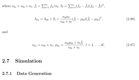
The simulated data are generated following different data generating process. All of the simulated data have three categories. In all cases considered below, we generate the functional data from a Gaussian process at discrete time points 0, 0.01,. . ., 0.99, 1, with the mean function sintand variation kernel 100 exp{−100(ti−tj)2}, whereti and tj were

the discrete time point 0, 0.01, . . ., 0.99, 1.

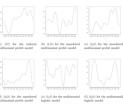
For the ordered multinomial probit data, the coefficient function β(t) is plotted in Figure 1 (a), and the four threshold points are chosen to be −∞, 0, 8, ∞. The four cut-off points construct three intervals. If the inner product of a functional data and the coefficient function plus a standard normal variable falls in the kth interval (γk−1, γk),

then the functional data attributes to the category k.

(47)

(a) β(t) for the ordered multinomial probit model

(b) β1(t) for the unordered

multinomial probit model

(c) β2(t) for the unordered

(d) β3(t) for the unordered

(e)β1(t) for the multinomial

logistic model

(f)β2(t) for the multinomial

logistic model

(48)

functional data belonges to the category with the largest sampled value.

For the multinomial logistic data, the coefficient functions β1(t), β2(t) are plotted in Figure 1 (e)–(f), and the third coefficient function β3(t) can be assumed to be zero everywhere. We compute the probability of a functional data falling into each category. Then the data attributes to the category with the largest probability.

For data satisfying the assumption of the linear discriminant analysis, we generate them from three Gaussian processes with different mean functions sint + 2 cost, sint, and sint−3 cost, but the same variation kernel exp{−30(ti−tj)2}.

For data satisfying the assumption of the quadratic discriminant analysis, we generate them from three Gaussian processes with different mean functions and different variation kernels. The mean functions are sint+ 2 cost, sint, and sint−3 cost, and the variation kernels are exp{−2 sin2(π(ti−tj))}, exp{−30(ti−tj)2}, and exp{−|ti−tj|}, respectively.

In this simulation study, we generate total 900 (300 for each category) functional data for each type of dataset. We constructe the training data with 720 (240 for each category) of them and the testing data with the remaining 180 (60 for each category) of them.

2.7.2 Basis Functions

(49)

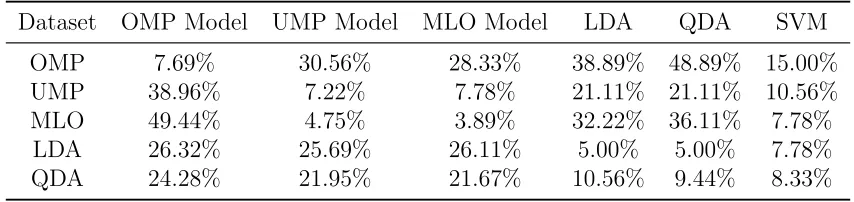
Table 2.1: Averaged misclassification rates for simulated data

Dataset OMP Model UMP Model MLO Model LDA QDA SVM

OMP 7.69% 30.56% 28.33% 38.89% 48.89% 15.00%

UMP 38.96% 7.22% 7.78% 21.11% 21.11% 10.56%

MLO 49.44% 4.75% 3.89% 32.22% 36.11% 7.78%

LDA 26.32% 25.69% 26.11% 5.00% 5.00% 7.78%

QDA 24.28% 21.95% 21.67% 10.56% 9.44% 8.33%

2.7.3 Results

Under the chosen models, we apply Baysian estimation methods described in Section 3 on the training data. In this study, 5000 MCMC iterations are obtained, and the first 1000 of them are discarded as burn-in. We use the last 4000 MCMC output of the parameter B to classify the 180 transformed testing data, where B = (θ, γ2, γ3) for the ordered multinomial probit model, B = Θ for the unorederd multinomial probit model,

B = (θ1, θ2) for the logistic model,B = (µ1, µ2, µ3,Σ) for the linear discriminant analysis model, and B = (µ1, µ1, µ3,Σ1,Σ2,Σ3) for the quadratic discriminant analysis model. A transformed testing data zi or fi is in categoty k if

P4000

g=1 1(Yi = k|zi or fi, B(g)) >

P4000

g=1 1(Yi = l|zi or fi, B

(50)

2.8 Application on Phoneme Data

Ferraty and Vieu (2006) extracted a speech recognition data originally introduced by a collaboration between Andreas Buja, Werner Stuetzle and Martin Maechler, and illus-trated in the paper by Hastie, Buja, and Tibshirani (1995). The dataset has five speech frames corresponding to the following five phonemes:

1. “sh” as in “she”;

2. “iy” as in “she”;

3. “dcl” as in “dark”;

4. “aa” as in “dark”;

5. “ao” as in “water”.

(51)

(52)

2.8.1 Three Classes

From Figure 2.2, we can see that class “aa” and “ao” have a very similar pattern which can cause difficulty in classification. To simplify the problem, in the beginning, we only classify the first three classes (“sh”, “iy”, and “dcl”). For computational efficiency, we only use 900 of them from three categories. We split the data into training and testing set by randomly sampling from each class, and keeping the same percentage of samples of each class as the complete set. The size of the testing data is 20% of the total data size. That is we have 240 data for each class in the training set, and 60 data for each class in the testing set. We put a geometric prior with p = 0.5 on J, and it is enough for us to consider the number of B-spline basis functions to be J = 5, . . . ,15. We obtain 5000 MCMC iterations and discard the first 1000 of them as burn-in.

(53)

(a)J = 5 (b)J = 6 (c)J = 7

(d)J = 13 (e)J = 14 (f) J = 15

Figure 2.3: γ2 sampled from Metropolis-Hastings whenJ=5–7 and 13–15 Table 2.2: Averaged misclassification rates for 3-class phoneme data

OMP Model UMP Model MLO Model LDA QDA

9.84% 0.56% 5.56% 7.78% 5.00%

Table 2.3: Estimate and standard error of the posterior mean for the 3-class ordered multinomial model (J = 6)

γ2 θ

(54)

Table 2.4: Estimate and standard error of the posterior mean for the 3-class multinomial logistic model (J = 10)

θ2

Estimate (13.10,18.25,6.04,−15.29,15.52,1.30,−5.81,4.65,−28.24,−16.91) Standard error (0.94,1.08,0.64,0.63,0.75,0.66,0.37,0.48,0.70,1.03)

θ3

Estimate (39.42,34.30,−3.47,5.26,−7.36,0.38,−17.99,−4.43,−11.23,2.44) Standard error (1.21,1.44,0.42,0.31,1.08,0.27,0.53,0.33,0.93,0.32)

Table 2.5: Estimate and standard error of the posterior mean for the 3-class unordered multinomial model (J = 14)

estimate standard error

Θ                        

−15.40 49.92 35.78 79.79 45.94 32.11 4.97 −0.76

−23.23 −12.58

−15.09 −14.88 23.43 −21.71

−11.87 1.67

−0.96 −5.06

−0.27 −9.82 1.58 −7.46

−12.43 −14.68

−28.97 −7.74

−28.49 −3.38                                                

0.93 0.85 0.52 0.81 0.58 0.75 0.66 0.73 0.60 0.71 0.62 0.67 0.68 0.73 0.74 0.80 0.63 0.64 0.63 0.69 0.70 0.78 0.57 0.60 0.64 0.69 0.53 0.57

(55)

Table 2.6: Averaged misclassification rates for 5-class phoneme data

OMP Model UMP Model MLO Model LDA QDA

22.00% 10.75% 14.75% 24.00% 16.25%

2.8.2 Five Classes

Our multinomial models perform well on classifying the first three classes. Now we apply our models to the entire dataset. Similarly, we split the data into training and testing set by randomly sampling from each class, and keeping the same percentage of samples of each class as the complete set. We have 320 data for each class in the training set, and 80 data for each class in the testing set. Same as Section 2.8.1, we put a geometric prior with

p = 0.5 on J, and consider the number of B-spline basis functions to be J = 5, . . . ,15. We obtain 5000 MCMC iterations and discard the first 1000 of them as burn-in.

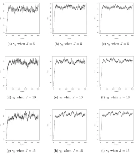
The misclassification rates of all models increase as shown in Table 2.6. The misclassi-fication rate of the unordered multinomial model is 10.75%, which is still good comparing to the result of Li and Yu (2008) who applied the functional segment discriminant anal-ysis on phoneme data having a misclassification rate of 18.5%. Figure 2.4 shows the cut-point γ2, γ3, and γ4 sampled by Metropolis-Hastings when J = 5,10,15, and they all converged in 500 iterations. Tables 2.7, 2.8, and 2.9 show the estimate and standard error of the posterior mean of the phoneme data under unordered multinomial probit model, multinomial logistic model, and ordered multinomial probit model, when J = 14,

(56)

(a)γ2 when J = 5 (b) γ3 whenJ = 5 (c) γ4 whenJ = 5

(d) γ2 whenJ = 10 (e) γ3 whenJ = 10 (f)γ4 when J = 10

(g)γ2 when J = 15 (h) γ3 whenJ = 15 (i) γ4 when J = 15

(57)

Table 2.7: Estimate and standard error of the posterior mean for the 5-class unordered multinomial model (J = 14)

estimate standard error

Θ                        

−7.80 54.08 −2.84 3.05 46.31 85.16 16.92 29.51 38.43 28.16 26.26 41.23

−14.55 −16.50 15.61 35.23

−25.56 −12.14 24.23 −13.36

−1.41 −3.17 −1.61 −23.32 21.99 −23.57 −21.25 −4.21

−11.41 2.50 −15.08 −14.98

−4.33 −4.78 −6.60 −5.70

−0.50 −13.51 −4.62 −6.74 4.66 −6.25 −6.19 −5.78

−10.02 −6.25 −13.68 −13.68

−21.88 −3.97 −16.29 −13.80

−23.61 −4.93 −7.44 −17.29                                                

1.05 1.05 1.05 1.03 0.87 0.83 0.81 0.88 0.66 0.66 0.74 0.72 0.97 1.00 1.16 1.19 0.96 0.93 0.92 0.90 1.00 1.04 1.08 1.134 0.98 1.11 1.10 1.13 0.95 1.14 1.02 0.98 0.96 0.99 1.08 1.09 0.85 0.98 0.74 0.80 0.70 0.73 0.94 0.92 0.81 0.86 1.09 1.06 0.74 0.69 0.94 0.99 1.02 1.10 1.14 1.11

(58)

Table 2.8: Estimate and standard error of the posterior mean for the 5-class multinomial logistic model (J = 14)

θ2

Estimate (1.81,10.18,3.24,−1.87,−9.06,2.82,14.20,−2.48,−4.15,−2.08,−1.85,−2.95,−4.14,−3.83) Standard error (0.18,0.57,0.49,0.22,0.33,0.20,0.66,0.12,0.31,0.13,0.33,0.45,0.58,0.48)

θ3

Estimate (4.01,25.83,8.13,0.84,−9.93,1.94,0.37,−4.14,−0.73,−2.80,−9.29,−2.49,0.27,2.19) Standard error (0.64,1.09,0.50,0.29,0.20,0.17,0.18,0.21,0.32,0.22,0.28,0.22,0.17,0.21)

θ4

Estimate (−8.04,6.63,−1.35,12.21,12.29,−2.26,−1.04,−0.18,−3.28,−6.06,−10.81,−5.54,−0.87,1.71) Standard error (0.35,0.27,0.16,0.44,0.73,0.34,0.19,0.30,0.29,0.28,0.65,0.24,0.22,0.16)

θ5

(59)

Table 2.9: Estimate and standard error of the posterior mean for the 5-class ordered multinomial model (J = 13)

γ2 γ3 γ4 θ

(60)

Chapter 3 Bayesian Change Point Detection

for Functional Data

3.1 Introduction

(61)

Rice, and S¨onmez (2018) proposed a method to uncover structural breaks in functional data that does not rely on dimension reduction techniques.

(62)

3.2 Model

We follow the formulation of Suarez and Ghosal (2016) for the structure of functional observations, who applied their model in the context of clustering. We extend their ap-proach to change point detection for functional data, which can be regarded as a special case of clustering with the constraint that for each characteristic, there are at most two clusters and they are linearly ordered. Suppose that the functional observations arise from true signals fi(t), t ∈ [0,1], i = 1, . . . , n, corrupted by some noise process, where

n denotes the sample size. We observe the functional data at some discrete time points. Then the model can be represented as

Yi(Tl) =fi(Tl) +εil, (3.1)

where εil is assumed to follow a normal distribution with mean 0 and variance σ2,

and is independent across i and l. Let Yi = (Yi(T1), . . . , Yi(Tm))T be the ith

ob-svervation at points T1, . . . , Tm, where Tl ∈ [0,1], for l = 1, . . . , m. Similarly, let

fi = (fi(T1), . . . , fi(Tm))T, and εi = (εi(T1), . . . , εi(Tm))T. For functional data, the

dis-crete wavelet transform (DWT) is one of the most common feature extraction technique. To implement the DWT,m needs to be a power of 2, and T1, . . . , Tm need to be

equidis-tant. For m that is not a power of 2, we can first smooth to obtain a function, and then take a power of 2 number of discrete points from that function. In terms of the orthonor-mal basis {φ0} ∪ {ψjk :j = 0, . . . , J −1, k = 0, . . . ,2j −1}, we can define the following

DWT operator (Antoniadis et al., 2013):

(63)

with βj = (βj,0, . . . , βj,2j₋₁). Applying the DWT operator onY_i =f_i+ε_i, then we have

W Yi =W fi+W εi, (3.3)

where W εi d

= εi by the orthogonality of W. Let α0 denote the scaling coefficient at the level 0, and βjk be the wavelet coefficients at the multiresolution level j, k. As a result,

(3.3) can be rewritten as

a₀(i) =α₀(i)+e(₀i), b_jk(i)=β_jk(i)+e(_jki), (3.4)

where e(₀i) and e_jk(i) follow a normal distribution with mean 0 and variance σ2_{, for} _k ₌ 0, . . . ,2j₋₁_{, j} _{= 0}_{, . . . , J}₋_1.

When the functional data are (essentially) observed continuously in time, we also consider the following infinite Gaussian white noise model

dYi(t) =fi(t)dt+σdBi(t), (3.5)

where Bi(·) are independent Brownian motions on [0,1]. Let

a(₀i)= Z 1

0

φ0(t)dYi(t), α

(i) 0 =

Z 1

0

φ0(t)fi(t)dt,

b(_jki)= Z 1

0

ψjk(t)dYi(t), β_jk(i) =

Z 1

0

ψjk(t)fi(t)dt,

e(₀i) =σ

Z 1

0

φ0(t)dBi(t), e

(i)

jk =σ

Z 1

0

ψjk(t)dBi(t).

(3.6)

(64)

To detect the change point of this sequence of functional data, we first find the change in each component, that is, we detect the change for each feature βjk, and we decide the

overall change point from them.

In the section on posterior consistency, we state the results only in terms of the infinite model. However, in practice, we can only work with the finite model. By letting β_jk(i) = 0 for all j > J, the infinite model can be related to the finite one with a random J. If the coefficients are obtained following the schema of Abramovich, Sapatinas, and Silverman (1998), then J will have a limiting Poisson distribution by Proposition 1 of Suarez and Ghosal (2016). Under this schema, the total number of nonzero coefficients also has a limiting Poisson distribution.

3.3 Prior Distributions

For each β_jk(i), we define the following probabilities:

P(β_jk(i)6= 0) =πj, P(β_jk(i)= 0) = 1−πj. (3.7)

As the wavelet coefficients of a signal function are sparse, Abramovich, Sapatinas, and Silverman (1998) proposed the following priors incorporating this characteristic feature of wavelet coefficients:

β_jk(i)ind∼ πjN(0, c2jσ

2_{) + (1}₋_π

j)δ0, (3.8)

where δ0 is a point mass at 0, and the hyperparameters in (3.8) are given by

(65)

and ν1, ν2, γ1 ≥0, and 0≤γ2 ≤1. A vague prior is placed onα0.

Let ψ be a mother wavelet function of regularity r. Consider constants s, p and q

such that max(0,1/p−1/2)< s < r, 1≤p, q ≤ ∞. If either

s+ 1 2−

γ2

p −

γ1

2 <0, (3.10)

or

s+ 1 2−

γ2

p −

γ1

2 = 0, and 0≤γ2 <1,1≤p <∞, q =∞, (3.11)

thenf ∈Bs

p,q almost surely, where Bp,qs denotes Besov space of index (p, q) and

smooth-ness s (Abramovich, Sapatinas, and Silverman, 1998). The prior on σ is given by

σ2 ∼IG(θ, λ), (3.12)

where IG stands for the inverse gamma distribution. Let g denote the density funciton of the inverse-gamma distribution.

3.4 Posterior Probabilities of Change Point

For anyj, k, letτjk denote the change point, and letτjk take possible values 1, . . . , n. Let

ρi denote the prior probability of changing at point i, where ρi > 0,

Pn

i=1ρi = 1, and

i= 1, . . . , n. Then the posterior probability of τjk =i is

P(τjk =i|b

(1)

jk, . . . , b

(n)

jk ) =

P(b(1)_jk, . . . , b(_jkn)|τjk =i)ρi

PN

l=1P(b (1)

jk, . . . , b

(n)

jk |τjk =l)ρl

(66)

The main problem is to compute the marginal likelihood P(b(1)_jk, . . . , b(_jkn)|τjk = i).

When τjk = 1, it is the initial state meaning no change. For τjk = 2, . . . , n, the marginal

likelihood is derived from four scenarios: change from zero to zero (which is no change), change from zero to non-zero, change from non-zero to zero, and change from non-zero to non-zero.

3.4.1 Initial State

When τjk = 1, this is the initial state. If the initial state is zero, then the marginal

likelihood is given by

(1−πj)

Z _n n Y

i=1

φ(b(_jki); 0, σ2) o

g(σ2;θ, λ)dσ. (3.14)

If the initial state is non-zero, then we have

πj

Z Z _n n Y

i=1

φ(b(_jki);ξ, σ2) o

φ(ξ; 0, c2_jσ2)g(σ2;θ, λ)dξdσ. (3.15)

Thus, the marginal likelihood of the initial state is

P(b(1)_jk, . . . , b(_jkn)|τjk = 1)

= (1−πj)(2π)−n/2

λθ

Γ(θ)

Γ(n/2 +θ) [

Pn

i=1(a (i) 0 )2

2 +λ]

(n/2+θ)

+πj(2π)−n/2

λθ

Γ(θ)(c 2

jn+ 1)

−1/2 Γ(n/2 +θ) hPn

i=1(a (i) 0 )2

2 −

c2

j

c2

jn+ 1

(Pn

i=1a (i) 0 )2

2 +λ

i(n/2+θ)

.

Bayesian Classification and Change Point Detection for Functional Data.

ABSTRACT

DEDICATION

BIOGRAPHY

ACKNOWLEDGEMENTS

TABLE OF CONTENTS

LIST OF TABLES

LIST OF FIGURES

Chapter 1

Introduction

Chapter 2

Bayesian Classification of Multiclass

Functional Data

2.1

Introduction

2.2

Model

2.2.1

Ordered Multinomial Probit Model

2.2.2

Unordered Multinomial Probit Model

2.2.3

Multinomial Logistic Model

2.3

Finite Random Series Prior

2.3.1

Ordered Multinomial Probit Model

2.3.2

Unordered Multinomial Probit Model

2.3.3

Multinomial Logistic Model

2.4

Marginal Likelihood and Model Averaging

2.4.1

Ordered Multinomial Probit Model

2.4.2

Unordered Multinomial Probit Model

2.4.3

Multinomial Logistic Model

2.5

Posterior Contraction Rate

2.5.1

Ordered Multinomial Probit Model

2.5.2

Unordered Multinomial Probit Model

2.5.3

Multinomial Logistic Model

2.6

Discriminant Analysis

2.6.1

Linear Discriminant Analysis

2.6.2

Quadratic Discriminant Analysis

2.7

Simulation

2.7.1

Data Generation

2.7.2

Basis Functions

2.7.3

Results

2.8

Application on Phoneme Data

2.8.1

Three Classes

2.8.2

Five Classes

Chapter 3

Bayesian Change Point Detection

for Functional Data

3.1

Introduction

3.2

Model

3.3

Prior Distributions

3.4

Posterior Probabilities of Change Point

3.4.1

Initial State