James Faber
Center for Communications and Signal Processing Electrical and Computer Engineering Department
North Carolina State University
ccsr-
TR-88/29FABER, L. JAMES
A
General Order Multichannel, Fast Least Squares Algorithm with Telecommunications Applications. (Under the direction of Sasan H. Ardalan and Sarah A. Rajala.)A new, general order, multichannel transversal fast recursive least squares al-gorithm is derived, using the principles of geometric projection. It is a generaliza-tion of prior multichannel fast LS algorithms, in that the orders of the several in-put channel joint process filters can be independently and arbitrarily specified. Like other fast LS algorithms, it has the property that update computations are of the same order as the total filter size, N. The algorithm is applied to a special two-channel case in which the unit-delayed joint process signal is taken as one of the input channels; this configuration is the equation-error form for LS pole-zero joint process estimation. A new and significant (2N operations per recursion) com-putational savings is derived for this configuration. Identification of an IIR bandpass filter is demonstrated for several conditions of over- and under-specification of filter orders. Several extensions to the algorithm are developed, in-cluding exponential memory, complex data, and normalized variables. The adap-tive algorithm is also applied to adapadap-tive equalization and echo cancellation, using a general purpose digital system simulator. The system parameters are chosen to
TABLE OF CONTENTS
...
...
Additional 0 bserva tions .
The Transmitter .
1 1 4 9 14 14 16 23 23 33 36 42 46 49 49 53 60 63 72 72 77 79 80 88 88 91 97 100 108 113
136
139 143Complex Data .
Predictors .
Filter Modeling Simulations .
Exponential Error Weighting .
ARMA System Identification .
Multichannel Output .
Least Squares .
Least Mean Squares .
5.1 6.2 6.3
6.4 The Normalized General Order Algorithm .
6. APPLICATION SIMULATIONS .
6.1 Introduction 6.2
6.3 The Channel .
6.4 The Receiver 6.5
7.
CONCLUSION
.
1.2 Linear Prediction and System Identification .
1.3 Outline of Dissertation .
9. APPENDIX: Simulation Modules and Topologies .
6.6 The Experiments .
6. ALGORITHM EXTENSIONS .
1.1 Adaptive Filtering .
8. REFERENCES .
2.1 2.2
3. THE GENERAL ORDER, MULTICHANNEL FTF .
3.1 Introduction
3.2 Generalized Updates of Operators .
3.3 Derivation of the Fast Multichannel Algorithm .
3.4 The Higher Order Multichannel Case .
3.A Appendix: Operators on Augmented Subspaces .
4. THE FAST ARMA PREDICTOR .
4.1 Introduction 4.2
4.3 4.4
2. ADAPTIV'E ALGORITHMS .
CHAPTER
1INTRODUCTION
Adaptive filtering is a fairly recent offshoot of the mature field of linear filter-ing theory [1], but has already proven to be extremely useful in many signal pro-cessing applications. In this chapter, a brief overview of adaptive filtering, and some of the major application areas is given. Via the concepts of linear prediction and system identification, a unifying categorization of these application areas is described. Finally, a general preview of the topics considered in the remainder of this work is presented.
1.1. Adaptive Filtering
pred-iction filters are based on prior knowledge of signal and noise spectral characteris-tics. Adaptive filters, however, can modify their parameters during operation to cope with unknown or changing conditions, and usually require little a priori signal
information.
Adaptive filtering has been applied to a wide range of signal processing appli-cations. Several representative examples are: speech analysis and encoding
[7]
[8], spectral estimation [9], antenna beam forming[10],
noise cancellation[11][12],
echo cancellation[13]-[15],
and voice- and data-channel equalization[16]-[19].
The application topics considered here will be primarily data-channel echo cancellation and equalization.A
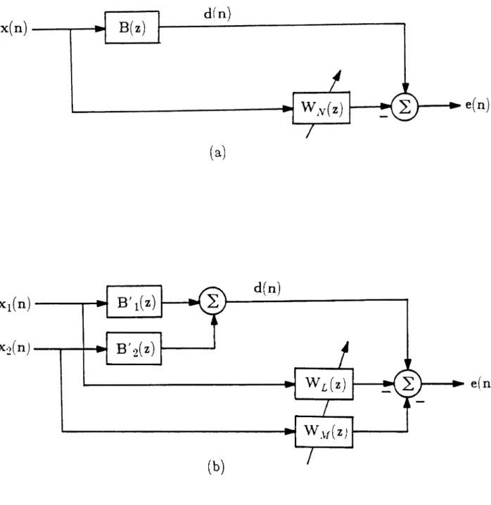
d(n)
x(n)
-...-.~Figure 1.1 Transversal F ilter
signal. An adaptive algorithm has the capability to modify the weighting coefficients, according to various rules, in order to produce a best prediction. These rules and a definition of "best" are discussed later.
The filter functions used here for sampled data signals are described mathematically by fixed-order linear difference equations with constant coefficients. That is, the relationship between an input sequence {x( n)} and an output sequence {d(n)} for a filter system can be written
L-l M
d (n)
=
L
biX (n -i)
+
L
aid (n - i) ,i=O i=1
and dynamically adjusted by various schemes, considered more fully in the next chapter.
1.2. Linear Prediction and System Identification
p(n)
+
u(n)
----r---~
~---.-..-.
u (n)
-1
z
Figure 1.2 Signal Separation
model [11][23].
System identification is used to estimate the coefficients of an assumed model for an unknown fixed (stationary) system, or to track the parameters of a system that is time-varying in an unknown way.
51
and LP are closely related since the prediction inherent in the latter requires (explicitly or not) the formulation of a linear signal-source model. However,51
normally requires access to the excitation signal] for the unknown process, as illustrated in Figure 1.3a. A useful equivalent system is shown in Figure 1.3b, which models both the system and51
filters with standard transversal forms, as in Figure 1.1. If the parameters of the identificationt Sometimes it is possible to create an estimate of the input signal, and achieve satisfactory results
I
,
x(n)
I
I I
I
ern)I
(a)
x(n) d(n)
e(n)
(b)
filters match those of the unknown system, the error signal will be zero. It is assumed that model orders are known or bounded. Figure 1.4a shows a special all-zero case of SI which is often used. The estimate of the unknown system out-put is created by filtering only the inout-put signal. Figure lAb extends this concept
to multiple input channels, which is one application of the algorithms developed in
this work.
Figure 1.5 shows another common configuration representing all-pole linear prediction. It is shown in [23] that LP can be considered a special case of system
identification. This assertion is supported by comparing Figure 1.5 to 1.3b. Here
only the system output signal is filtered; there is no access to the driving signal
x (n) in this configuration.
In this work, we will consider two primary application areas for these various
transversal filtering configurations: channel equalization and echo cancellation.
These are depicted in Figure 1.6, and have been drawn to match the general
sys-tem identification form, but with appropriate signal names. Equalization is
usu-ally considered an inverse filtering problem. However, with a simple linear
net-work transformation (see figures 1.6a and 1.3a), equalization can be considered a
system identification problem, where the unknown system to be identified, U(z),is
the inverse of the data transmission channel. This will be considered further in the
x(n)-~~
B(z)
dfn)
L.-_---..-....,~ W~v(
z)
(a)
...--~
e(n)
Xl(n)
B'l(Z)
---.-x~(n)-...--+--4_
B'
2(Z) ...----'
d(n)
t---~
e(n)
' - - - . . . W
J [ (Z) ~---'(b)
x(n )
---..i~A'(z)
Z-ld(n)
~~e(n)
Figure 1.5 All-Pole Linear Prediction
1.3. Outline of Dissertation
each of the input channel sub-filters. This required a conceptual modification of the derivation method. This development is shown in Chapter 3, and considers the configuration in Figure 1.4b.
In Chapter 4, the new algorithm is applied to a specific two-input configuration, known in system identification literature as the "equation error" for-mulation, as is illustrated in Figure 1.3b. This formulation allows a type of pole/zero (autoregressive, moving average, or ARMA) estimation of system param-eters. The general order capability was not previously known using the multichan-nel FTF algorithm in this application. A significant (2N+1)computational com-plexity reduction is then described and proven for this configuration, which previ-ously required O(12N) computations per update. This reduction was shown to be available with the other known fast recursive algorithms (FK and F AEST) as well, which had not been noted in earlier work.
Chapter 5 addresses several additional topics:
1) algorithm extension to include "exponential data memory". This mechanism for discounting older data is important in many practical applications, where the filter must continuously adapt to slowly changing conditions.
2) consideration of the multichannel output case, and the complex data case. These are shown to be related, and straightforward algorithm extensions.
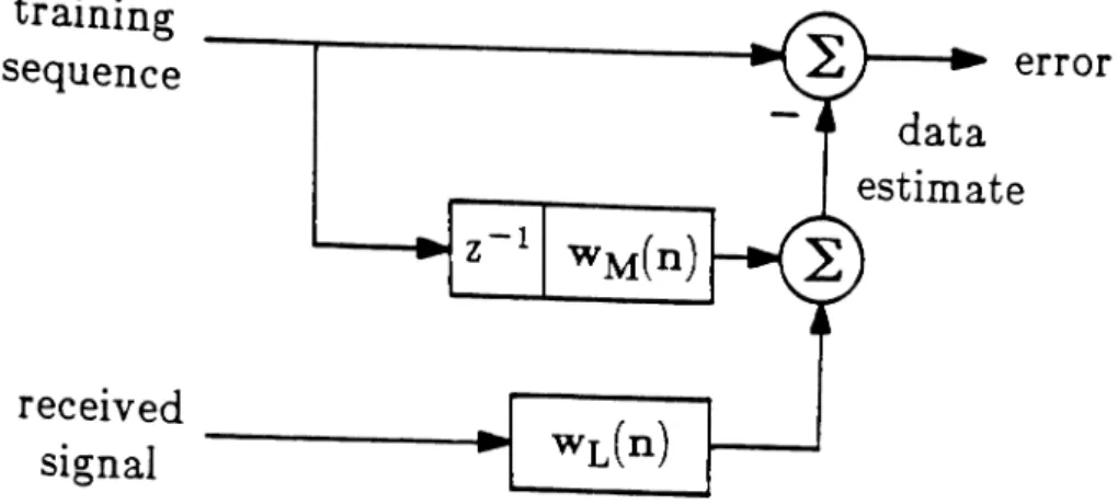
training
sequence
received
---...t
signal
error
data
estimate
from
far end
to
far end
Two-Channel Equalization
Echo
Path
Two-Channel Echo Cancellation
Figure 1.6 Transversal System Identification Applications
rx signal
algorithm variables. Such normalized forms have been shown to provide
superior numerical stability properties when compared to unnormalized ones;
this is particularly important in practical implementations with
limited-precision machines. However, the number of computations is increased, and it
is necessary to take square roots.
Chapter 6 summarizes several application simulations of the algorithm for the
Integrated Services Digital Network (ISDN) environment. This 192 kBps
data-transmission network specification is still under development; it is intended to
deliver a direct high-speed digital interface to subscribers on standard
uncondi-tioned 2-wire telephone lines [49][50]. This has created the need for adaptive line
equalization and adaptive transmit (near-end) echo cancellation. The capacity of
LS algorithms for rapid convergence make them attractive candidates for these
requirements. The flexible pole/ zero modeling capability can also produce
tremen-dous reduction of the model order (and consequently, computational burden)
required, compared to the current all-zero models. In a real-time situation, the
general order capability allows allotment of limited computational time to
particu-lar channels; it also provides independent specification of pole and zero orders in
the two-input equation error (ARMA) configuration described earlier.
The BLOSIM (Block Simulation) [51] system simulator program was used
to
build an end-to-end data transmission system, complete with adaptive equalizerCHAPTER
2ADAPTIVE ALGORITHMS
Adaptive filters require some mechanism to adjust their parameters so as to generate the "best" estimate of the joint process signal. Appropriate coefficients for the adaptive transversal form are normally computed by algorithms that attempt to minimize estimation error power, since this can be considered the meas-ure of a good estimate
[11].
Minimization of error methods in general can be divided into two classes, stochastic and exact. Stochastic methods attempts to minimize the statistical average (or mean) squared error signal. These methods assume short-term stationarity of the input signal, and are formulated in terms of the gradient of the error power, with respect to the filter parameters. The least mean squares (LMS) algorithm[11][21]
is a well known example of this class. Exact or least-squares (LS) algorithms exactly minimize the running sum of squared error values rather than the average error power.2.1. Least Mean Squares
(2.1)
where
cP
zz is the (NX N) autocorrelation matrix, and <Pzd is the (NX1) cross-correlation vector. Since the autocross-correlation matrix is Toeplitz (equal elements along major diagonals) and symmetric, direct inversion, O(N3 ) , is not required to implement (2.1). Instead, the order-recursive Levinson/Durbin algorithm [9], which is O(N2) , can be used. In practice, the true correlation statistics are usuallyunknown. They must be estimated from the incoming data, which requires
accu-mulation of several data samples before computations can be performed. Thus,
although theoretically optimal, this method performs poorly in practical parameter
estimation, particularly if the data record is short [9].
The best known time-recursive (sample-by-sample update) algorithm based
on statistical estimation is the LMS (least mean squares) algorithm. It is actually
iterative, rather than truly recursive, in the sense that it never achieves the
optimal Wiener solution mentioned above. It converges toward an assumed
optimal solution (based on stationary signal statistics) by using the instantaneous
error as an approximation of the gradient of the squared error function; small
adjustments are made to each weight value scaled by the data sample associated
with each weight. The LMS algorithm sequence is given as:
~ T
( a ) e ( n
I
n - 1)=
d(n) - d (nI
n - 1)=
d(n) - xN (n)wN (n - 1)(b)
wN(n)
=
wN(n-l)
+
)'xN(n)e(nln-l).
Here
XN(
n) defines the length N vector of input data at time n,XN(n)
=
[x(n), · · ., x(n-N+l)]Tand d (n In - 1) is an estimate of d (n), generated by the transversal filter of time
n -
1,
defined as the vectorwN(n-l)
=
[wo(n-l),· · ., wN_l(n-l)]TThe notation e (n
In -
1)means the prediction error at time n due to the prediction from the filter of time n -1. The small positive constant 'Y is chosen based upon input signal power and the filter size[11].
It can be observed that this algorithm requires --2N computations per update.It is known that the LMS gradient-estimate algorithm has convergence pro-perties that are related to the statistics of the input signal. In particular, conver-gence can be distinguished into converconver-gence modes, each related to a particular eigenvalue of the input signal. This is often undesirable since extremely slow filter convergence can result if there is large difference between the power in signal modes
[11].
In many applications, the LS algorithms described next have far supe-rior convergence properties [20][25][30][39]. Convergence of LS algorithms does not depend on signal statistics, but is determined by the filter size.2.2. Least Squares
e(n In)
=d(n) - X(n)WN(n)
wheree(nln)
=
[e(lln),
e(2In),···, e(nln)]T,d(n)
=
[d(l),
d(2), · · ., d(n)]Tare accumulations of scalar values defined earlier and
,
(2.3)
X(n)
=
z
[I]
x(2)
o
x(l)
o
o
x(n) x(n-l) . . x(n-N+l)
Thus, the sum of squared errors equals the error vector norm squared:
n
minimum ~
e
2(iln)=
rnineT(nln)e(nln). w.r.t,wN i=l(2.4)
Given the independence of the columns of X(n), a well known result of linear alge-bra is that for an overdetermined set of equations (here meaning more data sam-ples than adjustable weight parameters), a L8 solution for the filter parameters exists and is unique[46].
This solution can be found by vector differentiation, or by using orthogonality principles for linear systems of equations. Without showing details, the optimal length N filter for all data up to time n can be expressed in matrix form as:required. Recursive forms are often sought in these situations; such forms use the solution found at the previous data sample to help generate the solution including the new sample. This can provide a substantial economy in computations.
2.2.1. Recursive Least Squares. A fundamental observation is that the (NxN) data matrix product XTX grows in a systematic way. This matrix pro-duct, called the sample autocorrelation matrix, Rxx( n), is based on only a finite number of previous data samples, and is a statistical estimator of the true signal covariance matrix cDzz : Hence, a relationship to the stochastic approaches can be
seen. It is easy to show thatRxx(n ) can be decomposed as follows:
Rxx(n)
=
XT(n)A(n)X(n) = ~Rxx(n-l)+
xN(n)xJ(n) , (2.6)where A(n)
=
diag[A.n- 1, • • • , A., 1], and O<A.<l is now introduced as an exponential weighting factor. This factor is used for signals with non-stationary statistics in order to discount earlier data. Using this recursive form, the direct approach of
(2.4)
can be achieved in O(N3) computations, since matrix inversion isrequired.
( a ) e (n
I
n - 1)=
d (n) - wJ(
n - 1)xN (n )(b ) kN (n) = [~
+
xJ(
n )Q (n - 1)xN (n )r
1Q (n - 1)xN (n )(c) wN(n) = wN(n-l)
+
kN(n)e(nln-l)(d)
Q(n)=
~-l[Q(n-l) - kN(n)xJ(n)Q(n-l)](2.7)
The matrix
Q(
n)=
Rit(
n) is propagated directly in the algorithm, and thus no matrix inversion is required. The (NX1)vector kN isoften called the Kalman gain vector. Note the similarity of (2.7a,c) to the LM8 algorithm(2.2).
The Kalman gain vector is approximated there by )'XN(n), a scaled input vector.The RL8 algorithm makes recursive computation of the L8 filter solution pos-sible at each time increment. It requires O(N2) computations per update, where N
is the length of the transversal prediction filter. However, this is still infeasible for present real-time signal processors.
2.2.2. Fast RLS. A substantial reduction in RLS computational complexity was achieved with the Fast Kalman (FK) algorithm of Morph, Ljung and Falconer
[22] [25].
This algorithm made real-time L8 processing practical by requiring only-ION computations per update. This is very competitive with the relatively prim-itive LMS. The algorithm was derived by exploiting the shifted column property of the data matrix
X(
n).
The Kalman gain vector is computed via auxiliary for-ward and backfor-ward prediction filtersj for the input signal, which are also updatedrecursively.
This landmark was surpassed by two recently developed --7N recursive L8 algorithms, the fast transversal filter (FTF) [32] and the fast a posteriori error sequential technique (F AEST) [31]. These new filter algorithms were designed to update the transversal filter form and are recursive, i. e., the algorithms move to a new LS optimal solution from the old solution, as each new data point becomes available. Recent work by Wang [12] has shown the mathematical relationship between the FTF and F AEST algorithm solutions to the LS problem, each more efficient than the Fast Kalman algorithm. The single channel (scalar) FTF algo-rithm is shown in Table 2.1.
Table 2.1
The Single Channel (Scalar) FTF Algorithm
EQ
DIMOPS
ComputationI IXI N ef(nln-l)
=
x(n) - rR(n-l)xN(n-l)2 IXI 1 ef(nln)
=
-y(n-l)ef(nln-l)3 IXI I Ef(n)
=
Ef(n-I)+
ef(nln-l)ef(nln)4 IXI 2 )' + (n) = )' (n - 1)ef (n - 1)
e
i
1(n )5a NXI N+l f
[0
I [
1I
ef(nln-l)cN+1(n )= cN(n-l)
+
-fN(n-l) Ef{n-l)5b IXI 0 c+(n)
=
last element in cN+ 1(n) vector6 NXI N fN(n)
=
fN(n-l) + cN(n-l)et(nln)7 IXI 1 fb(nln-I)
=
Eb(n-l)c+(n)8 IXI 3 )'(n)
=
)'+(n)[l - J'+(n)eb(nln-I)c+(n)]-l9 IXI 1
.
eb{nln)=
),(n)eb{nln-l)10 Ix! I Eb(n)
=
Eb(n-l)+
eb(nln-l)eb(nln)[CN(n)] [bN(n-l)]
11 NXI N
a
=
CN+1(n)+
-1 c+(n)12 NXI N bN{n)
=
bN(n-l) + cN(n)eb(nln)13
lXl
N e(nI
n - 1) = d (n) - wJ(
n - 1)xN(n )14
lXl
1 e(nln) = ),(n)e(nln-l)15
Nxl N wN(n)=
wN(n-l) + cN(n}e(nln)7N
TotalOPS
"d= Pzd
2-D Subspace {Z}
Figure 2.1 Orthogonal Projection Onto a Subspace
CHAPTER
3THE GENERAL ORDER, MULTICHANNEL FTF:j:
3.1. Introduction
Fast transversal recursive least squares (RLS) algorithms
[311,[3
21 have filterupdate computational costs of order NI the filter length. Although these
algo-rithms suffer from long-term instability problems, their convergence superiority in many applications, compared to the common LMS (gradient) algorithms, have made them an active area of research. The purpose of this chapter is to present the derivation of a multichannel fast transversal recursive least squares algorithm with general order inputs. The approach in this derivation is to use the method of geometric projections onto a vector space defined by the input data. The applica-tion of this technique from linear algebra to the transversal filter case was first
given by Cioffi and Kailath [32]. The algorithm in this paper is distinguished from the multichannel algorithm shown there in which the order of the filter for each channel was constrained to be equal; here the order of each channel is completely arbitrary. This property, which allows greater flexibility in some applications, causes certain difficulties in the derivation. The key to resolving t.hesp difficulties is the use of permutation matrices, similar to those used by Falconer and Ljung
[22]
in their application of the fast Kalman algorithm to adaptive equalization. Thederivation in this chapter is a generalization of the work by Ardalan [33], which described an application to a particular two channel system in which the (unit delayed) output signal is used as one input channel. This is called the ARMA or pole/ zero estimation case, using the equation-error form for system identification [35]. The notation used herein is similar to that of [45].
3.1.1. Problem Description. The goal of the analysis is to recursively deter-mine the length N transversal filter W
N(
n), in the system shown in Figure 3.1,such that the optimal estimate of the (joint) process {d(n)} is formed by a transversal filtering of the two input processes {x (n)} and {y(n )}. These processes are real data sequences where data is assumed zero for n<0; this is called the
e(nln)
x(n)----l-d(
n) - - - .
y(
n)
- - - 1 - .(3.2)
prewindowed case. (Note: only two input channels are considered for notational simplicity; the extension to the arbitrary p-channel case will be considered in sec-tion 3.4.) Here optimality is defined in a cumulative or exact least squares sense; this can be explained as follows. The estimation error incurred at time i, based upon the filter at time n is defined
e(iln)
=
d(i) - d(iln)
=
d(i) - wR(n)zN(i),
l~i<n,
(3.1)where
d
(i
In) represents an estimate of d(i) using the transversal filter of time n, and zN(i) is a length N vector of past input samples from both channels:(NX1) zN(i)
=
[xl(i), yZ(i)]T, with N = L+
M, (LX!) xL(i)=
[x(i), x(i-l), , x(i-L+l)]T, and(Mxl) YM(i)
=
[y(i), y(i-l),
, y(i-M+l)]T.
The length N transversal filter W
N(
n) is partitioned into subfilters of lengths Land M, corresponding to the respective input channels. Thus it is desired to find the
n
minimum ~ e2(i In).
w.r.t. wN(n) i=1
(3.3)
This is the well known least squares (L8) problem, which can be succinctly
expressed in vector notation.
latest time:
(nXl)
x(n)=[x(l),
x(2),"', x(n)]T, y(n)=[y(l),
y(2),"', y(n)]T (3.4)A similar vector is defined with samples of the joint process {d(n )}. It is also con-venient to define a 'pinning vector'
[41][42][32]
(nxl)
1T(n)=[O,···,O,l]T.
(3.5)
This is the unit vector in the direction of the newest data sample, and will prove useful later.
A vector
z(
n) is now defined with columns comprised of the input vectors. Additionally, Zb(n) is defined with columns of input vectors that are each time delayed by the order of the filter assigned to that channel:(nX
2)
z(
n)=
[x(
n), y(n) ] ,(3.6)
Here z-L for example, is the L-unit time delay operator. Note that the vector
Zb(n) is still of length n, but with leading elements of zero since the data is prewin-dowed. It is also convenient to define the final rows of these vectors as
(2Xl)
z(n) = [x(n), y(n)]T =zT(n)7r(n),
zb(n) = [x(n-L), y(n-M)]T .(3.7)Note that these rows can be generated by inner products with
1T(
n). If an (nXN)(3.8)
o
y(1)
y(n-M+l) x(l)
x(n) x(n-l)
=
Zo(
n) =[Xo(
n),Yo(
n ) ]=
[x(n), z-lx(n), · · · , Z--L+lx(n), y(n), · · · , Z-M+ly(n)]x(l) 0 0
I
y(l) 0x(2) x(l)
I
y(2) y(l)I
I
x(n-L+l)
I
y(n) y(n-l)then a vector representing the estimation error resulting from the transversal filter W N (n) can be defined
(n x
I]
e(nln) = d(n) - d(nln) = d(n) - ZO(n)wN(n), (3.9)where each element in e(nln) corresponds to a scalar error from (3.1). A row of
Zo(
n) would represent the data in the transversal filter WN(
n) at a particular time; row i ofZo(
n) is then zJ( i) defined in (3.2).Other useful matrices can be defined. If each column of
Zo(
n )is unit delayed:(nXN) Zl(n)
=
[X1(n), Y1(n)]=
[z-IXo(n), z-lYo(n)]= [z-lx(n), · · ., z-Lx(n), z-ly(n),· .. , z-My(n)]. (3.10)
Consider the
Zo(
n)
matrix augmented with one additional column for each of the input channels, representing the addition of a tap for each channel subfilter:(nXN+2) Z+(n)
=
[Xo(n), z-Lx(n), Yo(n), z-My(n)]=
[x(n), Xt(n),y(n), Yt(n)]
(3.11)Note that this augmented matrix can be described in two ways, using the previ-ously defined matrices. The final row of Z+(n) defines a vector, which can also be
(N+2Xl) zN+2(n)
=
[xl(n), x(n-L), yZ(n), y(n-M)JT=
[x(n),xl(n-l),
y(n),yZ(n-l)JT.
(3.12)3.1.3. Projection Operators. From (3.9), each element (tap) of W
N(
n) definesa weight applied to a particular column of Zo( n); i.e., the estimate vector
cl(
nIn) is a linear combination of the columns. Equivalently, the estimate vector must lie in the column space of Zo(n). The columns span a subspace of Rn , the space of all real-valued, length n vectors. These key observations lead to the concept of projection onto a subspace as a means of locating the least squares error estimate of a vector within that subspace[43].
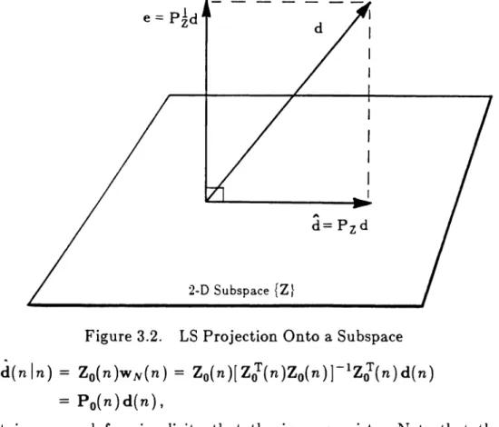
It is a well known result of linear algebra that the minimum length (norm) error vector corresponds to that estimate of a vector found by taking its geometric (perpendicular) projection onto the subspace of input vectors. This is shown conceptually in Figure 3.2 for a two-dimensional subspace. Note that the error vector e(nIn) and the estimate vectorcl(
n In) are perpendicular; this is a general orthogonality principle for LSsolutions. An opera-tor matrix P can be formed having the desired property of projection onto a par-ticular subspace. The operator which projects onto Zo(n) is found by solving the matrix equation:min eT (n
I
n)e(nIn) = min e(n ) .w.r.t.W N(n) w.r.t.WN(n) (3.13)
Differentiating e(
n)
with respect to WN(
n)
and equating to zero yields theLS
"
d= Pzd
2-D Subspace {Z~
Figure 3.2. LS Projection Onto a Subspace
d{nln)
=
ZO{n)wN{n)=
Zo{n)[Zl{n)Zo{n)r1Zl{n)d{n)= p
o(
n) d( n) , (3.14)where it is assumed for simplicity that the inverse exists. Note that the least squares estimate of an arbitrary vector is obtained by premultiplying by a matrix that is a function of only the input data vectors! The projection operator onto the subspace of
Zo(
n) is thus defined(nxn) Po(n) = Zo(n)[Zl(n)Zo(n)r1Zl(n).
The operatorPI
(n)
is similarly defined for the Zl(n)
subspace.(3.15)
An operator can also be found to generate the LS error vector which is
orthog-onal to the
Zo(
n)
subspace. Substituting (3.14) into (3.9) givese(nln)
= d(n) - Po(n)d(n)=
[I -
Po(n)]d(n)=
P!(n)d(n). (3.16)(3.17)
(nXn )
P~(
n) = I - Po(
n ) ; similarly,(nX n)
P1(
n)=
I -P
l(n) ·These operators generate the projection of a vector perpendicular to their defining
subspaces.
3.1.4. Tranevereal Filter Operators. From (3.14), the optimal transversal filter can be written
WN(n) = [Zl(n)Zo(n)]-lZl(n)d(n).
A transversal filter operator (matrix) can then be defined
(3.18)
(3.19) By premultiplication, this operator creates the transversal filter (for the input data) which would generate the unique L8 estimate of a vector on the subspace of
Zo{
n). Similar operators can be defined on the other subspaces shown earlier:(NXn) K1(n ) = [Z!(n)Zl(n)]-lZ!(n),
(N+2Xn) K+(n) = [ZJ(n)Z+(n)]-lZJ(n). (3.20a,b)
Several transversal filters can be generated using these operators on previously defined vectors, including a forward predictor for the input channels, a backward predictor, and a gain filter. These filters, and their associated prediction errors and residuals (squared error vector norms) are summarized with definitions in Table 3.1. The need for these quantities will be seen during the algorithm deriva-tion. Most are not directly evaluated from their definitions; instead, relationships between the quantities are exploited to allow tremendous savings in computations.
Table 3.1
Definitions for the General Order, Two-Channel FTF Algorithm
EQ
I
DIM
II
DEFINITIONTransversal Filters
1 NXI WN( n )
=
Ko{n )d( n )
joint predictor 2 NX2 fN(n)=
K1
(n )z(n )
forward predictor3
NX2 bN{n)=
KO{n)zb(n) backward predictor 4 NXI gN(n)=
Ko(n )1T(n )
gain (unit predictor)5 NXl cN{n)
=
)'-l(n)gN(n) normalized gain6 N+2xl gN+2(n)
=
K+{n)7T(n) augmented gain 7 N+2xl cN+2(n)=
)'.;1(n)gN+2(n) norm. augm. qain.8 N+2xl
gk+2(n)
=
K!(n)1T(n)
[oruiard shilted augm. gain 9 N+2x! ct+2(n)=
'Y.;1(n)gk+2(n) norm. f. shift. augm. gain 10 N+2x!gt +2{ n )
=
Ki (
n)7T( n )
backward shift. augm. gain 11 N+2xl ct+2(n)=
'Y.;1(n)gt+2(n)
norm. b. shift. augm. gainPrediction Errors
12
lXl
e(nln-l)=
d(n)-wJ{n-l)zN(n)13
IX!
e(n/n)=
d(n) - wZ(n)zN(n)=
<d(n),P~(n)1T(n»
14
2xl
ef(nln-1)=
z(n) - rZ(n-1)zN(n-1)15
2Xl
ef(nln)= z(n)-rZ(n)zN(n-1)=<z(n),P1(n)1T(n»
16
2Xl
eb(nln-l)=
zb{n) -bJ{n-l)zN{n)
17
2xl eb(nIn) =
zb(n) - hZ(n)zN(n)=
<zb(n),P~(n)1T(n»
18
IXl
-y(n)=
1-gZ(n)zN(n)=
<1T(n),P~(n)1T(n»
19
lXl
'Y+(n)=
1- gJ+2(n)zN+2(n) Residuals20 !x!
e(n) = <e(nln),e(nln»
=
<d(n),P~(n)d(n»
21
2X2
ef(n)= <ef(nln),ef(nln»= <z(n),P1(n)z(n»
the pinning vector 7T(n). The associated prediction error
'Y(
n) (see Table 3.1.18) was shown in[41]
to be the squared cosine of the angle betweenz(
n) and its esti-mate in the subspace of Zl(n). Thus,'Y(
n) is a measure of the amount of new in-formation (innovation) in the latest data sample, and is a key parameter in the derivation.3.1.5. Permutation Oper-at.ora. The permutation operators S defined here are
row-permuted identity matrices, such that pre-multiplication of a vector by Swill cause rearrangement of the vector's rows. Such matrices have the important pro-perty of orthogonality: SST = I or ST
=
8-1. The (N+2)x{N+2) 'forward' and'backward' permutation operator matrices, SI and Sb respectively, are defined by their effect on the augmented vector zN+2{n):
(3.21a,b)
From these definitions it is easy to also describe matrix column rearrangement:
Z+(n)SJ
=
[x(n), y(n), X1(n), Y1(n)]=
[z(n), Zl(n)],Z+(n)Sl = [Xo(n), Yo(n), z-Lx(n), z-My(n)] = [Zo{n), zb(n)]. (3.22a,b)
that augmenting columns naturally appear 'inside' the data matrix. Thus, perrnu-tation operators are used to first rearrange these columns so that the update forms may be properly applied.
Using the property of orthogonality of the permutation operators, the transversal filter operator for the permuted, augmented subspace can be deduced:
(N+2Xn) K{{n)
=
[SfZ;(n)Z+(n)SJr1SfZ;(n)=
SfK+(n),(N+2Xn) Ki(n)
=
SbK+(n). (3.23a,b)Pre-multiplying a vector with a transversal filter operator K yields the transversal filter which would generate the LS error estimate of that vector, in the defining subspace of the operator. Each row of K transforms the vector into a particular filter tap. Thus, permutation of the rows of K is equivalent to permutation of the elements of the transversal filter. This concept is seen in the following equations for permuted gain filters (refer to Table 3.1):
(N+2Xl) gt+2(n)
=
Sf gN+2(n)=
SfK+{n)7T(n)=
K{(n)7T(n),(N+2xl) gt+2(n)
=
SbgN+2(n) = Kt(n)1T(n).Using the orthogonality property of S, these can be combined to show:
3.2. Generalized Updates of Operators
(3.24a,b)
3.2.1. Projection Operator Order Update. In order to derive the recursive algorithm, it is necessary to consider the problem of updating the projection opera-tor when new columns are added to the defining subspace. In general, the projec-tion operator onto a subspace X is defined
P
x
=
X <X,X> -lXT=
X(XTX)-lXT (3.26)where
< ·,·
>
represents the inner product on the subspace X. The properties of symmetry (P*=
Px ) and idempotence (P$c=
Px ) are readily verified for this operator. The general perpendicular projection operator can be defined:(3.27)
(3.28) also with the properties of symmetry and idempotence. Augmenting the subspace X with columns Y yields the following order updates for the projection operators:
PX,y
=
Px
+
p{P~y}
=
Px
+
p-ky«v,
p~y> -lyTp~,
P~,y
=
I - PX,Y=
P~
-P~<y, p~y> -lyTp~.
The projection operator is updated by incorporating only the new information from the augmented columns, namely that portion of the subspace spanned by the new columns which is orthogonal to the old subspace. Pre- and post-multiplying (3.28) by arbitrary vectors uT and v gives the useful identity
(3.29)
3.2.2. Transversal Filter Operator Order Update. The general transversal filter operator defined on the subspace X is
KX
=
<XX>-lX
, T ,and the following properties are easily demonstrated:
KxX
=
I,
XK
x
=
P
x .
K P
x x
=
K
x-From (3.31) and assuming XnXN, YnXp
[
IN ONXP]
Kx,y[Xn x N , Yn x p ]
=
IN+p=
0 I ·pXN p
Thus, using
(3.28),
the update for post-appended columns is(3.31 )
Kx,y
=
Kx,YPX,Y
=
[~x]
+
[-~xY]<Y, p~y>-lyTp~.
(3.32a) Similarly, it can be shown for prepended columns(3.32b)
3.2.3. Time Updates of Operators. Using (3.28) and (3.32a) with X=Zo(n) or
X=Zl(n)
andY=1T(n),
it can be shown thatand
and
[
p~(n
-1) 0]
pl
0,11'(n)=
OT 0[
P1(n - 1)
0] .
pl
(n)=
1,11' OT 0
(3.33)
Also, the transversal filter operator for the subspace augmented with
1T(
n) can be expressedKo(n
-1) 0K
O'1r(n)=
-zJ(n)K
o(n-1)
1
K
t ( n - l )0
K
1,1r(n)=
-zR(n-1)K
1(n-1)
1 · (3.34)
vector space derivation of the fast transversal algorithm.
3.3. Derivation of the Fast Multichannel Algorithm
Now that the preliminary updates and definitions have been determined, it is possible to derive a recursive solution to the L8 problem posed initially. The derivation basically requires substitutions into the update forms, and reductions using the definitions. The derivation begins with an update form for the joint prediction filter, and then systematically finds recursions for other variables as they appear. The use of the permutation operator is seen in sections 3.3.3, 10, 11, which deal with updates of the gain filter and its associated prediction error. The complete algorithm is summarized in Table 3.2 in proper order of execution. An operation count is also provided for each recursion.
3.3.1. Joint Prediction Filter. From (3.32a) with X
=
Zo(
n), Y=
1T(
n),K
O,1T(n)=
[K~n)]
+
[-K
o(;)7T(n)]
<7T(n), PMn)7T(n»
- l7TT(n )P-b(n )
(3.35)Post-multiply (3.35) by d(n), and use expansion (3.34) with definitions (3.1.4, 18):
[
K o(n - l )
xx01
1[d(n-l)]
d (n ) =[Ko(n)]
0 d(n ) -[gN(n)]
_ 1 'Y - l(n )<
1T(n), Pt(n)d(n )>
Take just the upper partitions and use (3.1.1, 5, 13)Table 3.2
The General Order, Two-Channel Transversal RLS Algorithm
EQ
DllvI OPS Computation1 2XI 2N e/(nln-l)
=
z(n) - f~{n-l)zN(n-l) 2 2XI 2 e/(nIn)=
-y(n-l)ef(nIn-I)3a 2x2 3* Ef{n)
=
€f{n-l) + ef{nln-l)efT(nln) 3b 2x2 5* €f-l( n): 2 X2 matrix inverse4 IXI 6 " + (n)
= )'(
n - 1) - efT(nIn)€i
1(n )e/ (nIn)5a N+2xl 2N+2 cN+2(n)-, - [ 0
I [
121 -
1I
-
1cN(n-l)
+
-fN(n-l) *=-, (n)e,(nnh+
(n)5b N+2Xl 0** ct+2(n)
=
SbSJC~+2{n)5c 2Xl 0** c~(n)
=
last 2 elements in Ct+2(n) vector6 Nx2 2N fN(n)
=
fN(n-l)+
cN{n-l)efT(nln)7 2xl 4 eb(nln-l)
=
€b(n-l)c~(n)8 lxl 4 ,,( n)
= )'
+(n )[I - )'+(n )ebT(n In - I )c~(n ) ]- 19 2xl 2 eb(nln)
=
,,(n)eb(nln-l)10 2x2 3* Eb(n)
=
Eb(n - 1) + eb(nIn - 1)ebT(n In)[CN(n)
I
[-bN(n-l)]
11
s
«:
2No
=
Ct
+
2(n) -+1
2 c~(n ) 12 Nx2 2N bN(n)
=
bN(n-l) + cN(n)ebT(nln)13
lxl N e(nln-l)=
d(n) - w~(n-l)zN(n) 14 lxl 1 e (nIn)= ,,(
n )e(n In -1)15
Nxl N wN{n)=
wN(n-l) + cN{n)e{nln)12N
*
matrix symmetry allows reduction in OPS.TotalOPS
+32
**
since vector rearrangement is predetermined.3.3.2. Joint Process Error. Transpose (3.36), post-multiply by
ZN(
n)
and sub-tract from d(n):d(n) - wJ(n)zN(n)
=
d(n) - wJ(n-l)zN(n) - e(nln)zJ(n)zN(n)
(3.37)With definitions (3.1.12, 13)
e(nln)
= ~(n)e(nln-l). (3.38)3.3.3. Gain Filter. From (3.22), with Y=
z(n)
and X=Zl(n),
the subspace[Y,X] is
Z+(n)Sl;
the associated TF operator isK!(n).
Use (3.32b) andpost-multiply by 71"(n ),
K!(n)11"(n)
=
[Kl~
n)]11"(n)+ [_
K
1
(
~
)z(n) ]<
z(n), P1(n)z(n ] -1<
z(n), P1(n)11"(n»It is readily shown that K
1(
n)1T(
n) =gN(
n-1); with definitions (3.1.2, 8, 15, 21)gk+2(n)
=[gN(~-l)]
+
[_r:
2
(n ) ]Ej l(n )e/ (n ln ) .
(3.39)Similarly, from (3.32a) with X=
Zo(n),
Y= zb(n),post-multiply by1T{n)
· <
zb(n
),Pt(
n
)zb(n)
>
-1<
zb(n
),Pt(
n
)71" (n)
>
From definitions (3.1.3, 4,10,17,22)
gt+2(n)
=
[gN~n)l
+
[-b~(n)lEb-l(n)eb(n'n)
or with (3.25)
[
gN{n ) ]
o
=
Sb
SJ
gt
+2 (n)
+
[bN(n)]
_
1 2E
b-
1(n )eb(n
In) ·From (3.40)we define the last (2x 1)element of gt+2{n) as
g~(n) =
Eb-1(n)eb(nln).
Also, with
(s.i.m,
the last element ofct+2{n) is defined(3.41)
(3.42a)
(3.42b)
3.3.4. Forward Prediction Filter. Use (3.32a) with X
=
Zl(n), Y=
1T(n)and expansion (3.34);post-multiply by z(n) and take only the top partition:
(3.43)
3.3.5. Forward Prediction Error. Transpose (3.43), post-multiply by
zN(n-l),
and subtract fromz{n):
z{n) - fR{n)zN(n-I)
=
z(n) -
rJ'(n-l)zN(n-l) - e/(nln)cJ'(n-l)zN(n-l) With definitions(3.44)
(3.45)
3.3.6. Forward Prediction Residual. Use (3.29) with X
=
Zl
(n), Y =n(
n),and
u
=
v=
z(
n),<
z(n),
Pt,1T(n
)z(n )
>
=
<
z(n ),
Pt(n
)z(n )
> -
<
z(n),
Pt(n
)1T( n )> ·
· <1T(n),
Pt(n)1T(n»
-l<1T(n), P{(n)z(n»
[
Z(
n-1)]
Use (3.33) and partition z(
n)
=
zT( n)
,
(3.47)
3.3.7. Backward Prediction Filter. Use (3.32b) with Y=1T(n), X=Zo(n),
postmultiply by Zb(n).
(3.48)
3.3.8. Backward Prediction Error. Transpose (3.48), post-multiply by ZN(n)
and subtract from Zb(n):
zb(n) - bJ(n)zN(n)
=
zb(n) - bJ(n-l)zN(n) - eb(nln)cJ(n)zN(n)
(3.49)
With definitions(3.50)
3.3.9. Backward Prediction Residual. Use (3.29), with X
=
Zo(
n),Y =
7T(n),
and u = v = zb(n); use (3.33) and partition zb(n) =(3.51)
3.3.10. Gain Error. Use (3.1.19) and substitute (3.24a)
I'+(n)
=
1 -gkr2(n)S,zN+2(n).
Use (3.39) and (3.21a). Definitions (3.1.15, 18) provide
I'+(n)
=I'(n-l) - el(nln)ejl(n)e,(nln).
Similarly, use (3.1.19) and substitute (3.24b),l'+(n)
=
1 - g~\2(n)SbzN+2(n) Now, use (3.40) and (3.21b).)' + (
n)
= )' (n) - ebT(n
In)Eb-
1(n ) e
b (n In) .
Thus, with (3.42b) and (3.50), (3.53) becomes
(3.53)
(3.54)
3.3.11. Normalized Gain Filter. Substitute (3.43) into (3.39); use (3.53) and divide through by )'+ (n )
Ck+2(n)
=
[CN(~-l)]
+
[_fN~:_l)]Eil(n)ef(nlnh;l(n).
Similarly, use (3.40), substitute (3.48), and divide by'Y+(n)
(3.55 )
(3.56)
3.3.12. Simpler Backward Prediction Error Update. Instead of using the definition (3.16) to evaluate
eb{n
In
-1), requiring2N
multiplies,a
simpler form can be found. Post-multiply (3.51) by (3.42b) to yieldEb{n)c~(n)=
)';l{n)eb{nln)
=
eb(n-1)c~(n)+
eb(nln)ebT(nln-1)c~(n).Using simple algebra,
(3.57)
Edn-l)c~(n)
=
,,;l(n)ednln)[l - ,,+(n)e?(nln-l)c~(n)], (3.58)but from (3.54), the term in brackets is equal t.o )'+(n)'Y
-l(
n). With (3.50),eb(nln-l) = Eb(n-l)c~(n). (3.59)
3.4. The Higher Order Multichannel Case
This section considers some extensions of the previous sections to the general p-channel case, rather than only two input channels. In general, this is a straight-forward procedure and will not be shown here in detail, since only a change in the dimensionality of vectors and matrices used in Table 3.2. is required. However, from a computational standpoint, certain savings are possible, and derivations of these will be shown next.
If the number of channels p becomes large, table equation (3.2.3b) becomes computationally costly, since a pXP matrix inverse is required. With standard Gaussian inversion, this will require 0 (p3)multiplications. It is possible to reduce this to an 0
(p2)
process, as will now be described.From (3.47) we can write
ef ( n
I
n - 1) el (
nIn)
=
€f (n ) - €f (n - 1)=
A (3.60)where matrix A is a notational convenience. Now taking (3.52), and premultiply-ing by ef (n
In
-1) and post-multiplying by el (
nIn)
gives~+(n)A
=
~(n-1)A - ~(n-l)AejI(n)AFinally, post-multiplying by A-Ief(n), and re-arranging gives
(3.61)
€f(n)
=
'Y+
1( n )-y( n - 1)€f (n - 1) (3.62)(3.63a,b)
(p
xi)
a(n)=
Ei
1(n - 1)ef (nIn - 1)(1xi) a ( n) = [1
+
el (
nI
n)a(n )r
1The algorithm can be manipulated so that these variables will recur and thus reduce required computations. Note that a(n) requires p2multiplications (OPS) to compute and a(n) requires p
+
lOPS. Substituting (3.62) for Ef (n) in (3.52) andre-arranging gives
)'+(n)
=
),(n-l)a(n)Using the matrix inverse lemma with (3.47), we can then write
(3.64)
ejl{n)
= ei1 ( n - l ) - 1'+(n)a(n)aT{n) (3.65) Because of the symmetry of the Ef matrix, this equation requires p+
lh(p2+
p)OPS to compute. (It is interesting to note that (3.62) can not be used directly to update e
i
1(
n). The scalar multiplication would erroneously preserve the initial value of the matrix.) Finally, with the new relationships, (3.55) becomesct+p(n) =
[CN(~-l)l
+
[-fN~:-l)la(n)
This equation requires pN OPS to implement.
(3.66)
Table 3.3
The General Order, p-Channel Transversal RLS Algorithm
EQ DIM
OPS
Computation1 pXl pN ef{nln-I) = z(n) - f~{n-l)zN(n-1)
2 px1 p ef(n In) = 'Y( n -1)ef (n In - 1) 3a pxI p2 a( n) = Ef-1(n - I )eI (n In - I )
3b lxl p+l 'Y+(n) = 'Y( n - I) [ I + eIT(n In) a( n )]-1 4 pxp 'h(p2+3p) E /- 1(n) = E
i
1(n - 1) - 'Y+ (n )a( n )aT (n )5a N+pxl pN
c~+p(n)=[CN(~-1)]+[-fN~:-l)]a(n)
5b N+pXl 0 ct+p(n) = SbSJc~+p(n)
5c pxt 0 c~{n) = last p elementsinct+p(n) vector
6 NXp pN fN(n) = fN(n-l) + cN(n-l)e/T(nln) 7 p
x
I p2 eb(nln-l) = Eb(n-I)c~(n)8 lXl p+2 'Y(n)
=
'Y+(n ) [1 - 'Y+(n )ebT(nI
n - 1)c~(n ) ]-19 pxi p eb(nln)
=
'Y(n)eb(nln-l)10 pxp lh(p2+p) Eb(n) = Eb(n-I) + eb{nln-l)ebT(nln)
[cN(n)]
[-bN(n-l)]
11 NXI pN
o
p =c
t
+P (n) - Ip C~(n )
12 NXp pN bN(n)
=
bN(n-1) + cN(n)ebT{nIn) 13 Ixl N e(nln-I)=
d(n) - w~(n-l)zN(n) 14 IXI 1 e (n In)=
'Y{ n )e (n In -1)15 NXI N wN(n)
=
wN(n-l)+
cN(n)e(nln)APPENDIX3A
Operator
Expansions for 1T-Augmented Subspaces
This appendix shows detailed proofs of equations (3.33, 34), decompositions of the projection and transversal filter operators for a subspace augmented with the
npinning" vector, 1T. These are important relationships, used in the derivation of
all the transversal filter update equations. They are also critical in the proper development of the exponentially windowed version of the FTF algorithm, as described in Chapter 5.
Theorem 1: Given an (nX N) matrix U with its final row partitioned:
U =
[~l
(3A.I)
Define an augmented matrix V with the (n
x
i) unit vector 1T right appended:v
=
[U 1T]
=
[~ ~
1
(3A.2)
If the transversal filter operator for an arbitrary subspace X is defined
K
x
=(XTX)-l
x"
(3A.3)
then the transversal filter operator for the subspace V can be expanded as
K
v
=
(3A.4)Proof: Substituting
(3A.2)
into the definition of Kv givesFrom a matrix inversion lemma for partitioned matrices
[46],
ifp-l is defined, q, r are column vectors, and s is scalar, then[
p
q]-l
=[p-1+tP~1~:P-1
-tP
t
- 1
q]
(3A.6)rT s -tr P
with
t
=
[s -
rTp-lq]-1. This expansion can be verified by direct multiplication.For convenience, now define
B = ATA
+
aaTThis then gives
(3A.7)
_
[(B-1+~B-1aaTB-1)AT
(B- 1 +~B-1aaTB-1)a
-~B-1a]
K v - -QaTB-1AT TB-1 (3A.8a,b)
tJ -~a a
+
~r3
=
[1 - aTB - 1a ]- 1From a lemma for the inverse of summed matrices [46], if p-l is defined, q, rare column vectors, and s is scalar, then
[P + qsrT)- 1
=
p-l_ tp-lqrTp-l with t=
[8 -
rTp-lq]-l. Thus, (3A.7) provides(3A.9)
a-I
= (ATA)-l - c:x(ATA)-laaT(ATA)-l (3A.I0a,b) ex=
[1+
aT(ATA)-la]-1It can readily be shown that ~ = ex-1. These definitions can now be substituted
into each term of (3A.8a) to complete the proof. For an alternative proof, evaluate equation (3.32b) with U =
1T'.o
This implies that the estimate vector is a linear combination of the columns of the subspace. The transversal filter operator, in effect, determines the particular weight to apply to each column to generate the estimate vector. The first row of the transversal filter operator matrix (times the arbitrary vector) generates the weight for the first column, etc. Consider now the right augmentation of the sub-space by the 1T vector. This new column is also weighted to contribute to the LS estimate vector; however, since it is only non-zero in the last row, its column weight cannot affect the estimate error except in the final row. Thus, since squared error is minimized for the LS estimate, the weight for the 1T column is selected to exactly zero any estimation error due to the last row. The LS weights for the other columns are determined as if the final row did not exist. This is exactly what (3A.4) expresses. The name "time annihilation" vector sometimes given to 1T is
thus explained, since the final row of the subspace matrix contains the most recent data values.
Theorem 2: If U and V are defined as in theorem 1, and the projection operator for the subspace X is defined
Px
=
X(XTX)-lX
Tthen the projection operator for the subspace V can be expanded as
(3A.l1)
(3A.12) P
v
=
[:~ ~
1
Proof: From the operator definitions (3A.3, 11), Py
=
VKy . Substitute (3A.2)Finally, there is an additional simple theorem that will prove useful in later derivation.
Theorem 3: Given A = ~B, with A, B matrices and ~ scalar; then
PA
=
PBK
A=
r3-
1K
BProof: Direct substitution into the operator definitions {3A.3, 11).0
CHAPTER
4
THE FAST ARMA PREDICTOR:I:
4.1. Introduction
The application of transversal least squares (LS) algorithms to certain prob-lems of real-time system identification has become feasible with the discovery of "fastn recursive LS algorithms. These adaptive algorithms are known as the Fast Kalman
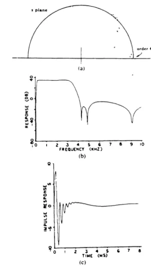
[22),
F AEST[31),
and the FTF[32)
algorithms. Because the algorithms can perform their update computations in a time directly proportional to the filter length, N, they are suitable for real-time implementation. Since these algorithms have a substantial advantage in convergence speed in many situations, they can compete with the ubiquitous order N LMS (gradient) algorithm.One important problem is ARMA (autoregressive, moving average) identification of systems. ARMA estimation can be important in such fields as adaptive echo cancellation and equalization. These practical applications often require an exorbitant number of taps when implemented with the standard transversal (Fm, or all-zero) type configuration, because the impulse response of a real system is often very long. The transversal model forms the impulse response directly, with each tap coefficient corresponding to a sample of the impulse response. By contrast, an
1m
filter forms a parametric model for a system whichcan model lengthy impulse responses with many fewer coefficients.
One problem with adaptive IIR filters is their potential for instability, since
adaptation algorithms can force response poles outside the z-dornain unit circle.
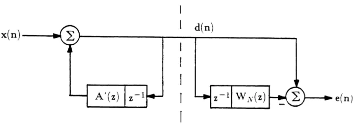
However, if the filter is configured in the "equation errorn form [23], as illustrated
in Figure 4.1, the resultant filter is always stable. This is because the equation
error form is not a true IIR form, with feedback paths. All signals are actually
filtered with unconditionally stable FIR filters. (The filter update algorithm's
sta-bility is not guaranteed, however!) Additionally, since this form is linear in the
filter parameters (tap weights), a unique LS solution is always available [23]. The
output of the unknown process is filtered, as well as the input signal, to produce an
Unknown
System
e(n)
B(z)
A(z)
estimate of the output of the system. The error of this estimate can be used to adjust the parameters of the model (filter) in order to minimize the LS error of the estimate.
The Fast Transversal Filter (FTF) algorithm
[32)
is a fast (order N), recur-sive, least squares algorithm. A!J such, it computes the LS filter solution in an extremely efficient manner. A multi-channel version of this algorithm allows mul-tiple input channels and mulmul-tiple output channels. In Chapter 3, the multi-channel FTF algorithm was extended to the case where various input multi-channels might have different filter orders. The two input channel case of this algorithm was shown to require 12N+
27 multiply or divide operations per recursive time update, where N is the total number of filter taps. In this chapter, we show how the general order, two input channel FTF algorithm can be applied to the problem of ARMA system identification. This configuration is also the one used for decision-directed equalization or echo cancellation, and hence has important appli-cations. For these applications, we will show that a computational savings of2N
+
1 operations per update can be achieved.Consider a two input channel joint process predictor, where now one of the input channels is connected to the unit-delayed'[ joint process signal, d(n). This is depicted in Figure 4.2. The indicated computational savings result since the
,-....
Q ~
' - ' " c:
::E
---~ ~~
...---....
d
"'---"
>.
-
IN
,-..
c:
...-.... '--'"
=
~' - '
-0
r ':
- - - I
I
ffJi
I
I
~
NI
o ~
Icl:
~
I
I
~
I
I
~
I
I
~
o
I
l~
.,
N
II
~
ar
IL_ - __
-.J
internal structure of the FTF algorithm requires the recursive computation of for-ward and backfor-ward predictors for the input channels. Because the ultimate goal of the joint process algorithm is the forward prediction of the desired signal, it should seem reasonable that the forward predictor for the unit-delayed desired signal (one of the input channels) is related to the joint process filter. This will be proven. Similarly, errors associated with these filters are related. These relationships are exploited to obtain the indicated computational reduction. The reduction avail-able with this special configuration will also apply to the Fast Kalman and the F AEST fast LS algorithms, which also use forward predictors of the input chan-nels.t This had not previously been recognized for applications of these algorithms.
4.2. ARMA System Identification
If a finite order, rational spectral model is postulated for an unknown linear system, with input {x(n)} and output {d(n)}, the system transfer function can be expressed in the z-domain as
Dl
z) bo
+
bIZ-I+ ... +
bL_1Z-L+1H(z)
=~X(
)
= -I -MZ 1 - alz _ ... - aMz
The roots of the numerator and denominator polynomials of
H(z)
correspond to the zeroes and poles of the system transfer function. This relationship is expressed in the time domain as an autoregressive-moving average (ARMA) differencetion
£-1 M
d(n)
=
~ bix(n-i)+
2:
aid(n-i)..=0
.=1(4.1)
Thus, it is assumed that there is also an additive uncorrelated noise term, and that the zero and pole polynomial orders Land M are known. This equation suggests a
form for the estimate of the joint process {d (n)} at time n that is linear in filter parameters available at time n:
A £-1 M
d(nln) =
2:
~i(n)x(n-i)+
~ Q:i(n)d(n-i),i=0 i=1
(4.2)
where cxi(n) and ~i(n) are adaptive weighting coefficients evaluated at time n. A prediction error is then
e(nln)
=d(n) - d(nln).
Note that the prediction in (4.2) is formed from a linear combination of previous {d (n)} rather than a regression on
{d (
n In)}. This is sometimes called the nequa-tion error" formulaequa-tion [23], and permits a tractable soluequa-tion to the LSproblem.
Table 4.1
Definitions for the Two-Channel Fast Transversal Configuration
Vectors and Matrices
1 (NX 1) zN(i)
=
[xl(i), yZ(i)]T, with L +M=
N 2 (LX 1) xL(i)=
[x(i), x(i-l), ... , x(i-L +1))T3 (MX1) YM(i)
=
[y(i), y(i-l),···, y(i-M+l)]T4 (n XI) x(n)
=
[x(I), x(2),···, x(n)]T 5 (n x1) y(n) = [y(l), y(2),···, y(n)]T6 (n x 2) z(n)
=
[x(n), y(n)]; zb(n)=
[z-Lx(n), z-My(n)] 7(2
x1) z(n)=
[x(n), y(n)]T; zb(n)=
[x(n-L), y(n-M)]T 8 (n XN) Zo(n)=
[zox(n), .. , z-L+lx(n),.y(n), .. ,z-M+ly(n)) 9 (n XN) Zl(n)=
[z-lx(n), .. , z-Lx(n), z-ly(n), .. , z-My(n)]Operators
10 (n x n) P(n)
=
Z(n)[ZT(n)Z(n)]-lZT(n) projection 11 (NX n) K(n)=
[ZT(n)Z(n)]-lZT(n) transversal filterTransversal Filters
12 (NX 1) wN(n)
=
Ko{n)d(n) joint process predictor 13 (Nx2) fN{n)=
K1{n)z(n) forward predictor 14 (Nx2) bN(n)=
KO(n)zb(n) backward predictor 15 (NX 1) gN(n)=
Ko(n)7T(n) gain (unit predictor) 16 (NX 1) cN(n)=
)'-l(n)gN(n) normalized gainPrediction Errors 17 (1X1) e(nln-l)= d(n)- wJ(n-l)zN(n) 18 (1X1) e(nln)
=
d(n) - wJ(n)zN(n)19 (2x 1) ef (n
In -
1)=
Z (n ) -r
Z(n - 1)zN(n - 1)20 (2x 1) ef(nln)= z(n) - rZ(n)zN(n-1)
21 (2x 1) eb(n
I
n - 1)=
zb (n ) - bZ(n - 1)ZN(n )22
(2x 1) eb(n In)=
zb(n) - bZ(n)zN(n)23 (1 x
i)
-y(n)=
1-gZ(n)zN(n)The scalar prediction error now can be described in vector notation as
~ T
e(nln)
=
d(n) - d(nln) = d(n) - WN(n)zN(n)where both data channels are collected into the(N xi )vector
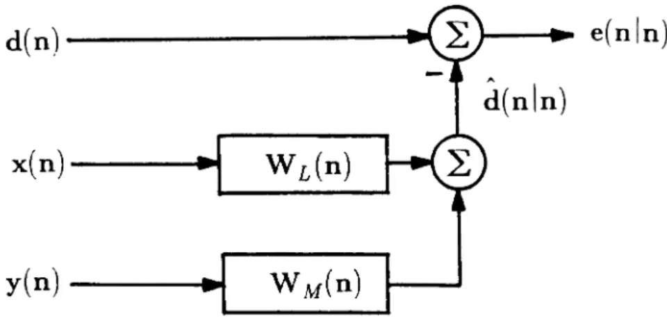
(4.3)
ZN(n)
=
[d:~~~1}l,
L+M=N, (4.4)and the (Nx
i)
joint process prediction filter W N( n) is partitioned into twopor-tions of lengths Land M that operate on the input and output processes,
respec-tively.
The prediction errors can be expressed as a vector which accumulates the scalar error at each time increment:
e(nln)
=
d(n) - d(nln)
=
d(n) - ZO(n)wN(n)
where now an (n XN) matrix of input data is createdZo(n)
=
(Xo(n),D1(n))
= [x(n), z-lx(n),··· ,z-L+lx(n), z-ld(n),··· ,z-Md(n)]
(4.5)
x(l) 0
x(2) x(l)
x(3) x(2)
=
x(n) x(n-l)
0
I
0 0 0I
d(l)
0I
d(2)
d(l)
x(l)
I
d(l)
I
x(n-L+l)
I
d(n-l) d(n-2) .d(n-M)
prediction filter, fN(n). This filter vector contains two length N columns, each corresponding to separate forward prediction filters for one of the input channels. For general input channel x (n) and y(n), the two columns of the filter are desig-nated:
(N
X2) fN(n) = [f~(n), fN(n)]or in this ARMA modeling case, where y(n) = z -ld( n ),
(NX2) rN(n) = [fN(n), rt(n)].
(4.6)
(4.7)
Similarly, the forward prediction error vector containing the scalar error associated with each subfilter is expressed:
(2X
l )
ef(nln)=
[eJ(nln), ef(nln)]TFrom Table4.1.13, the forward prediction filter is given as
fN{n) =
K1(n)z(n)
=
K1(n)[x(n), z-ld(n)],and thus
rt(n)
=
K1(n)z-ld(n).However, from Table 4.1.9
(4.8)
(4.9)
Zl(n) = [Zo(:T_1)]. (4.10)
By direct substitution of (4.10) into the definition for the transversal filter
opera-tor, (4.1.11), it is easily shown that
K1(n)
=[0, K o(n-l)]
(4.11)which relates operators for time delayed signals. Substituting this identity into
f~(n)
=[0,
Ko(n-l)]
[d(nO-1)] = Ko(n-l)d(n-l),
and, using definition (4.1.12)
(4.12)
f~(n)
=
wN(n-1). (4.13)Thus, it is shown that the optimal LS forward predictor for the delayed output
sig-nal is the same as the optimal joint process predictor from the previous iteration!
This is proven since the subspace of projection, Zo(n-1), is the same in both cases. This is intuitively clear if it is realized that the joint process filter is a forward
predictor of the desired signal d(n). The algorithm internally also requires a
for-ward prediction of each input channel.
Applying the identity of (4.13), a similar connection is readily shown between
the forward prediction errors associated with the respective filters:
e
f(
n In)=
e(n-11
n-1) ,
e
f(
nI
n -1)
=
e (n -11
n -2) .
(4.14a,b) The relationships of (4.13) and (4.14) create a significant reduction in thenumber of computations required to implement the fast transversal ARMA
predic-tor, compared to the standard 2-channel joint predictor case. The fact that several
necessary quantities are available from the preceding iteration allows a 2N
+
1reduction in operations. The savings result since one half of the (Nx
2)
forward prediction filter no longer needs to be computed; also one element of the (2x
i)
for-ward prediction error, normally computed by inner product, is also directlyrela
![Figure 4.1 Equation Error (after Astrom[23])](https://thumb-us.123doks.com/thumbv2/123dok_us/1178326.1148163/53.810.141.643.624.868/figure-equation-error-after-astrom.webp)