Coupled Structure (FE) & Fluid Flow (FV) Analysis for Vortex Induced Vibration

(1)

Coupled structure (FE) and fluid flow (FV) analysis for vortex induced vibrations

S. Patil ~), A. Murthy ~), Y. Dagba 2), A. Tripathi 2)

1) Fluidyn, Bangalore, India

2) Transoft International, Saint-Denis, France

A B S T R A C T

Fuel elements or any other tubular structure submerged in a fluid tank may be excited by seismic loading generating resonating response of vortex induced vibrations. High-speed interaction between two structures or a structure and a fluid requires simultaneous modeling of large deformations of structures and shock propagation in fluids. Modeling of varying flow regimes and boundary conditions in fluids is better managed by finite volumes, however, modelling of structural deformations is usually better done with finite elements. However, until now, available softwares have been using exclusively one of the two methods to model both fluids and structures,

fluidyn-FSI,

probably the only commercially available software of its kind. offers simultaneous use of both structures finite elements (for structures) and finite volumes (for fluid) formulations implemented inside the same solver.

A validation analysis has been done to simulate the structural deformations, modeled in finite elements and coupled in time domain with the surrounding fluid flow in finite volumes. The results in the Reynolds number range of 1000 to 125000 have been compared with the published experimental in-line and cross-line frequencies as well as drag coefficients although only results at Re = 1000 are shown here. The Strouhal number is also found to be very close to the estimates. The demonstrated software capability to adapt the fluid mesh to the displacements of the structure allows to keep a relatively low mesh density in the strong gradients zones, such as vortices and the boundary layer around the cylinder, thus ensuring a better precision of the results.

The same studies carded on for other kind of cylinders (square or variable cross-section) and for other flow configurations have shown similar results. The use of a solver capable of strong coupling between the fluid model and the structure model remains the best way to approach the modelisation of these phenomena. The coupled approach is made available for general usage influidyn-FSI software platform and has been used for other applications

I N T R O D U C T I O N

High-speed interaction between two structures or a structure and a fluid requires simultaneous modeling of large deformations of structures and shock propagation in fluids. On one hand, modeling of varying flow regimes and boundary conditions in fluids is better managed by finite volumes. Physical representation is also easier because results do not suffer from the numerical distorsion related to the shape function of the finite elements. On the other hand, modelling of structural deformations is usually better done with finite elements because the structural tridimensional complexities are difficult to follow in finite volumes. It allows also for larger integration time-steps. However, until now, available softwares have been using exclusively one of the two methods to model both fluids and structures. Therefore the user had to accept approximate solutions either in fluids or structures depending on the method preferred.

fluidyn-FSI,

probably the only commercially available software of its kind. offers simultaneous use of both structures finite elements (for structures) and finite volumes (for fluid) formulations implemented inside the same solver. Therefore all kinds of structural state equations, laws of plastifications, damage and spalling, as well as all kinds of fluid state equations and boundary conditions, can be introduced without any hesitation. Boundary conditions between finite volumes and finite elements are exchanged automatically.

After a quick overview of

fluidyn-FSI

software, the case of the propagation of a crack in a cylindrical tank is presented. The geometry, meshes, boundary and initial conditions are described, before presenting and analyzing the results.

T H E S O F T W A R E

fluidyn-FSI

gathers, inside one solver, two models : a fluid solver in finite volumes and a structural solver in finite elements. The two solvers are coupled through an automatic boundary information exchange. A more complete description of the solvers can be found in [ 1].

Fluid m o d e l

The fluid model is based on

fluidyn-NS

software, designed to solve the Navier-Stokes equations to compute internal and external flows in complex 3D geometries with high-order numerical schemes. Various finite volume schemes are available (Roe, Van Leer, Roe Preconditioned, AUSM, Partial Donor Cell, HLLC, etc) and can be chosen according to the kind of application encountered. The numerical precision of the schemes can be as high as the third order and the mesh can be structured, unstructured or hybrid. Several equations of state are also available, including two-

SMiRT 16, Washington DC, August 2001

Paper # 2010

(2)

phase equations of state for phase change or for two-phase dispersed flows. Flows range from incompressible (e.g. sloshing) to highly compressible phenomena (e.g. detonation). Simultaneous presence of multiple fluids is possible and, in certain conditions, two or more numerical schemes can be used for different parts of a same domain [2], [3].

Structural model

Though

fluidyn-FSI

offers the possibility to model the structures in Finite Volumes whenever the strain rate is very high (such as in the case of target penetration), the finite element structural model is generally used for the modelling of complex 3-D structures [4],[5]. The elements available for general use are beams, thin plates and tetrahedrons. The formulation of high strain rates and displacements is constantly updated and has been validated through nuclear and aerospace industries cases. The material equation of state can be elastic, elasto-plastic, piecewise stress-strain curve with isotropic or orthotropic behaviour, etc., coupled with a material database. Generally admitted plastification and spalling laws, such as Steinberg, Guinan and Johnson & Cook, in which temperature and pressure effects, are also available. Stable timesteps for shell elements in particular are computed through the formulation of [6].

Coupling of fluids and structures

At the fluid/structure interface, the structural solver computes the corresponding deformations and structure velocities, taking into account the loads due to the fluid pressure. The fluid mesh adjusts itself to the new position of the structure while preserving continuity of the normal component of the velocity. The fluid remeshing is automatic and the fluid variables are redistributed. The new distribution of fluid nodes leads to a new pressure field in the fluid. This cycle is repeated till convergence. When explicit integration is used for the stress model, the stable timestep for integration may be smaller tahn the fluid timestep. This necessitates a finite number of substeps of the stress model to complete one cycle of fluid model. However, by using implicit integration, one cycle of the stress model is sufficient to reach the timestep of the fluid cycle.

D E S C R I P T I O N OF CASE

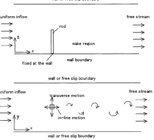
The simulation undertaken here deals with a fuel element fixed on the bottom of a tank and bottom and the vortex shedding behind it. The cylindrical tube forming the fuel element is fixed at the bottom and is subjected to a uniform flow. Vortices are generated behind the cylinder and are shedded (figure 1).

wall or free slip boundary

uniform inflow free stream

'> rod >

;T"

wake region

wall boundary

fixed at the wall

uniform inflow

>

f -

f

> x

t/•ansve

rs e motion

I r h - . r-~

in-line motion

fre e stre a m

>

(3)

The cylindrical tube is made out of steel and is 0.135 m long. Its diameter is 0.01m. The computational domain is 0.25 m in the x-direction and 0.1 m in the z-direction (figure 2).

5d

A

.W."

5d 20d

. < . ... . > < ... . ... . . >

I

1

I

0

I

0

I

i

I

i

I

Fig.2 Simulation d o m a i n (d = d i a m e t e r of cylinder)

M O D E L

A transient analysis is performed. Table 1 lists the computational parameters used.

Table 1. Structural m o d e l

Material

Integration scheme Equation of state Young modulus Poisson ratio Density

Steel Explicit Linear elastic

210 Gpa 0.3 7800 kg/m3

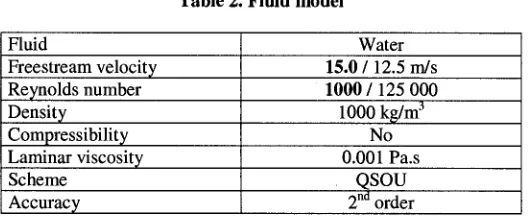
The flow is incompressible isothermal and laminar. Two cases of different Reynolds numbers were considered, although only the results of the first one are going to be presented in this paper.

Table 2. Fluid model

Fluid Water

Freestream velocity 15.0 / 12.5 m/s Reynolds number

Density Compressibility Laminar viscosity Scheme

Accuracy

1000 / 125 000

1000 kg/m 3 No 0.001 Pa.s

QSOU 2 nd order

M E S H

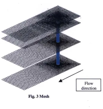
The mesh in figure 3 is composed by a total of 3200 cells. The mesh is refined around the tube. B O U N D A R Y C O N D I T I O N S

B o u n d a r y conditions for structure

The base of the cylinder is rigid, all nodes lying on Z-minimum plane are fixed for forces and moments. The top of the cylinder is left free to oscillate.

B o u n d a r y conditions for fluid

(4)

Fig. 3 Mesh

Flow direction

INITIAL CONDITIONS

At t = 0, the structure is at rest and the fluid is moving at the velocity of 15 m/s (or 12.5 m/s).

RESULTS AND DISCUSSION

Vortices generation and behavior of the tube

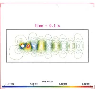
Figure 4 shows the contours of the velocity component in the y direction at various planes along the length of the tube (in pink), freezed at a certain time after stabilization has been reached. The vortices forming behind the tube can clearly be identified as alternate patches of red and blue (see also figure 5). The tridimensional structure of the vortex generation is demonstrated, since the slices of the velocity contours are not the same on all planes. This is shown also in figure 6 where a longitudinal slice has been made along the tube. The time period of vortex shedding, At, and frequency of vortex shedding, f, are found to be :.

At = 0.00322 s f = 310.6 Hz

It is observed that the in-line frequency (frequency of the drag coefficient

Cd)

is twice of the cross-line frequency (frequency of the lift coefficient C1). This observation is corroborated in literature [7].

V - v e l o c i t y

- ] ,50+000 - 4 , 7 4 - 0 0 ] 5 . 5 3 - 0 0 ] 1,50+000

(5)

F - 1

Time = 0 . I s

_ _

.. -. ,/, L. ,.--., _ . /-- ..

./ . .... ",, f ," :--. .'~/7. -..,/, .... .:. <..", i' --.. ", ,- --. ( .... ",

I .,' -.', '-.~)'.'/'::.:::'..'v 1,::--::::.!, ;,";7::~"~ ~, /.---..t,I - ".,", -- I ,'" "'. "

.-

(. (,:>

( '.-:hr.

i~!:!:;~;~):..,~%!,:::~:~_:!;~/@~;:i!g'i:d:!::iiiL:",;".(

',:,'',1,-

-./~

... " : ' ..- :.-' ', "----'~ f :--- .,'~ ', - '_ ")' L - " ..', " ... / ' - -." ~ "-" ,,

_ t t ". ,./ "-- '1 " ~ - ',, ) :, /

V - v e ' l o o t t y

- i ,20+001 -4.10+000 3.01+000 l , 11+001

I I .t ... tk,...1...,__S I . . . I ... ... i : . . ~ , i I

Fig. 5 slice along the x-axis at a particular plane of the V - c o m p o n e n t of the velocity . . .

I ,T'.~.."Z:- .... -' . . . . -- ~ : ..- - - .

,' ~i.-'.:': "!:~g%:;',;.7~:=-. ' , ; - _ = : . - , ,' ~ - -, . " _ ! _

I~i<.:':':@:,--::',',:f!,Isf,--.'~li "-, !i ,"--' I ;-",, ,

;

,Iilit ':q~,'~l,..:,\'4ti'ii',~ ".,v,,~fi[ ', i\ i i / ! I

c,--:',S'.ts'~.):~tt,: ',, ".:,: :::.",,~.;-. " .,'..'re,';'< . I_ ~'.', '. \ ~, '. ". ) '

) , , , ~ , . . . . . . ,~,,.k,,. ... -.,,,~.. ~,.,s . . . . ~ ~ , , ,

I ;~::.~.::.: :!~:' ":::.:, ','{".~,',%4:;:. ', "S.'.',V,;'~. ',' '.,',,',.';,'.:, '. J \','..", ". '; ", ', ', ~, '.

/ :~.: % ."d:,, '.'.:'kt'.t:,::~7,'-,, > ;h',','.i:':'); .. ',.' \"..'~, " ~,', ,",. ~'-, ; ", ":, , .I ", ," ,~!~ ~:%i!i::"::@i(>t.":<,i:!",':}iiil ': :>~;?;:':',-~",".', /', '

• :t: ., ,, Lb.-:.:;.<:, ? t, ;-:;... /, ! .,'; . _, /

V - v e l o c i t y

- 9 , 2 5 + 0 0 0 - 2 , 7 0 + 0 0 0 3.86+000 9 , 9 1 " 00{~ III .... J l . . . I II l _I ... : : : , ! ; : : ~ , ' : ~

Fig. 6 Slice along the z-axis at a particular plane of the V - c o m p o n e n t of the velocity

The in-line and transverse response of the cylinder are shown in figure 7. The transverse displacement is seen to be growing in time which is indicative of a lock-in and resonant behavior of the structure with the fluid. In figure 8, the maximum displacement of the structure. The fluid mesh follows the displacement of the structure.

vie. 0

0,6

D 0.4

i

B

x

E 0,l

0

3 0,11

1

Displacement

I

!! !;,

;i

/,,

,;,,,lii;./~/',!'''

"'"

~.,

I I I

0,06 0,12 0,i8 0,24 0,3 Time [xE-0l]

X corr~m of sliuaunl d i ~ c ~ a~ no~ 4519 (z---015) (W~ r ~ h )

vie, 2

Displacement

/ i! UY-'t~19 i! '~

o . ~ I - - - -t,-h

p

]

,-, /~ i i

t ol_~ /"~ i';;i! i

I " ' i ! ! f ~ i i E " zv; ~ : !

-..h

',s

~-o.~ • " ~i

I i I 71

0 , ~ 0,12 0,18 11.24 0,3

Time [x~-01]

Y c0mp~mt of SttUeturdl d i ~ n n n a at node 4519 (z-015) (W~h rnn~)

Fig. 7 In-line and transverse displacements of the tube in time

(6)

view 1 VP0

L

Fig. 8 M a x i m u m displacement of the tube

Drag coefficients

The draf coefficient is computed from the Eq. (1) •

where,

C d =

D

0.5pUooA

D =component of the resultant force parallel to the undisturbed initial velocity (U~) A= frontal area exposed by the body to the flow direction = ( d*l )

1 = length of cylinder

(1)

The evolution of drag coefficient on time is presented in Fig.9. The maximum and the minimum value of Cd are 1.257 and 1.0777 respectively. The average value of Cd is around 1.16735. Table 3 compares the computed values with the values taken from literature [7]

Cd

Drag C o e t £ i c i e n £ vs T i m e

1 . 2 4

1 , 2

1 . 1 6

1° 12

t .

'~

_ _¢/

!

i

-- / i

t t

( ?

,/

/

f

(

i

/

"\,

/

t

0.10105 0.1014 0.102 0.1026 0.1032 0.1038 O, 10427

Fig.9 : Evolution of drag coefficient in time

(7)

Table-3 Comparison of experimental and numerical Cd

Source Literature [7]

Reynolds Number (Re) 1000

Drag Coefficient (Cd) 1.00000

Simulation 1000 1.16735

Strouhal number :

The Strouhal number is computed from Eq. (2)

S t - f d U~o

(2)

Its value is found to be 0.207 which is in a good agreement with the theoretical value of 0.2 [7].

SUMMARY AND CONCLUSION

A new method of fluid/structure interaction has been used to compute the vortex-induced vibrations on a cylinder. The software capability to adapt the fluid mesh to the displacements of the structure allows to keep a relatively low mesh density in the strong gradients zones, such as vortices and the boundary layer around the cylinder, thus ensuring a better precision of the results.

The load exerted on the cylinder by the flow is non-uniform along its length. The vibration frequencies thus generated are variable with respect to the height and can be captured only if the structure displacements are followed by a complete remeshing of the domain around the cylinder along with a redistribution of the fluid variables onto the new mesh.

The drag coefficient and Strouhal number are in good agreement with previously published data. The in-line frequency is found out to be twice of cross-line frequency from the simulation, as was expected.

The same studies carried on for other kind of cylinders (square or variable cross-section) and for other flow configurations have shown similar results. The use of a solver capable of strong coupling between the fluid model and the structure model remains the best way to approach the modelisation of these phenomena.

REFERENCES

1. Stassinopoulos, A., Suresh, K. and Ramesh, T.C., "Numerical Modelling of conjugate heat transfer applications using a new 3D fluid-solid interaction approach," EUROTHERM, 1999.

2. Jameson, A., Baker, T.J. and Weatherbill, N.P., "Calculations of inviscid transonic flow over a complete aircraft",

AIAA 86-0103, 1986.

3. Roe, P.L., "Approximate Tiemann solvers, parameter vectors and difference schemes," Journal of Computational

Physics, Vol. 43, 1981, pp. 357-372.

4. Van Leer, B., "Flux vector splitting for Euler equations," Lecture Notes in Physics, Vol. 170, 1982, pp.507.

5. Kennedy, J.M., Belytschko, T. and Lin, J.I., "Recent developments in explicit finite element techniques and their applications to reactor structures," Journal of Nuclear Engineering and design, Vol. 97, 1986, pp. 343-354.

6. Fasoli-Stella, P. and Jones, A.V., Advanced Structural Dynamics, pp. 191-254, Applied Science Publishers, London, 1980.