Is CPU queue empty?
Is MCL = tarr
? b
b
b
b
2 1
2
4 5 6
3 3
9 6 9
7
MCL = tarr MCL = MCL + 1
CPU
A new arrival event occurs
A new arrival event occurs A departure event occurs
Yes
Yes No
Computer Simulation Techniques:
The de
fi
nitive introduction!
Computer Simulation Techniques:
The definitive introduction!
by
Harry Perros
Computer Science Department
NC State University
Raleigh, NC
TO THE READER…
This book is available for free download from my web site: http://www.csc.ncsu.edu/faculty/perros//simulation.pdf
Self-study: You can use this book to learn the basic simulation techniques by yourself! At the end of Chapter 1, you will find three examples. Select one of them and do the corresponding computer assignment given at the end of the Chapter. Then, after you read
each new Chapter, do all the problems at the end of the Chapter and also do the computer assignment that corresponds to your problem, By the time you reach the end of
the book, you will have developed a very sophisticated simulation model! You can use any high-level programming language you like.
Errors: I am not responsible for any errors in the book, and if you do find any, I would appreciate it if you could let me know ([email protected]).
Acknowledgment: Please acknowledge this book, if you use it in a course, or in a project, or in a publication.
Copyright: Please remember that it is illegal to reproduce parts of this book or all of the book in other publications without my consent.
I would like to thank Attila Yavuz and Amar Shroff for helping me revise Chapters 2 and 4 and also my thanks to many other students for their suggestions.
Enjoy!
TABLE OF CONTENTS
Chapter 1. Introduction, 1
1.1 The OR approach, 1
1.2 Building a simulation model, 2
1.3 Basic simulation methodology: Examples, 5 1.3.1 The machine interference model, 5 1.3.2 A token-based access scheme, 11 1.3.3 A two-stage manufacturing system, 18 Problems, 22
Computer assignments, 23
Chapter 2. The generation of pseudo-random numbers, 25 2.1 Introduction, 25
2.2 Pseudo-random numbers, 26 2.3 The congruential method, 28
2.3.1 General congruencies methods, 30 2.3.2 Composite generators, 31
2.4 Tausworthe generators, 31
2.5 The lagged Fibonacci generators, 32 2.6 The Mercenne Twister, 33
2.7 Statistical tests of pseudo-random number generators, 36 2.7.1 Hypothesis testing, 37
2.7.2 Frequency test (Monobit test), 38 2.7.3 Serial test, 40
2.7.4 Autocorrelation test, 42 2.7.5 Runs test, 43
2.7.6 Chi-square test for goodness of fit, 45 Problems, 45
Computer assignments, 46
Chapter 3. The generation of stochastic variates, 47 3.1 Introduction, 47
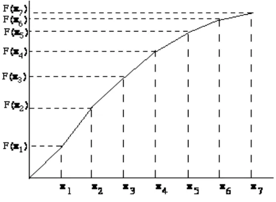
3.2 The inverse transformation method, 47
3.3 Sampling from continuous-time probability distribution, 49 3.3.1 Sampling from a uniform distribution, 49
3.3.3 Sampling from an Erlang distribution, 51 3.3.4 Sampling from a normal distribution, 53
3.4 Sampling from a discrete-time probability distribution, 55 3.4.1 Sampling from a geometric distribution, 56
3.4.2 Sampling from a binomial distribution, 57 3.4.3 Sampling from a Poisson distribution, 58 3.5 Sampling from an empirical probability distribution, 59
3.5.1 Sampling from a discrete-time probability distribution, 59 3.5.2 Sampling from a continuous-time probability distribution, 61 3.6 The Rejection Method, 63
3.7 Monte-Carlo methods, 65 Problems, 66
Computer assignments, 68 Solutions, 69
Chapter 4. Simulation designs, 71 4.1 Introduction, 71
4.2 Event-advance design, 71 4.3 Future event list, 73 4.4 Sequential arrays, 74 4.5 Linked lists, 75
4.5.1 Implementation of a future event list as a linked list, 76 a. Creating and deleting nodes, 76
b. Function to create a new node, 78 c. Deletion of a node, 79
d. Creating linked lists, inserting and removing nodes, 79 e. Inserting a node in a linked list, 80
f. Removing a node from the linked list, 83 4.5.2 Time complexity of linked lists, 86 4.5.3 Doubly linked lists, 87
4.6 Unit-time advance design, 87 4.6.1 Selecting a unit time, 90 4.6.2 Implementation, 91
4.6.3 Event-advance vs. unit-time advance, 91 4.7 Activity based simulation design, 92
4.8 Examples, 94
4.8.1 An inventory system, 94 4.8.2 Round-robin queue, 97 Problems, 101
Computer assignments, 102
Appendix A: Implementing a priority queue as a heap, 104 A.1 A heap, 104
A.4 Implementing a future event list as a priority queue, 113
Chapter 5. Estimation techniques for analyzing endogenously created data, 115 5.1 Introduction, 115
5.2 Collecting endogenously created data, 115 5.3 Transient state vs. steady-state simulation, 118
5.3.1 Transient-state simulation, 118 5.3.2 Steady-state simulation, 119
5.4 Estimation techniques for steady-state simulation, 120
5.4.1 Estimation of the confidence interval of the mean of a random variable, 120
a. Estimation of the autocorrelation coefficients, 123 b. Batch means, 128
c. Replications, 129
d. Regenerative method, 131
5.4.2 Estimation of other statistics of a random variable, 138 a. Probability that a random variable lies within a fixed
interval, 138
b. Percentile of a probability distribution, 140 c. Variance of the probability distribution, 141 5.5 Estimation techniques for transient state simulation, 142
5.6 Pilot experiments and sequential procedures for achieving a required accuracy, 143
5.6.1 Independent replications, 144 5.6.2 Batch means, 144
Computer assignments, 145
Chapter 6. Validation of a simulation model, 149 Computer assignments, 150
Chapter 7. Variance reduction techniques, 155 7.1 Introduction, 155
7.2 The antithetic variates technique, 156 7.3 The control variates technique, 162 Computer assignments, 165
Chapter 8. Simulation projects, 166
CHAPTER 1:
INTRODUCTION
1.1 The OR approach
The OR approach to solving problems is characterized by the following steps:
1. Problem formulation
2. Construction of the model
3. Model validation
4. Using the model, evaluate various available alternatives (solution)
5. Implementation and maintenance of the solution
The above steps are not carried out just once. Rather, during the course of an OR
exercise, one frequently goes back to earlier steps. For instance, during model validation
one frequently has to examine the basic assumptions made in steps 1 and 2.
The basic feature of the OR approach is that of model building. Operations Researchers like to call themselves model builders! A model is a representation of the
structure of a real-life system. In general, models can be classified as follows: iconic, analogue, and symbolic.
An iconic model is an exact replica of the properties of the real-life system, but in
smaller scale. Examples are: model airplanes, maps, etc. An analogue model uses a set of
properties to represent the properties of a real-life system. For instance, a hydraulic
system can be used as an analogue of electrical, traffic and economic systems. Symbolic
such as mathematical equations and computer programs. Obviously, simulation models
are symbolic models.
Operations Research models are in general symbolic models and they can be
classified into two groups, namely deterministic models and stochastic models. Deterministic models are models which do not contain the element of probability.
Examples are: linear programming, non-linear programming and dynamic programming.
Stochastic models are models which contain the element of probability. Examples are:
queueing theory, stochastic processes, reliability, and simulation techniques.
Simulation techniques rely heavily on the element of randomness. However,
deterministic simulation techniques in which there is a no randomness, are not
uncommon. Simulation techniques are easy to learn and are applicable to a wide range of
problems. Simulation is probably the handiest technique to use amongst the array of OR
models. The argument goes that "when everything else fails, then simulate". That is,
when other models are not applicable, then use simulation techniques.
1.2 Building a simulation model
Any real-life system studied by simulation techniques (or for that matter by any other OR
model) is viewed as a system. A system, in general, is a collection of entities which are
logically related and which are of interest to a particular application. The following
features of a system are of interest:
1. Environment: Each system can be seen as a subsystem of a broader system. 2. Interdependency: No activity takes place in total isolation.
3. Sub-systems: Each system can be broken down to sub-systems.
4. Organization: Virtually all systems consist of highly organized elements or components, which interact in order to carry out the function of the system.
When building a simulation model of a real-life system under investigation, one
does not simulate the whole system. Rather, one simulates those sub-systems which are
related to the problems at hand. This involves modelling parts of the system at various
levels of detail. This can be graphically depicted using Beard's managerial pyramid as
shown in Figure 1.1. The collection of blackened areas form those parts of the system
that are incorporated in the model.
Figure 1.1: Beard's managerial pyramid
A simulation model is, in general, used in order to study real-life systems which
do not currently exist. In particular, one is interested in quantifying the performance of a
system under study for various values of its input parameters. Such quantified measures
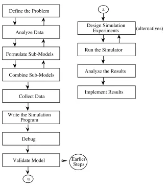
of performance can be very useful in the managerial decision process. The basic steps
involved in carrying out a simulation exercise are depicted in Figure 1.2.
All the relevant variables of a system under study are organized into two groups.
Those which are considered as given and are not to be manipulated (uncontrollable variable) and those which are to be manipulated so that to come to a solution
Figure 1.2: Basic steps involved in carrying out a simulation study.
Another characterization of the relevant variables is whether they are affected or
not during a simulation run. A variable whose value is not affected is called exogenous. A variable having a value determined by other variables during the course of the simulation
is called endogenous. For instance, when simulating a single server queue, the following variables may be identified and characterized accordingly.
Exogenous variables
1. The time interval between two successive arrivals.
2. The service time of a customer.
3. Number of servers. Define the Problem
Analyze Data
Formulate Sub-Models
Combine Sub-Models
Collect Data
Write the Simulation Program
Debug
Validate Model
Design Simulation Experiments
Run the Simulator
Analyze the Results
Implement Results
(alternatives) a
a
4. Priority discipline.
Endogenous variables
1. Mean waiting time in the queue.
2. Mean number of customers in the queue.
The above variables may be controllable or uncontrollable depending upon the
experiments we want to carry out. For instance, if we wish to find the impact of the
number of servers on the mean waiting time in the queue, then the number of servers
becomes an controllable variable. The remaining variables-the time interval between two
arrivals and the service time, will remain fixed. (uncontrollable variables)
Some of the variables of the system that are of paramount importance are those
used to define the status of the system. Such variables are known as status variables. These variables form the backbone of any simulation model. At any instance, during a
simulation run, one should be able to determine how things stand in the system using
these variables. Obviously, the selection of these variables is affected by what kind of
information regarding the system one wants to maintain.
We now proceed to identify the basic simulation methodology through the means
of a few simulation examples.
1.3 Basic simulation methodology: Examples
1.3.1 The machine interference problem
Let us consider a single server queue with a finite population known as the machine interference problem. This problem arose originally out of a need to model the behavior of machines. Later on, it was used extensively in computer modelling. Let us consider M
machines. Each machine is operational for a period of time and then it breaks down. We
assume that there is one repairman. A machine remains broken down until it is fixed by
non-preemptive. Obviously, the total down time of a machine is made up of the time it
has to "queue" for the repairman and the time it takes for the repairman to fix it. A
machine becomes immediately operational after it has been fixed. Thus, each machine
follows a basic cycle as shown in figure 1.3, which is repeated continuously.
Figure 1.3: The basic cycle of a machine.
In general, one has information regarding the operational time and the repair time
of a machine. However, in order to determine the down time of a machine, one should be
able to calculate the queueing time for the repairman. If this quantity is known, then one
can calculate the utilization of a machine. Other quantities of interest could be the
utilization of the repairman.
Figure 1.4: The machine interference problem.
Let us now look at the repairman's queue. This can be visualized as a single server
queue fed by a finite population of customers, as shown in figure 1.4
For simplicity, we will assume that the operational time of each machine is equal
to 10 units of time. Also, the repair time of each machine is equal to 5 units of time. In
other words, we assume that all the machines have identical constant operational times.
Finite Population of Machines
They also have identical and constant repair times. (This can be easily changed to more
complicated cases where each machine has its own random operational and repair times.)
The first and most important step in building a simulation model of the above
system, is to identify the basic events whose occurrence will alter the status of the system. This brings up the problem of having to define the status variables of the above
problem. The selection of the status variables depends mainly upon the type of
performance measures we want to obtain about the system under study.
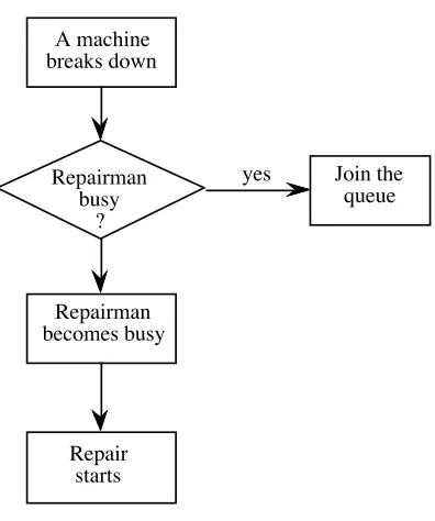
Figure 1.5: An arrival event.
In this problem, the most important status variable is n, the number of broken
down machines, i.e., those waiting in the queue plus the one being repaired. If n=0, then
we know that the queue is empty and the repairman is idle. If n=1, then the queue is
empty and the repairman is busy. If n>1, then the repairman is busy and there are n-1
broken down machines in the queue. Now, there are two events whose occurrence will
cause n to change. These are:
1. A machine breaks down, i.e., an arrival occurs at the queue. A machine
breaks down
Repairman busy
?
yes
Repairman becomes busy
Repair starts
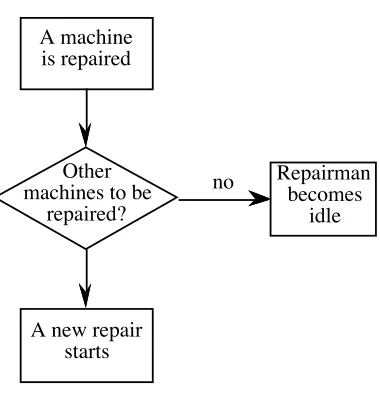
2. A machine is fixed, i.e., a departure occurs from the queue.
The flow-charts given in figures 1.5, and 1.6 show what happens when each of
these events occur.
Figure 1.6: A departure event.
In order to incorporate the above two basic events in the simulation model, we
need a set of variables, known as clocks, which will keep track of the time instants at which an arrival or departure event will occur. In particular, for this specific model, we
need to associate a clock for each machine. The clock will simply show the time instant
at which the machine will break down, i. e., it will arrive at the repairman's queue.
Obviously, at any instance, only the clocks of the operational machines are of interest. In
addition to these clocks, we require to have another clock which shows the time instant at
which a machine currently being repaired will become operational, i.e., it will cause a
departure event to occur. Thus, in total, if we have m machines, we need m+1 clocks.
Each of these clocks is associated with the occurrence of an event. In particular, m clocks
are associated with m arrival events and one clock is associated with the departure event.
A machine is repaired
no
A new repair starts
Repairman becomes
idle Other
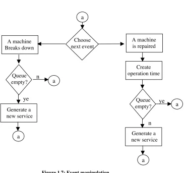
In addition to these clocks, it is useful to maintain a master clock, which simply keeps track of the simulated time.
The heart of the simulation model centers around the manipulation of these
events. In particular, using the above clocks, the model decides which of all the possible
events will occur next. Then the master clock is advanced to this time instant, and the
model takes action as indicated in the flow-charts given in figures 1.5 and 1.6. This event
manipulation approach is depicted in figure 1.7
.
Figure 1.7: Event manipulation.
We are now ready to carry out the hand simulation shown below in table 1. Let us
assume that we have 3 machines. Let CL1, CL2, and CL3 be the clocks associated with
machine 1, 2, and 3 respectively (arrival event clocks). Let CL4 be the clock associated Choose
next event a
A machine Breaks down
A machine is repaired
Create operation time
Generate a new service
Queue
empty? yes a
n o
a Generate a
new service Queue
empty? no
ye s
a
with the departure event. Finally, let MC be the master clock and let R indicate whether
the repairman is busy or idle. We assume that at time zero all three machines are
operational and that CL1=1, CL2=4, CL3=9. (These are known as initial conditions.)
MC CL1 CL2 CL3 CL4 n
0 1 4 9 - 0 idle
1 - 4 9 6 1 busy
4 - - 9 6 2 busy
6 16 - 9 11 1 busy
9 16 - - 11 2 busy
11 16 21 - 16 1 busy
16 - 21 26 21 1 busy
Table 1: Hand simulation for the machine interference problem
We note that in order to schedule a new arrival time we simply have to set the
associated clock to MC+10. Similarly, each time a new repair service begins we set
CL4=MC+5. A very important aspect of this simulation model is that we only check the
system at time instants at which an event takes place. We observe in the above hand
simulation that the master clock in the above example gives us the time instants at which
something happened (i.e., an event occurred). These times are: 0, 1, 4, 6, 9, 11, 16, ... We
note that in-between these instants no event occurs and, therefore, the system's status
remains unchanged. In view of this, it suffices to check the system at time instants at
which an event occurs. Furthermore, having taken care of an event, we simply advance
the Master clock to the next event which has the smallest clock time. For instance, in the
above hand simulation, after we have taken care of a departure of time 11, the simulation
will advance to time 16. This is because following the time instant 11, there are three
events that are scheduled to take place in the future. These are: a) arrival of machine 1 at
time 16; b) arrival of machine 2 at time 21; and c) a departure of machine 3 at time 16.
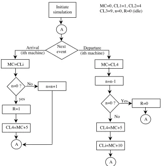
The above simulation can be easily done using a computer program. An outline of
the flow-chart of the simulation program is given in figure 1.8. The actual
implementation of this simulation model is left as an exercise.
Figure 1.8: A flowchart of the simulation program.
1.3.2 A token-based access scheme
We consider a computer network consisting of a number of nodes interconnected via a
shared wired or wireless transport medium, as shown in figure 1.9. Access to the shared
medium is controlled by a token. That is, a node cannot transmit on the network unless it
has the token. In this example, we simulate a simplified version of such an access
scheme, as described below.
Initiate simulation
A
Next event
MC=0, CL1=1, CL2=4 CL3=9, n=0, R=0 (idle)
Arrival
(ith machine) (ith machine) Departure
MC=CLi MC=CL4
n=0 ?
R=1 yes
No n=n+1
CL4=MC+5
A
n=n-1
n=0 ? Yes R=0
A CL4=MC+5
No
CLi=MC+10
Figure 1.9: Nodes interconnected by a shared medium
There is a single token that visits the nodes in a certain logical sequence. The nodes are
logically connected so that they form a logical ring. In the case of a bus-based or
ring-based wireline medium, the order in which the nodes are logically linked may not be the
same with the order in which they are attached to the network. We will assume that the
token never gets lost. A node cannot transmit unless it has the token. When a node
receives the token, from its previous logical upstream node, it may keep it for a period of
time up to T. During this time, the node transmits packets. A packet is assumed to consist
of data and a header. The header consists of the address of the sender, the address of the
destination, and various control fields. The node surrenders the token when: a) time T
has run out, or b) it has transmitted out all the packets in its queue before T expires, or c)
it receives the token at a time when it has no packets in its queue to transmit. If time T
runs out and the node is in the process of transmitting a packet, it will complete the
transmission and then it will surrender the token. Surrendering the token means, that the
node will transmit it to its next downstream logical neighbor.
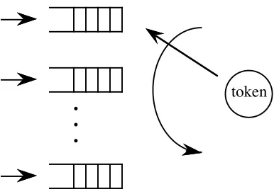
Conceptually, this network can be seen as comprising of a number of queues, one
per node. Only the queue that has the token can transmit packets. The token can be seen
as a server, who switches cyclically between the queues, as shown in figure 1.10. Once
the token is switched to a queue, packets waiting in this queue can be transmitted on the
network. The maximum time that a queue can keep the token is T units of time, and the
token is surrendered following the rules described above. The time it takes for the token
to switch from one queue to the next is known as switch-over time. Such queueing
systems are referred to as polling systems, and they have been studied in the literature
Figure 1.10. The conceptual queueing system.
It is much simpler to use the queueing model given in figure 1.10 when
constructing the simulation model of this access scheme. The following events have to be
taken into account in this simulation. For each queue, there is an arrival event and service
completion event. For the token, there is a time of arrival at the next queue event and the
time when the token has to be surrendered to the next node, known as the time-out. For
each queue, we keep track of the time of arrival of the next packet, the number of
customers in the queue, and the time a packet is scheduled to depart, if it is being
transmitted. For the token, we keep track of the time of arrival at the next queue, the
number of the queue that may hold the token, and the time-out.
In the hand simulation given below we assume that the token-based network
consists of three nodes. That is, the queueing system in figure 1.10 consists of three
queues. The inter-arrival times to queues 1, 2, and 3 are constant and they are equal to 10,
15, and 20 unit times respectively. T is assumed to be equal to 15 unit times. The time it
takes to transmit a packet is assumed to be constant equal to 6 unit times. The switch over
time is equal to 1 unit time. For initial conditions we assume that the system is empty at
time zero, and the first arrival to queues 1, 2, and 3 will occur at time 2, 4 and 6
respectively. Also, at time zero, the token is in queue 1. In case when an arrival and a
departure occur simultaneously at the same queue, we will assume that the arrival occurs
first. In addition, if the token and a packet arrive at a queue at the same time, we will
assume that the packet arrives first.
The following variables represent the clocks used in the flow-charts:
a. MC: Master clock
b. ATi: Arrival time clock at queue i, i=1,2,3 c. DTi: Departure time clock from queue i, i=1,2,3 d. TOUT: Time out clock for token
e. ANH: Arrival time clock of token to next queue
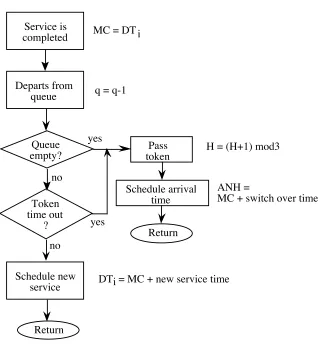
The logic for each of the events in this simulation is summarized in figures 1.11 to
1.14. Specifically, in figure 1.11 we show what happens when an arrival occurs, figure
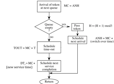
1.12 deals with the case where a service is completed at queue i, figure 1.13 describes the action taken when a time-out occurs, and figure 1.14 summarizes the action taken when
the token arrives at a queue.
The set of all possible events that can occur at a given time in a simulation is
known as the Figure 1.13 event list. This event-list has to be searched each time in order to locate the next event. This event manipulation forms the basis of the simulation, and it
is summarized in figure 1.15.
Figure 1.11: Arrival event at queue i. Arrival
occurs
Join the queue
Schedule Next Arrival
Arrivals
Return
MC=ATi
qi = qi + 1
ATi = MC + new
Figure 1.12: Service completion at queue i.
Figure 1.13 : Time-out of token
Service is completed
Departs from queue
Return
Pass token MC = DT
q = q-1
H = (H+1) mod3
Schedule new service
Schedule arrival time Queue
empty?
Token time out
?
Return
ANH =
MC + switch over time
DT = MC + new service time yes
no
no
i
i yes
Time-out occurs
Return
This means that node is still transmitting.
Figure 1.14 : Arrival of token at next queue.
Figure 1.15 : Event manipulation. Initialize
simulation
End
i. e. search event list for smallest number
If new events are scheduled update next
event
Is simulation
over ? Take appropriate
action Locate next event
no
yes
The hand simulation is given in table 2.
Queue 1 Queue 2 Queue 3 Token
MC Arr Clock Depart Clock Queue size Arr Clock Depart Clock Queue size Arr Clock Depart Clock Queue size Node No Time Out Clock Arrival Next Node
0 2 0 4 0 6 0 1 1
1 2 0 4 0 6 0 2 2
2 12 1 4 0 6 0 3 3
3 12 9 1 4 0 6 0 1 18
4 12 9 1 19 1 6 0 1 18
6 12 9 1 19 1 26 1 1 18
9 12 0 19 1 26 1 1 10
10 12 0 19 16 1 26 1 2 25
12 22 1 19 16 1 26 1 2 25
16 22 1 19 0 26 1 2 17
17 22 1 19 0 26 23 1 3 32
19 22 1 34 1 26 23 1 3 32
22 32 2 34 1 26 23 1 3 32
23 32 2 34 1 26 0 3 24
24 32 30 2 34 1 26 0 1 39
26 32 30 2 34 1 46 1 1 39
30 32 36 1 34 1 46 1 1 39
32 42 36 2 34 1 46 1 1 39
34 42 36 2 49 2 46 1 1 39
36 42 42 1 49 2 46 1 1 39
39 42 42 1 49 2 46 1 1 *
42 52 42 2 49 2 46 1 1 *
42 52 1 49 2 46 1 1 43
43 52 1 49 49 2 46 1 2 58
1.3.3 A two-stage manufacturing system
Let us consider a two-stage manufacturing system as depicted by the queueing network
shown in figure 1.16. Stage 1 consists of an infinite capacity queue, referred to as queue
1, served by a single server, referred to as server 1. Stage 2, consists of a finite capacity
queue, referred to as queue 2, served by a single server, referred to as server 2.
Figure 1.16: A two-stage queueing network.
When queue 2 becomes full, server 1 stops. More specifically, upon service
completion at server 1, the server gets blocked if the queue 2 is full. That is, the server
cannot serve any other customers that may be waiting in queue 1. Server 1 will remain
blocked until a customer departs from queue 2. In this case, a space will become
available in queue 2 and the served customer in front of server 1 will be able to move into
queue 2, thus freeing the server to serve other customer in queue 1.
Each server may also break down. For simplicity, we will assume that a server
may break down whether it is busy or idle. A broken down server cannot provide service
until it is repaired. If a customer was in service when the breakdown occurred, the
customer will resume its service after the server is repaired without any loss to the service
it received up to the time of the breakdown. That is, after the server becomes operational
again, the customer will receive the balance of its service.
The following events (and associated clocks) may occur:
1. Arrival of a customer to queue 1 (clock AT)
2. Service completion at server 1 (clock DT1)
3. Service completion at server 2 (clock DT2)
4. Server 1 breaks down (clock BR1)
Stage 1 Stage 2
5. Server 1 becomes operational (clock OP1)
6. Server 2 breaks down (clock BR2)
7. Server 2 becomes operational (clock OP2)
Below, we briefly describe the events that may be triggered when each of the
above events occurs.
1. Arrival to queue 1.
a. Arrival to queue 1 (new value for AT clock): This event is always scheduled each time an arrival occurs.
b. Service completion at server 1 (new value for DT1 clock): This event will be triggered if the new arrival finds the server idle.
2. Service completion at server 1:
a. Service completion at server 1(new value for DT1 clock): This event will occur if there is one or more customers in queue 1.
b. Service completion at server 2 (new value for DT2 clock): This event will occur if the customer who just completed its service at server 1 finds
server 2 idle.
The occurrence of a service completion event at server 1 may cause server 1 to
get blocked, if queue 2 is full.
3. Service completion at server 2:
a. Service completion at server 2 (new value for D21 clock): This event will occur if there is one or more customers in queue 2.
b. Service completion at server 1 (new value for DT1 clock): This event will occur if server 1 was blocked.
4. Server 1 breaks down:
a. Server 1 becomes operational (new value for OP1 clock): This event gives the time in the future when the server will be repaired and will become
operational. If the server was busy when it broke down, update the clock
of the service completion event at server 1 to reflect the delay due to the
5. Server 1 becomes operational:
a. Server 1 breaks down (new value for BR1 clock): This event gives the time in the future when the server will break down. During this time the
server is operational.
b. Service completion time (new value for DT1): If the server was idle when it broke down, and queue 1 is not empty at the moment it becomes
operational, then a new service will begin.
6. Server 2 breaks down:
a. Server 2 becomes operational (new value for OP2 clock): This event gives the time in the future when server 2 will be repaired, and therefore it will
become operational. During that time the server is broken down.
If server 2 was busy when it broke down, update the clock of the service
completion event at server 2 to reflect the delay due to the repair.
7. Server 2 becomes operational:
a. Server 2 breaks down (new value for BR2 clock): This event gives the time in the future when server 2 will break down. During this time the
server is operational.
b. Service completion time (new value for DT2): If the server was idle when it broke down, and queue 2 is not empty at the moment it becomes
operational, then a new service will begin.
In the hand-simulation given in table 3, it is assumed that the buffer capacity of
the second queue is 4 (this includes the customer in service). All service times,
arrival times, operational and repair times are constant with the following values:
inter-arrival time = 40, service time at node 1 = 20, service time at node 2 = 30, operational
time for server 1 = 200, operational time for server 2 = 300, repair time for server 1 = 50,
and repair time for server 2 = 150. Initially the system is assumed to be empty. The first
arrival occurs at time 10, server 1 will break down for the first time at time 80, and server
Stage 1 Stage 2 MC AT #Cust DT1 BR1 OP1 Server
Status
# Cust DT2 BR2 OP2 Server Status
10 50 1 30 80 busy 90 idle
30 50 0 80 idle 1 60 90 busy
50 90 1 70 80 busy 1 60 90 busy
60 90 1 70 80 busy 0 90 idle
70 90 0 80 idle 1 100 90 busy
80 90 0 130 down 1 100 90 busy
90 90 0 130 down 1 250 240 down
90 130 1 150 130 down 1 250 240 down
130 170 2 150 130 down 1 250 240 down
130 170 2 150 330 busy 1 250 240 down
150 170 1 170 330 busy 2 250 240 down
170 210 2 170 330 busy 2 250 240 down
170 210 1 190 330 busy 3 250 240 down
190 210 0 330 idle 4 250 240 down
210 250 1 230 330 busy 4 250 240 down
230 250 1 330 blocked 4 250 240 down
240 250 1 330 blocked 4 250 540 busy
250 290 2 330 blocked 4 250 540 busy
250 290 1 270 330 busy 4 280 540 busy
270 290 1 330 blocked 4 280 540 busy
280 290 0 330 idle 4 310 540 busy
290 330 1 310 330 busy 4 310 540 busy
310 330 1 310 330 busy 3 340 540 busy
310 330 0 330 idle 4 340 540 busy
330 370 1 350 330 busy 4 340 540 busy
330 370 1 400 380 down 4 340 540 busy
340 370 1 400 380 down 3 370 540 busy
370 410 2 400 380 down 3 370 540 busy
370 410 2 400 380 down 2 400 540 busy
380 410 2 400 580 busy 2 400 540 busy
Since we are dealing with integer numbers, it is possible that more than one clock
may have the same value. That is, more than one event may occur at the same time. In
this particular simulation, simultaneous events can be taken care in any arbitrary order. In
general, however, the order with which such events are dealt with may matter, and it has
to be accounted for in the simulation. In a simulation, typically, clocks are represented by
real numbers. Therefore, it is not possible to have events occurring at the same time.
Problems
1. Do the hand simulation of the machine interference problem, discussed in section
1.3.1, for the following cases:
a. Vary the repair and operational times.
b. Vary the number of repairmen.
c. Assume that the machines are not repaired in a FIFO manner, but according to
which machine has the shortest repair time.
2. Do the hand simulation of the token-based access scheme, described in section 1.3.2,
for the following cases:
a. Vary the inter-arrival times.
b. Vary the number of queues.
c. Assume that packets have priority 1 or 2 (1 being the highest). The packets in a
queue are served according to their priority. Packets with the same priority are
served in a FIFO manner.
3. Do the hand simulation of the two-stage manufacturing system, described in section
1.3.3, for the following cases:
a. Assume no breakdowns.
b. Assume a three-stage manufacturing system. (The third stage is similar to the
Computer assignments
1. Write a computer program to simulate the machine interference problem as described
in section 1.3.1. Each time an event occurs, print out a line of output to show the
current values of the clocks and of the other status parameters (as in the hand
simulation). Run your simulation until the master clock is equal to 20. Check by hand
whether the simulation advances from event to event properly, and whether it updates
the clocks and the other status parameters correctly.
2. Write a computer program to simulate the token-based access scheme as described in
section 1.3.2. Each time an event occurs, print out a line of output to show the current
values of the clocks and of the other status parameters (as in the hand simulation).
Run your simulation until the master clock is equal to 100. Check by hand whether
the simulation advances from event to event properly, and whether it updates the
clocks and the other status parameters correctly.
3. Write a computer program to simulate the two-stage manufacturing system as
described in section 1.3.3. Each time an event occurs, print out a line of output to
show the current values of the clocks and of the other status parameters (as in the
hand simulation). Run your simulation until the master clock is equal to 500. Check
by hand whether the simulation advances from event to event properly, and whether it
CHAPTER 2:
THE GENERATION OF PSEUDO-RANDOM NUMBERS
2.1 Introduction
We shall consider methods for generating random number uniformly distributed. Based
on these methods, we shall then proceed in the next Chapter to consider methods for
generating random numbers that have a certain distribution, i.e., exponential, normal, etc.
Numbers chosen at random are useful in a variety of applications. For instance, in
numerical analysis, random numbers are used in the solution of complicated integrals. In
computer programming, random numbers make a good source of data for testing the
effectiveness of computer algorithms. Random numbers also play an important role in
cryptography.
In simulation, random numbers are used in order to introduce randomness in the
model. For instance, let us consider for a moment the machine interference simulation
model discussed in the previous Chapter. In this model it was assumed that the
operational time of a machine was constant. Also, it was assumed that the repair time of a
machine was constant. It is possible that one may identify real-life situations where these
two assumptions are valid. However, in most of the cases one will observe that the time a
machine is operational varies. Also, the repair time may vary from machine to machine.
If we are able to observe the operational times of a machine over a reasonably long
period, we will find that they are typically characterized by a theoretical or an empirical
probability distribution. Similarly, the repair times can be also characterized by a
theoretical or empirical distribution. Therefore, in order to make the simulation model
more realistic, one should be able to randomly numbers that follow a given theoretical or
In order to generate such random numbers one needs to be able to generate
uniformly distributed random numbers, otherwise known as pseudo-random numbers. These pseudo-random numbers can be used either by themselves or they can be used to
generate random numbers from different theoretical or empirical distributions, known as
random variates or stochastic variates. In this Chapter, we focus our discussion on the generation and statistical testing of pseudo-random numbers. The generation of stochastic
variates is described in Chapter 3.
2.2 Pseudo-random numbers
In essence, there is no such a thing as a single random number. Rather, we speak of a sequence of random numbers that follow a specified theoretical or empirical distribution. There are two main approaches to generating random numbers. In the first approach, a
physical phenomenon is used as a source of randomness from where random numbers
can be generated. Random numbers generated in this way are called true random numbers.
A true random number generator requires a completely unpredictable and
non-reproducible source of randomness. Such sources can be found in nature, or they can be
created from hardware and software. For instance, the elapsed time between emissions of
particles during radioactive decay is a well-known randomized source. Also, the thermal
noise from a semiconductor diode or resistor can be used as a randomized source. Finally,
sampling a human computer interaction processes, such as keyboard or mouse activity of
a user, can give rise to a randomized source.
True random numbers are ideal for critical applications such as cryptography due
to their unpredictable and realistic random nature. However, they are not useful in
computer simulation, where as will be seen below, we need to be able to reproduce a
given sequence of random numbers. In addition, despite their several attractive
properties, the production and storing of true random numbers is very costly.
An alternative approach to generating random numbers, which is the most popular
approach, is to use a mathematical algorithm. Efficient algorithms have been developed
numbers. These algorithms produce numbers in a deterministic fashion. That is, given a
starting value, known as the seed, the same sequence of random numbers can be produced each time as long as the seed remains the same. Despite the deterministic way
in which random numbers are created, these numbers appear to be random since they
pass a number of statistical tests designed to test various properties of random numbers.
In view of this, these random numbers are referred to as pseudo-random numbers.
An advantage of generating pseudo random numbers in a deterministic fashion is
that they are reproducible, since the same sequence of random numbers is produced each
time we run a pseudo-random generator given that we use the same seed. This is helpful
when debugging a simulation program, as we typically want to reproduce the same
sequence of events in order to verify the accuracy of the simulation.
Pseudo-random numbers and in general random numbers are typically generated
on demand. That is, each time a random number is required, the appropriate generator is
called which it then returns a random number. Consequently, there is no need to generate
a large set of random numbers in advance and store them in an array for future use as in
the case of true random numbers.
We note that the term pseudo-random number is typically reserved for random
numbers that are uniformly distributed in the space [0,1]. All other random numbers,
including those that are uniformly distributed within any space other than [0,1], are
referred to as random variates or stochastic variates. For simplicity, we will refer to pseudo-random numbers as random numbers.
In general, an acceptable method for generating random numbers must yield
sequences of numbers or bits that are:
a. uniformly distributed
b. statistically independent
c. reproducible, and
d. non-repeating for any desired length.
Historically, the first method for creating random numbers by computer was Von
number and to extract the middle digits. For example, let us assume that we are
generating 10-digit numbers and that the previous value was 5772156649. The square of
this value is 33317792380594909291 and the next number is 7923805949. The question
here that arises is how such a method can give a sequence of random numbers. Well, it
does not, but it appears to be!
The mid-square method was relatively slow and statistically unsatisfactory. It was
later abandoned in favour of other algorithms. In the following sections, we describe the
the congruential method, the Tausworthe generators, the lagged Fibonacci generators, and the Mersenne twister.
2.3 The congruential method
This is a very popular method and most of the available computer code for the generation
of random numbers use some variation of this method. The advantage of this congruential
method is that it is very simple, fast, and it produces pseudo-random numbers that are
statistically acceptable for computer simulation.
The congruential method uses the following recursive relationship to generate
random numbers.
xi+1 = axi + c (mod m)
where xi, a, c and m are all non-negative numbers. Given that the previous random
number was xi, the next random number xi+1 can be generated as follows. Multiply xi by
a and then add c. Then, compute the modulus m of the result. That is, divide the result by
m and set xi+1 equal to the remainder of this division. For example, if x0 = 0, a = c = 7,
and m = 10 then we can obtain the following sequence of numbers: 7, 6, 9, 0, 7, 6, 9, 0,...
The method using the above expression is known as the mixed congruential method. A simpler variation of this method is the multiplicative congruential method. This method utilizes the relation xi+1=axi(mod m). Historically, multiplicative
congruential generators came before the mixed congruential generators. Below we limit
The numbers generated by a congruential method are between 0 and m-1.
Uniformly distributed random numbers between 0 and 1 can be obtained by simply
dividing the resulting xi by m.
The number of successively generated pseudo-random numbers after which the
sequence starts repeating itself is called the period. If the period is equal to m, then the generator is said to have a full period. Theorems from number theory show that the
period depends on m. The larger the value of m, the larger is the period. In particular, the
following conditions on a, c, and m guarantee a full period:
1. m and c have no common divisor.
2. a = 1 (mod r) if r is a prime factor of m. That is, if r is a prime number (divisible
only by itself and 1) that divides m, then it divides a-1.
3. a = 1 (mod 4) if m is a multiple of 4.
It is important to note that one should not use any arbitrary values for a, c and m.
Systematic testing of various values for these parameters have led to generators which
have a full period and which are statistically satisfactory. A set of such values is: a =
314, 159, 269, c = 453, 806, 245, and m = 232
(for a 32 bit machine).
In order to get a generator started, we further need an initial seed value for x. It
will become obvious later on that the seed value does not affect the sequence of the
generated random numbers after a small set of numbers has been generated.
The implementation of a pseudo-random number generator involves a
multiplication, an addition and a division. The division can be avoided by setting m equal
to the size of the computer word. For, if the total numerical value of the expression axi+c
is less than the word size, then it is in itself the result of the operation axi+c (mod m),
where m is set equal to the word size. Now, let us assume that the expression axi+c gives
a number greater than the word size. In this case, when the calculation is performed, an
overflow will occur. If the overflow does not cause the execution of the program to be
aborted, but it simply causes the significant digits to be lost, then the remaining digits left
significant digits will represent multiples of the value of m, which is the quotient of the
above division.
In order to demonstrate the above idea, let us consider a fictitious decimal
calculator whose register can accommodate a maximum of 2 digits. Obviously, the
largest number that can be held in the register is 99. Now, we set m equal to 100. For
a=8, x=2, and c=10, we have that axi + c = 26, and 26 (mod 100) = 26. However, if x=20,
then we have that axi + c = 170. In this case, the product axi (which is equal to 8x20) will
cause an overflow to occur. The first significant digit will be lost and thus the register
will contain the number 60. If we now add c (which is equal to 10) to the above result we
will obtain 70, which is, the remaining of the division 170/100.
2.3.1 General congruential methods
The mixed congruential method described above can be thought of as a special case of a
following generator:
xi+1 = f(xi, xi-1, ...) (mod m),
where f(.) is a function of previously generated pseudo-random numbers. A special case
of the above general congruential method is the quadratic congruential generator. This has the form:
xi+1=a1x 2
i + a2xi-1+ c (mod m).
The special case of a1=a2=1, c=0 and m being a power of 2 has been found to be related
to the midsquare method. Another special case that has been considered is the additive congruential method, which is based on the relation
The case of f(xi, xi-1)=xi+xi-1 has received attention.
2.3.2 Composite generators
We can develop composite generators by combining two separate generators (usually
congruential generators). By combining separate generators, one hopes to achieve better
statistical behavior than either individual generator.
One of the good examples for this type of generator uses the second congruential
generator to shuffle the output of the first congruential generator. In particular, the first
generator is used to fill a vector of size n with its first k generated random numbers. The
second generator is then used to generate a random integer r uniformly distributed over
the numbers 1, 2, …, k. The random number stored in the rth position of the vector is
returned as the first random number of the composite generator. The first generator then
replaces the random number in the rth position with a new random number. The next
random number that will be returned by the composite generator, is the one selected by
the second generator from the updated vector of random numbers. The procedure repeats
itself in this fashion. It has been demonstrated that such a combined generator has good
statistical properties, even if two separate generators used are bad.
2.4 Tausworthe generators
Tausworthe generators are additive congruential generators obtained when the modulus
m is equal to 2. In particular,
xi = (a1xi-1 + a2xi-2 + ...+ anxi-n) (mod 2)
where xi can be either 0 or 1. This type of generator produces a stream of bits {bi}. In
view of this, it suffices to assume that the coefficients ai are also binary. Thus, xi is
obtained from the above expression by adding some of preceding bits and then carrying
out a modulo 2 operation. This is equivalent to the exclusive OR operation, notated as ⊕
A B A⊕B
0 0 0
0 1 1
1 0 1
1 1 0
A⊕B is true (i.e. equal to 1), when either A is true and B false, or A is false and B true. The generated bits can be put together sequentially to form an l-bit binary integer between 0 and 2l-1. Several bit selection techniques have been suggested in the literature.
In the composite generator scheme discussed earlier on, one of the generators (but
not both) could be a Tausworthe generator.
Tausworthe generators are independent of the computer used and its word size
and have very long cycles. However, they are too slow since they only produce bits. A
fast variation of this generator is the trinomial-based Tausworthe generator. Two or more
such generators have to be combined in order to obtain a statistically good output.
2.5 The lagged Fibonacci generators
The lagged Fibonacci generators (LFG) are an important improvement over the congruential generators, and they are widely used in simulation. They are based on the
well-known Fibonaccisequence, an additive recurrence relation, whereby each element is
computed using the two previously computed elements, as shown below:
xn = xn-1 + xn-2
where x0=0 and x1=1. The beginning of the Fibonacci sequence is: 0, 1, 1, 2, 3, 5, 8, 13,
21. Based on this recurrence relation, the general form of LFG can be expressed as
follows:
where 0<j<k, and appropriate initial conditions have been made. In this generator, the
next element is determined by combining two previously calculated elements that lag
behind the current element utilizing an algebraic operation O. This operation O can be an addition, or a subtraction, or a multiplication as well as it can be a binary operation XOR.
If O is the addition operation, then this LFG is called the additive LFG (ALFG). Likewise, if O is the multiplication operation, then it is called the multiplicative LFG (MLFG).
The additive LFG is the most frequently used generator. In this case, the next
element is calculated as follows:
xn = xn-j + xn-k (mod M)
where 0<j<k. As can be seen, it is very easy to implement and also it is quite fast. A very
long period, equal to mk
-1, can be obtained if m is a prime number. However, using a
prime number may not be very fast. Thus, typically m is set to 232
or 264
. In this case the
maximum period of the additive LFG is (2k
-1)x2m-1
.
The multiplicative LFG is as follows: xn = xn-j * xn-k (mod m) where m is set to 2
32
or 264
and0<j<k. The maximum period is (2k
-1)*2m-3
.
In general, LFGs generate a sequence of random numbers with very good
statistical properties, and they are nearly as efficient as the linear congruential generators.
Their execution can also be parallelized. However, LFGs are highly sensitive on the seed.
That is, the statistical properties of an output sequence of random numbers varies from
seed to seed. Determining a good seed for LFGs is a difficult task.
Further references on this generator can be found in: "A fast, high quality,and
reproducible parallel lagged-fibonacci pseudorandom number generator " by M.
Mascagni, S. Cuccaro, D. Pryor & M. Robinson, Supercomputing Research Center
Technical Report, SRC-TR-94-115, 1994
2.6 The Mersenne twister
superior performance. Its maximum period is 219937
-1, which is much higher than many
other pseudo-random number generators, and its output has very good statistical
properties. The MT generates a sequence of bits, which is as large as the period of the
generator after which it begins to repeat itself. This bit sequence is typically grouped into
32-bit blocks (i.e., blocks equal to the computer word). The blocks are considered to be
random.
The following is the main recurrence relation for the generation of random
sequence of bits:
€
x
k+n=
x
k+m⊕
x
ku|
x
k+1 k(
)
A
, k≥0We assume that each block, represented by x, has a size of w bits. The meaning of the parameters used in the above equation is as follows:
• xuk: The upper w-r bits of xk,where 0≤r≤w.
• l k
x +1: The lower r bit of xk+l.
•
€
⊕ : exclusive OR
• |: It indicates the concatenation (i.e., joining) of two bit strings.
• n: Degree of recurrence relation
• m: Integer in the range of 1≤m≤n.
• A: A constant w x w matrix defined as below so that the multiplication operation in the above recurrence can be performed extremely fast.
⎟ ⎟ ⎟ ⎟ ⎟ ⎟ ⎟ ⎟ ⎠ ⎞ ⎜ ⎜ ⎜ ⎜ ⎜ ⎜ ⎜ ⎜ ⎝ ⎛ = −
−1 2 0
1 0 0 0 0 0 0 0 0 0 0 0 0 0 0 0 0 0 0 0 0 0 0 0 0 1 0 a a a A w
w
The recurrence relation is initialized by providing seeds for the first d blocks, i.e.,
x0, x1, . . . , xn-1. The multiplication operation xA can be done very fast as follows:
€
xA= shiftright(x) if x0=0 shiftright(x)⊕a if x0=1 ⎧
⎨ ⎩
where
€
a=
{
aw−1,aw−2,a0}
and x={
xw−1,xw−2,x0}
.At the last state of the algorithm, in order to increase the statistical properties of
generator’s output, each generated block is multiplied from the right with a special wxw
invertible tempering matrixT. This multiplication is performed in a similar manner as the multiplication with matrix A above and it involves only bitwise operations, as follows.
l) (y y z c) t) ((y y y b) s y y y u x x y >> ⊕ = ∧ << ⊕ = ∧ << ⊕ = >> ⊕ = ) (( ) ( where
• b and c are block size binary bitmasks (vector parameters).
• l, s, t and u are pre-determined integer constants.
• (x >> u) indicates a shiftright operation by u times for variable x.
• (x << u) indicates a shiftleft operation by u times for variable x.
Below we present a description of the MT algorithm following the paper: “Mersenne
twister: a 623-dimensionally equidistributed uniform pseudo-random number generator”,
M. Matsumoto and T. Nishimura, ACM Trans. Model. Comput. Simul. 8, 1, 3-30 (1998).
1. Bit Mask Initializations:
[
, , , ,]
:(thelast rowof thematrix )) bits lower for bitmask The ( 1 1 0 0 ) bits upper for bitmask The ( 0 0 1 1 0 1 2
1 a a a A
2. Seed Initialization:
€
i←0
x[0],x[1],,x[n−1]
(
)
←"any non - zero initial values"3. ( | 1)
l k u k x x Compute + ll) n] ) (x[(i u) (x[i]
y← ∧ ∨ +1 mod ∧
4 Multiplication with A:
a y n mod m i x i x ⎩ ⎨ ⎧ = = ⊕ >> ⊕ + ← 1 y of bit t significan least the if 0 y of bit t significan least the if 0 ) 1 ( ] ) [( ] [
5. Multiplication operation x[i]*T
y Output l y y y c t) ((y y y b) s) ((y y y u) (y y y x[i] y ) ( ) >> ⊕ ← ∧ << ⊕ ← ∧ << ⊕ ← >> ⊕ ← ←
6. i = i+1 mod n and goto step 3.
2.7 Statistical tests for pseudo-random number generators
It is a good practice to check statistically the output of a pseudo-random number
generator prior to using it. Not all random-number generators available through
programming languages and other software packages have a good statistical behavior.
In this section, we describe the following five statistical tests:
1. frequency test,
2. serial test,
3. autocorrelation test,
4. runs test, and
Many useful statistical tests can be found in: “A statistical testing for
pseudorandom number generators for cryptographic applications”, NIST special
publication 800-22.
The first three statistical tests described below, namely, the frequency test, the
serial test, and the autocorrelation test, test the randomness of a sequence of bits. The last
two statistical tests, namely, the runs test and the chi-square test for goodness of fit, check
the randomness of pseudo-random numbers in [0,1]. The bitwise statistical tests can be
used on pseudo-random number generators that generate real numbers, by simply
concatenating a very large number of random numbers, each represented by a binary
string, into a sequence of bits.
Statistical testing involves testing whether a particular assumption, known in
statistics as a hypothesis, is correct. Before we proceed to describe the statistical tests, we review the basic principles of hypothesis testing in statistics. (More information on this
subject can be found in any introductory book on statistics.)
2.7.1 Hypothesis testing
Hypothesis testing is used in statistics to decide whether a particular assumption is
correct or not. This assumption is called a hypothesis, and it typically is an assertion about a distribution of one or more random variables, or about some measure of a
distribution, such as the mean and the variance. The tested statistical hypothesis is called
the null hypothesis, and it is denoted as H0. An alternative hypothesis, denoted as Ha, is
also formulated. As an example, let us formulate the assertion that 30% of the cars are
red. This assertion is our null hypothesis. In this case, the alternative hypothesis is that
this is not true, that is, it is not true that 30% of the cars are red. In the case of the testing
a pseudo-random number generator, the null hypothesis is that “the produced sequence
from the generator is random”. The alternative hypothesis is that “the produced sequence
is not random”.
To test a hypothesis, we first collect data and then based on the data we carry out
red, and then based on the sample we calculate pred, the percent of cars that were red. Due
to sampling variation, pred will never be exactly equal to 0.30, even if our assumption is
correct. The statistical test will help us determine whether the difference between pred and
0.30 is due to randomness in the obtained sample or because our assumption that “30% of
the cars are red” is incorrect.
In the case of testing the randomness of a generator, we will need an output
sequence of random numbers. Based on sampled data, a statistical hypothesis test is used
to decide whether to accept or reject the null hypothesis. The result of the test (accept or
reject) is not deterministic but rather probabilistic. That is, with some probability we will
accept or reject the null hypothesis.
Decision Real situation
Ho is not rejected H0 is rejected
Ho is true Valid Type I error
Ho is not true Type II Error Valid
Table 2.1: Type I and type II errors
There are two errors associated with hypothesis testing, namely, type I error and
type II error. A type I error occurs when we reject the null assumption, whereas in fact it
is correct (which of course we do not know). A type II error occurs when we accept the
null hypothesis when in fact it is not correct. Since we do not know the truth, we do not
know whether we have committed a type I or a type II error. The type I error is
commonly known as a false negative, and the type II error is known as a false positive. Table 2.1 summarizes the type I and type II errors.
The probability of rejecting the null hypothesis when it is true, that is, the
probability that a type I error occurs, is denoted by α and it is known as the level of significance. Typically, we set α to 0.01 or 0.05 in practical applications.
2.7.2 Frequency test (Monobit test)