CROTTY, MICHAEL THOMAS. Assessing the Effects of Variability in Interest Rate Derivative Pricing. (Under the direction of Peter Bloomfield.)
Interest rate derivatives are financial instruments similar in spirit to stock options.
The value of such a derivative depends on the level of a particular interest rate at a
designated time. One type of interest rate derivative is an interest rate cap, which
pays a notional amount multiplied by the amount by which a specified interest rate
exceeds the strike rate at periodic intervals until maturity. Many models exist for
pricing interest rate derivatives. This research uses the Hull-White model (Hull, 2003)
for the short rate, implemented with a trinomial tree. This model can be used to
determine pricing for interest rate derivatives.
The first part of this research explores various spline methods for estimating the
term structure of the zero rate curve, one of the inputs into the Hull-White trinomial
tree. The zero rate is the interest rate that would be earned on a bond that has no
intermediate coupon payments and pays face value at maturity. The zero rate curve is
modeled with splines extending an approach developed by Fisher et al. (1994).
The second part of this research uses bootstrap techniques to determine the
vari-ability of the zero rate curve at various maturities and to propagate the varivari-ability of
the zero rate curve into the Hull-White pricing model. The latter bootstrap includes
the entire method of derivative pricing from the calculation of a zero curve using a set
of bond prices through entering that zero curve into the pricing model, and on to the
Rate Derivative Pricing
by
Michael T. Crotty
a dissertation submitted to the graduate faculty of
north carolina state university
in partial fulfillment of the
requirements for the degree of
doctor of philosophy
statistics
raleigh, north carolina
2 November 2006
approved by:
Dr. Peter Bloomfield (Chair) Dr. David Dickey
To my loving wife Niamh.
Michael Crotty was born in Moline, Illinois, on January 31, 1980 to Thomas and Dawn
Crotty. He has two younger brothers, Kevin and Matt. He grew up in Rock Island,
Illinois, before moving to Raleigh, North Carolina, in early 1991. He graduated from
Sanderson High School in 1998. He then attended North Carolina State University and
majored in statistics. During his undergraduate years, he met his wife Niamh through
the Catholic Campus Ministry leadership team. They married on October 4, 2003 in
Winston-Salem, North Carolina, and they are expecting their first child in 2007.
Michael was awarded the SAS Institute Scholarship for undergraduate studies in
statistics at North Carolina State University. This scholarship included summer
in-ternships at SAS Institute in Cary, North Carolina. He graduated as a valedictorian in
2001. In August of that year, he began the graduate program at NC State, having been
awarded the Gertrude Cox Fellowship for his first year. In May 2003, he completed
his Masters in Statistics degree, and he began coursework for his PhD in Statistics in
the fall of 2003. He also began working at this time with Dr. Peter Bloomfield on
re-search in financial statistics. During his graduate career, he spent many semesters as a
teaching assistant for Bill Hunt’s undergraduate statistical research class. This allowed
him to meet many statisticians and researchers in the US Environmental Protection
Agency and the NC Department of Environment and Natural Resources.
Outside of statistics, Michael’s interests are traveling, sports and spending time
with family and friends. He has been to 40 of the 50 states and many European
countries. He enjoys playing tennis, racketball, basketball, golf, and card games with
This research was supported primarily through the VIGRE grant awarded to the
statis-tics department at North Carolina State University through the National Science
Foun-dation. The department also provided office space, computers, travel funding, and a
helpful staff. My committee of Dave Dickey, Sujit Ghosh, Denis Pelletier, and my
advisor, Peter Bloomfield, have been encouraging and helpful throughout the process
of completing this research.
Much of my education was also funded by SAS Institute; I am grateful to the
many people at SAS with whom I had the opportunity to work. I also appreciate
the confidence Bill Swallow had in me to recruit me into the field of statistics (and
away from the blue university down the road). I have also benefitted greatly from
working with Bill Hunt, both as an undergraduate student and as a teaching assistant
for his undergraduate research program. In this vein, there are many other teachers
and professors through the years that have helped shape me as a person and as a
scholar.
My fellow students in the program have been an important source of moral support.
Whether it was working together on homework assignments in the first few years or
being a sounding board for ideas with research progress, many students have helped
me through this process. I would especially like to thank Clay, Joe, Darryl, Steve,
Hugh, Jimmy, Ross, Kirsten, Lavanya, and Matt Gribbin.
Sometimes, the best way to get away from the stress of graduate school was to
literally get away from it. That’s where friends outside of the department really came
helped lower my stress level during graduate school. To Chris, Katie, Pepper, Mary,
Cathy, Kyle, Kristin, Carl, and Melissa, thank you so much!
All of my family has been extremely encouraging and supportive throughout the
entire process of my education, especially the past few years. My extended family
members on all sides were always checking in on how I was progressing and always proud
of my accomplishments. Both of my immediate families have been very supportive.
Thanks go out to all my siblings – Matt, Kevin, Cormac, Padraig, and Sinead – and
my parents-in-law, Pat and Teresa.
I am also very appreciative of the support given to me throughout everything I have
done in life from my parents, Tom and Dawn. They have provided so much support
through the years and helped me become the person I am today.
Last, andcertainlynot least, I would like to thank my wife Niamh. She has been by my side through all of my graduate school years. She has been there to celebrate the
triumphs and been a source of strength for me to keep going through the frustrating
times. The best thing I found during my years at North Carolina State was, quite
simply, the love of my life. Thank you, Niamh, for putting up with me going through
List of Tables . . . ix
List of Figures . . . x
1 Introduction. . . 1
1.1 Background . . . 2
1.1.1 Interest Rate Model Research . . . 2
1.1.2 Spline Research . . . 4
1.1.3 Bootstrap Research . . . 6
1.2 Literature Review . . . 7
1.2.1 Interest Rate Model Literature . . . 8
1.2.2 Spline Literature . . . 14
1.2.3 Bootstrap Literature . . . 16
1.3 Hull-White Yield Curve Model . . . 19
1.3.1 Model Description and Discretization . . . 20
1.3.2 Pricing Derivatives Using the Trinomial Tree . . . 22
2 Modeling the Term Structure . . . 26
2.1 Description of the Data and Notation . . . 27
2.2 Comparison of Two Cubic Spline Bases . . . 28
2.4.1 Optimal k Values . . . 42
2.5 Comparing the Spline Methods . . . 44
2.6 Discussion of the Treasury Premium . . . 47
2.7 Bypassing the Zero Curve Spline . . . 49
2.8 Background Calculations . . . 49
2.8.1 Calculations for l(τ) . . . 50
2.8.2 Calculations for z(τ) . . . 53
2.8.3 Calculations for α(τ) . . . 54
2.8.4 Derivation of FNZ GCV Criterion . . . 57
3 Bootstrap Analysis . . . 59
3.1 Description of the Method . . . 60
3.2 Bootstrap Results . . . 62
3.2.1 Discount Curve Spline Bootstrap Results . . . 62
3.2.2 Caplet Pricing Bootstrap Results . . . 63
3.3 Bootstrap Analysis of the α(τ) Spline . . . 71
Bibliography . . . 77
Appendix . . . 80
1.1 Zero Rates Used in Pricing Example . . . 23
2.1 Spline Comparison (14 Jun 2005) . . . 29
2.2 Spline Comparison (28 Feb 2006) . . . 29
2.3 SSE Comparison (14 Jun 2005) . . . 34
2.4 Mean and Standard Deviation Comparison (14 Jun 2005) . . . 35
2.5 SSE Comparison (28 Feb 2006) . . . 36
2.6 Mean and Standard Deviation Comparison (28 Feb 2006) . . . 37
2.7 Updated Entries of Fisher et al. (1994) Table . . . 54
B.1 λ Values in Weighted Case (14 Jun 2005) . . . 87
1.1 Trinomial Tree Illustration . . . 24
2.1 Standard Timescale (14 Jun 2005) . . . 31
2.2 Square Root Timescale (14 Jun 2005) . . . 32
2.3 Zero Curve Comparison (14 Jun 2005) . . . 33
2.4 Standard Timescale (28 Feb 2006) . . . 36
2.5 Square Root Timescale (28 Feb 2006) . . . 37
2.6 Zero Curve Comparison (28 Feb 2006) . . . 38
2.7 k Value Comparison (14 Jun 2005) . . . 43
2.8 k Value Comparison (28 Feb 2006) . . . 44
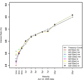
2.9 Yield Curve Estimation Comparison (14 Jun 2005) . . . 45
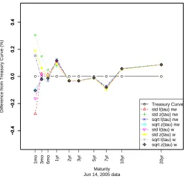
2.10 Yield Curve Estimation Difference Plot (14 Jun 2005) . . . 46
2.11 Yield Curve Estimation Comparison (28 Feb 2006) . . . 47
2.12 Yield Curve Estimation Difference Plot (28 Feb 2006) . . . 48
3.1 Discount Curve Bootstrap Results (14 Jun 2005) . . . 63
3.2 Discount Curve Bootstrap Results (28 Feb 2006) . . . 64
3.3 Caplet Pricing Bootstrap Means (outside knots) . . . 65
3.4 Caplet Pricing Bootstrap Coefficients of Variation (outside knots) . . . 66
3.5 Caplet Pricing Bootstrap Means (inside knots) . . . 67
3.6 Caplet Pricing Bootstrap Coefficients of Variation (inside knots) . . . . 68
3.7 Caplet Pricing Bootstrap Means (outside knots) . . . 69
3.10 Caplet Pricing Bootstrap Coefficients of Variation (inside knots) . . . . 72
3.11 Caplet Pricing Bootstrap Means (outside knots) . . . 73
3.12 Caplet Pricing Bootstrap Coefficients of Variation (outside knots) . . . 74
3.13 Caplet Pricing Bootstrap Means (outside knots) . . . 75
3.14 Caplet Pricing Bootstrap Coefficients of Variation (outside knots) . . . 76
Introduction
This chapter will provide background of the research areas involved in this dissertation
and a brief literature review of each. In Section 1.3, we discuss the Hull-White model for
short term interest rates as well as various aspects of the trinomial tree implementation
of this model used in this research. There is also a discussion of using the output of
the trinomial tree to price derivatives.
The remainder of this dissertation is arranged as follows. In Chapter 2, we describe
the bond data used in the subsequent analysis and discuss the procedure used to spline
the interest rate. There are also sections in this chapter related to the details of fitting
a spline to the interest rate term structure and a discussion of the treasury premium’s
relationship to using government bond prices to spline the risk-free interest rate. In
Chapter 3, we describe the methods used to bootstrap the trinomial tree pricing process
and present the results of the bootstrap analysis.
There are two appendices at the conclusion of this dissertation. Appendix A
pro-vides a detailed description of the construction of the trinomial trees used in this
research. Appendix B provides tables of results too lengthy to include in the main
1.1
Background
This section will cover background material in three different areas of research: a
history of interest rate models, an account of the role of smoothing spline methods in
our research, and a description of the statistical bootstrap.
1.1.1
Interest Rate Model Research
Research in the field of interest rate modeling is important for pricing interest rate
derivatives. An interest rate derivative is a financial instrument in which the payoff is
determined by a future level of a specified interest rate. Many types of interest rate
derivatives exist; the three most popular are bond options, interest rate swap options,
and interest rate caps/floors/collars. A bond option is an option where the underlying
asset is a bond. An interest rate swap option, or swaption, is an option to enter into
an interest rate swap where a specified interest rate is exchanged for a floating interest
rate.
An interest rate cap is a derivative that pays a notional amount multiplied by the
excess of a specified interest rate over the agreed-upon strike rate (also called the cap rate). The payment is structured as a stream of periodic payments, called caplets. The period length between payments is called the tenor of the agreement; generally, this length is three months (or a quarter of a year). An interest rate floor is similar to a
cap, except that it has a floor rate, which is a strike rate where the payoff depends on
the excess of the specified interest rate below the strike rate. An interest rate collar is
a derivative combining a cap and a floor to give protection against interest rates going
Terminology in the field of interest rate modeling differs greatly. In Yan (2001), the
author makes reference to the array of terminology:
The term structure of interest rates is also called “the yield curve of zero-coupon bonds.” With this correspondence in mind, I use “term structure” and “yield curve” interchangeably in this article. In market jargon, how-ever, the yield curve may refer to yields to maturity of on-the-run coupon bonds.
The development of the primary models in this field is covered thoroughly in the
literature review later in this introduction. Here we present a general roadmap of the
model types. The first models for the interest rate dealt with the short rate, which is
the annualized interest rate at which money can be borrowed for a very short time.
The first two classes of short rate models developed were equilibrium models and
no-arbitrage models. In an equilibrium model, the current term structure of the interest
rate is produced as an output of the model. In a no-arbitrage model, the current
term structure is an input of the model. Therefore, no-arbitrage models are able to
reproduce the current term structure exactly.
There are many models beyond the short rate models initially developed. The next
major set of models are called Heath-Jarrow-Morton (HJM) models. In an HJM model,
the instantaneous forward rate is modeled instead of the short rate. The most recent
developments in this field have been market models and infinite-dimensional models,
both of which are discussed in further detail in the literature review.
As an example of a short rate model to motivate the problem of modeling the
term structure of interest rates, we now present the Vasicek model in a general setting.
In the framework presented above, the Vasicek model is an equilibrium model. The
and mean reversion is incorporated into the model. This means that the process tends
to have negative drift when rates are high and positive drift when rates are low. This
corresponds to empirical results from the marketplace. Three constants, a, b, and
σ, in the model must be calibrated using the prices of financial instruments in the
marketplace. The model then uses the process dr = a(b−r)dt +σdz to model the
short rate r.1 The short rate r is pulled back towards the long-term mean b at a rate
of a, and a normally distributed stochastic term σdz is added to the mean reversion.
In this example, the instantaneous drift is a(b −r) and the instantaneous standard deviation isσ. This model is presented in detail in Hull (2003), who gives formulae for
pricing interest rate derivatives using the Vasicek model.
Further details of the progress of interest rate modeling are presented in
Sec-tion 1.2.1, and SecSec-tion 1.3 contains the technical details of the no-arbitrage class
Hull-White model for the short rate.
1.1.2
Spline Research
Spline methods were first introduced by I. J. Schoenberg (Schoenberg, 1946); in the
1960s and 1970s, a number of researchers including J. H. Ahlberg, Christian Reinsch,
and Grace Wahba built upon the ideas of Schoenberg. A brief review of the literature
as it relates to this research is included in Section 1.2.2. This section will give a brief
non-technical introduction to smoothing splines.
A spline allows a user to fit a smooth curve to a set of data. Spline methods come in
many variations, but the general concept consists of dividing the range of the data into
1
sections through the use of “knots”; a knot is a point that divides two such sections
of the data. Between knot points, a smooth curve is fit to the data, and conditions
are met so that the curves in each section of the data connect at each knot point.
Generally, derivative conditions must be met at the knot points to ensure smoothness
in the spline. The result is a smooth curve that fits the data according to a criterion
defined by the spline method itself.
Since this research involves cubic splines, we will briefly describe the procedure
for cubic spline construction. First, knot points are chosen; these can be chosen to be
equally spaced or not, according to the situation. (In this research, we choose the knots
points using a quantile approach so that the knot points are closer together where the
data is more dense and farther apart where the data is more sparse.) In each section of
the data between knot points, a cubic function is fit to the data. These cubic functions
must meet each other at the knot points such that their first and second derivatives
are continuous, ensuring a smooth spline function over the entire data set.
Historically, splines were developed outside of the mathematical arena. They were
first used by draftsmen and the aviation industry. The use by draftsmen is described
at the beginning of Ahlberg et al. (1967):
For many years, long, thin strips of wood or some other material have been used much like French curves by draftsmen to fair in a smooth curve between specified points. These strips or splines are anchored in place by attaching lead weights called “ducks” at points along a spline. By varying the points where the ducks are attached to the spline itself and the position of both the spline and the duck relative to the drafting surface, the spline can be made to pass through the specified points provided a sufficient number of ducks are used.
Finally, we mention the smoothing spline, which is a variation of a cubic spline in
that it adds a penalty term to the minimization criterion. This term penalizes excess
roughness (non-smoothness) in the spline fit. In general, the more knot points that
are used, the less smooth the fit will be. The use of smoothing splines allows the
user to use a large number of knot points and then smooth out the resulting fit as
needed. The method used to determine the value of the coefficient on the penalty term
is generalized cross validation (GCV). Generalized cross validation is a variation of
ordinary cross validation developed by Craven and Wahba (1979) for the case of spline
fitting. Ordinary cross validation for splines involved far too much computational time,
and GCV was able to shorten that time. More discussion of smoothing splines and
GCV is found in Section 1.2.2 and Chapter 2.
1.1.3
Bootstrap Research
The statistical bootstrap was introduced in 1979 by Bradley Efron. He introduced it
in light of the much older jackknife procedure, and detailed how the jackknife can be
thought of as a linear expansion method for approximating the bootstrap. The
statis-tical jackknife and statisstatis-tical bootstrap are resampling methods developed to estimate
the bias and standard error of a statistic. The jackknife was developed first. The
method of the jackknife is to successively remove one observation from a sample and
calculate the statistic of interest from this “jackknife sample.” There are n such
jack-knife samples in a sample of sizen observations. The jackknife bias and standard error
can then be computed using formulae provided in Chapter 11 of Efron and Tibshirani
In contrast to the jackknife, the statistical bootstrap resamples from a sample with
replacement. In the bootstrap world, the sample that has been collected is treated as
a substitute for the overall population, and another sample of the same size is taken
from the initial sample with replacement. This process is repeated many times, in
such a way that B independent bootstrap samples are taken, each consisting of n
observations selected with replacement from the initial sample ofn values. For each of
the B bootstrap samples, the statistic of interest is computed, and the standard error
is estimated by the sample standard deviation of the B replications. The bootstrap method allows estimation of standard errors with fewer distributional assumptions
being made regarding the data in question. Further details of the computations for the
single variable bootstrap will be provided in the beginning of Chapter 3.
The bootstrap has also been used for more complicated data structures than
univari-ate data. Chapters 8 and 9 in Efron and Tibshirani (1993) discuss the use of bootstrap
methods in two-sample problems, time series problems, and regression problems.
1.2
Literature Review
This section reviews the literature in interest rate modeling, spline methods, and
bootstrap methods. Two primary sources, the textbook Options, Futures, and Other Derivatives(Hull, 2003) and a Federal Reserve working paper entitled Fitting the term structure of interest rates with smoothing splines (Fisher et al., 1994), are briefly de-scribed in this introductory section. As in the Background section, the literature review
will be organized into three subsections corresponding to the three areas of research
Hull (2003) is a textbook designed for students and financial practitioners familiar
with finance and statistics concepts. Chapter 23 of Hull (2003) discusses numerous
models for the short rate, including the Hull-White model. A section in this chapter
describes the implementation of the trinomial tree that we used in the course of this
research.
Fisher et al. (1994) is a working paper published through the Federal Reserve that
describes a method to spline the term structure of interest rates using the market prices
of treasury bonds. We used this approach in our current research to provide an input
into the trinomial tree method for pricing interest rate derivatives.
1.2.1
Interest Rate Model Literature
Pricing models for interest rate derivatives date back to the 1980s when these
instru-ments were first developed in the marketplace. The earliest approach was to modify
the Black-Scholes (1973) model for pricing general options. However, Hull (2003)
men-tions that this model is appropriate when interest rates are assumed to be constant
or deterministic. Hull cites two questions that arise when interest rates are assumed
to be stochastic in this model: first, the Black-Scholes approach ignores that interest
rates are stochastic when discounting back to present value and second, this approach
ignores the fact that the forward price is not the same as the futures price. In light
of these concerns, Hull shows later that setting the futures price equal to the forward
price discounted at today’s T-year maturity zero rate is correct. This result shows that
this approach “therefore has a sounder theoretical basis and wider applicability than is
interest rates must be assumed to be stochastic because constant or deterministic
in-terest rates would make option pricing a trivial exercise.
For these reasons, a rich literature now suggests new models for the term structure
of interest rates. These include, in particular, two classes of “classic” models:
equi-librium models and no-arbitrage models. Both of these classes will be described in
this introduction. The most recent developments beyond these two classes of models
will also be reviewed. Special attention will be paid to the no-arbitrage class of term
structure models since it contains the Hull-White model, which is of primary focus in
this dissertation.
Equilibrium Models
The earliest departures from the Black-Scholes approach were the class of equilibrium
models, which use assumptions regarding economic variables to describe the evolution
of the zero curve through time. In one-factor equilibrium models, all the rates move in
the same direction, but not necessarily by the same amount (Hull, 2003). The
Rendle-man and Bartter model is the simplest one-factor equilibrium model. The process for
the short-term interest rate is modeled like a stock price using geometric Brownian
mo-tion without mean reversion (Rendleman and Bartter, 1980). Hull (2003) notes that
this is less than ideal since interest rates have historically reverted back to a long-term
mean. The Vasicek model, which incorporated mean reversion, addressed this concern.
However, this model had a downside as well since it allowed negative interest rates.
Although most research seems to agree that negative interest rates are inappropriate
in term structure models, Black (1995) has a brief discussion of this issue. Black notes
real interest rate may become negative, but the short rate cannot since individuals will
not keep their money in a negative interest-bearing instrument. They will instead put
their money in currency and receive an interest rate of zero percent.
The most popular of the one-factor equilibrium models is the Cox, Ingersoll, and
Ross model (denoted CIR model). Since it uses a square root process in the volatility
term, the model does not allow negative interest rates. This also implies that as interest
rates increase, the standard deviation of changes in the interest rate will increase as
well. The CIR model also incorporates mean-reversion like the Vasicek model (Hull,
2003). Of these three models, the CIR model has received the most attention in the
term structure modeling literature. However, the Vasicek model is the one that was
extended by Hull and White to develop the Hull-White model. Section 1.3 contains
more detailed explanations of the Hull-White model, including the formulae behind it.
Two-factor equilibrium models receive only a brief discussion in Hull (2003) and in
Hunt and Kennedy (2004). Hull (2003) mentions two models, Brennan-Schwartz and
Longstaff-Schwartz, that both have a second factor that allows for more flexibility in
modeling the term structure. Hunt and Kennedy (2004) note that two-factor models
are rarely used in derivative pricing primarily because of the difficulty in
implementa-tion.
No-arbitrage Models
An alternative approach to equilibrium models is the class of no-arbitrage models,
which contains the Ho-Lee and Hull-White models. Equilibrium models do not
nec-essarily match the current term structure, but no-arbitrage models are designed so
out-put of an equilibrium model, but it is an inout-put to a no-arbitrage model (Hull, 2003).
Ho and Lee (1986) presented the first no-arbitrage model. Their model was initially
described as a binomial tree of bond prices that included parameters to account for the
standard deviation of the short rate and for the market price of risk of the short rate.
Hull (2003) presents a continuous time limit of the discrete time process initially
pre-sented by Ho and Lee. In Hull and White (1990), the Vasicek model was extended so
that it took the current term structure as an input to the model. (Hunt and Kennedy
(2004) call the Hull-White model the Vasicek-Hull-White model since it is an extension
of the Vasicek model.) The Hull-White model also improved upon the Ho-Lee model
by incorporating mean-reversion, which the Ho-Lee model lacks. Both of these models
take the initial zero curve as an input, but neither model requires that the zero curve
be differentiable. Some no-arbitrage models can be implemented in a discrete-time
sense through the use of trees. Section 1.3.1 details the construction of a trinomial tree
in the case of the Hull-White model.
No-arbitrage models, like equilibrium models, began with only one function of time,
but by making a second parameter also a function of time, no-arbitrage models can
be more closely fitted to current market data of actively traded options. Hull (2003)
briefly discuss two such extensions, the Black-Derman-Toy binomial tree procedure and
the Black-Karasinski model. The downside to these models is that they can produce
future volatility term structures that are quite different from the current volatility term
structure.
All of these models also involve calibration to determine the values of their
ters. Hull (2003) gives a general description of the calibration procedure. The
measure such as minimizing the sum of squared differences between the market price
and the model price of each instrument being used for calibration.
Pricing interest rate derivatives using the interest rate models discussed thus far
has two main limitations. First, they only have one source of uncertainty. Second,
they do not offer complete freedom in choosing the volatility structure. More recent
efforts have addressed these issues by including a second factor (source of uncertainty).
These efforts include models developed by Duffie and Kan (1994) and Hull and White
(1994). The two-factor Hull-White model still matches the initial term structure
ex-actly, but since it has a second source of uncertainty, it allows for more variation in
the term structure to better capture the differing amounts of volatility in the forward
rate throughout the term to maturity.
More Recent Models
Another approach to modeling the yield curve involves modeling the processes that are
followed by instantaneous forward rates. The primary model in this approach is the
Heath-Jarrow-Morton (HJM) model. The HJM model is a generalization of the
Ho-Lee model to multiple factors over continuous time. The HJM model takes the initial
forward rate curve as given and describes its evolution across time using a continuous
time stochastic process (Heath et al., 1992).
Hull (2003) notes that one negative aspect of the HJM model framework is the
difficulty of calibrating the model to the prices of actively traded instruments. Yan
(2001) also points out that since HJM models use continuous compounding of the
instantaneous forward rate curve, specifying a lognormal process in the HJM framework
models has been on two fronts: LIBOR (London Interbank Offered Rate) or market
models and so-called “infinite-dimensional” models. Yan (2001) claims that the market
models enjoy the most widespread use in the financial industry.
Market models deal directly with observable rates in the marketplace, and they give
the user complete freedom in specifying the term structure of the volatility. Brace et al.
(1997), Jamshidian (1997), and Miltersen et al. (1997) all developed models of the
for-ward rate that are used by traders in practice. Miltersen et al. (1997) present a model
that provides closed form solutions for interest rate derivative prices that coincide with
results obtained from a modified Black-Scholes formula. They also show that by
spec-ifying a particular volatility structure, the lognormal assumption on forward rates is
consistent with the HJM model. Hull (2003) points out that both HJM and LIBOR
models have the disadvantage of not being easily implemented using recombining trees;
instead, Monte Carlo simulation must be used to implement these models.
(Recom-bining trees are binomial or trinomial trees where the paths taken by going down and
then up or up and then down lead to the same node. Recombining trinomial trees have
2n+ 1 nodes at timestepn, whereas non-recombining trinomial trees have 3n nodes at timestep n.)
The final area of interest rate models is the class of “infinite-dimensional” models;
this area also goes by the terms “random-field” or “stochastic-string” models (Yan,
2001). In recent years, a number of developments in this area have been presented.
In Sornette (1998), the term structure is formulated in such a way that the forward
curve is viewed as the deformation of a “string.” The article details the analogy of the
forward curve in terms of string theory in physics. Goldstein (2000) uses random fields
since it does not require recalibration, it provides a parsimonious description of term
structure dynamics, and it naturally accounts for the fact that the best hedge for a
bond is one of a similar maturity. Goldstein also points out that random field models
of the term structure are generalizations of finite-factor models, but they are consistent
with the current yield curve and term structure innovation. Yan (2001) recognizes that
infinite-dimensional models provide straightforward pricing of bond options. Finally,
Izzi and Racheva (2002) present a new model based on the assumption that the short
rate follows a mean-reverting jump-diffusion process that is the sum of one Brownian
motion and a finite number of Poisson processes. However, this model requires the
development of a recombining hexanomial tree that fits the current term structure
observed in the market.
1.2.2
Spline Literature
As mentioned in Section 1.1.2, the mathematical spline was adapted from industrial
practice by I. J. Schoenberg (Schoenberg, 1946) and developed further in the 1960s
and 1970s. This section will describe a few of the developments at that time in terms
of smoothing splines and generalized cross validation (GCV). The literature review
presented here will be restricted to the part of spline research used in this dissertation,
specifically the use of smoothing splines to estimate the zero curve.
In 1964, Schoenberg combined the work done thus far on spline interpolation and the
problem of graduation of data discussed by E. T. Whittaker (Whittaker and Robinson,
1926). (Whittaker had introduced the problem of graduation, which was a precursor
Whittaker and Robinson (1926).) Schoenberg used one of these methods in relation to
spline functions; this led to the introduction of a criterion for evaluating the goodness
of fit of a spline curve to data. This two part minimization criterion problem laid the
ground work for the GCV work in subsequent research. Essentially, the first part of the
minimization problem measures the distance of the spline curve from the data points
and the second part measures the smoothness of the spline curve.
Reinsch (1967) modified the approach of Schoenberg to replace interpolation of the
data with an algorithm for smoothing experimental data. In this article as well as
Reinsch (1971), Reinsch cites a result from Schoenberg (1964) that states that the
unique solution to the two part minimization problem described above is a natural
spline of degree 2m−1 wherem is less than or equal to the number of knot points.
The problem that arose from the work to this point, however, was the tradeoff
between the two parts of the minimization problem. In the general problem, a single
parameter (λ) coefficient on the second part of the problem measured the roughness
of the spline curve. Since this parameter somehow had to be chosen, the choice of this
parameter was the focus of much work. Reinsch (1967) presents an interval (dependent
upon σ2) within which to choose the roughness parameter. (Here, σ2 is the variance
of the error terms between the observed data points and the true but unknown curve.)
Wahba (1975) suggests choosing the roughness parameter to be less thanσ2by a “fudge
factor”; this approach allows the author to determine an optimal λ value when σ2 is
known.
Since σ2 is not generally a known value, Craven and Wahba (1979) developed an
optimal method of smoothing that did not require knowledge of σ2. This method,
that allows for faster computation, an important consideration at a time when
com-putational time was more critical than today. Further details of the GCV calculations
are included in Chapter 2.
Fisher et al. (1994) utilize the GCV formulation for smoothing splines to estimate
the yield curve from bond data. The entire formulation is summarized in Wahba
(1990). Fisher et al. (1994) use the GCV method to choose an appropriate value of λ.
They cite that the advantage to such an approach is that “the shape of the spline is
controlled by a single parameter.” Chapter 2 also contains further details of the use of
GCV in the estimation of the yield curve.
1.2.3
Bootstrap Literature
As mentioned in Section 1.1.3, the concept of the statistical bootstrap was introduced
by Bradley Efron (Efron, 1979). Since then, the bootstrap methodology has been used
in a variety of situations. This section will focus on the part of the literature dealing
with regression problems. The basic bootstrap methodology deals with univariate
in-dependent and identically distributed samples, but in the case of regression problems,
the data are no longer univariate and generally correlation exists between the
indepen-dent variables. Therefore, the basic bootstrap has been extended to handle regression
problems.
Extensions to the initial bootstrap methodology appeared soon after Efron’s
orig-inal article. For instance, Bickel and Freedman (1981) provide asymptotic theory to
show that the bootstrap introduced by Efron is valid in a large number of situations,
distribution. The first work to extend the bootstrap to regression problems was
pub-lished two years after Efron’s introduction of the bootstrap. Freedman (1981) examines
a bootstrap approach for estimating the distribution of linear least squares estimates.
The regression bootstrap resamples from the bootstrap centered residuals. The
cen-tered residuals are calculated by subtracting the mean of the residuals from each of
the residuals, which are the differences of the observed value minus the predicted value
of the dependent variable. This approach relies on the residuals obtained from the
initial regression model to determine the bootstrap samples. The author notes that
the bootstrap will generally fail if the residuals are not centered prior to performing
the resampling procedure. This article also includes details for bootstrapping in the
multiple linear regression case.
Efron and Gong (1983) provide a simple explanation of the bootstrap procedure and
include an example of using the bootstrap to estimate the correlation coefficient in the
simple linear regression setting. They claim that “it can be applied just as well to any
statistic, simple or complicated, as to the correlation coefficient.” Bickel and Freedman
(1983) consider the bootstrap for a regression model where both the number of data
points and the number of parameters are both large. Their results focus on the ratio
of the number of parameters to the number of data points; if this ratio is small, the
bootstrap approximation to the distribution of contrasts is valid. They also show that
if this ratio does not tend to zero, the bootstrap approximation is not valid.
The first application of the bootstrap to generalized least squares appeared one year
later (Freedman and Peters, 1984); the authors describe the bootstrap as a “technique
for estimating standard errors,” and apply the bootstrap in the context of an
for energy. They emphasize that the initial regression model must be valid in order
for residual-based bootstrap techniques to work. This concern is also voiced by Weber
(1985), where two different methods of regression bootstrapping are compared. The
first method, the one discussed in the literature up to this point, relies heavily on the
regression model by resampling from the residuals to reconstruct dependent variable
values in the bootstrap samples. The author notes that this approach is susceptible to
model misspecification since the bootstrap samples rely upon the model being correctly
specified. The second approach, which Weber favors, is to resample with replacement
directly from the original data points to create bootstrap samples. He states that
this approach is robust against heterogeneity of the error variance, noting that despite
Efron and Gong (1983) mentioning this observation in passing, it is not emphasized in
the bootstrap literature. This second approach is also easier to implement than the
residual bootstrap.
Shao (1988) shows that the bootstrap method implemented by resampling residuals,
the first method described in the previous paragraph, is asymptotically correct only
in the case of a homoskedastic error model. This article also finds that bootstrapping
residuals in the heteroskedastic case results in the variance estimator having a larger
mean square error than in the jackknife estimator.
Finally, Efron and Tibshirani (1993, Chapter 9) weigh in again to discuss the
two different approaches to the regression bootstrap first compared by Weber (1985).
Efron and Tibshirani call these approaches “bootstrapping residuals” and
ping pairs,” and they prefer bootstrapping pairs. However, they note that
“bootstrap-ping is not a uniquely defined concept.” They also include examples of using the
1.3
Hull-White Yield Curve Model
In this section, various aspects of the Hull-White model for short term interest rates are
discussed. Section 1.3.1 presents the model and a brief description of the trinomial tree
discretization of the model. (Appendix A contains a full description of the trinomial
tree construction used in this research.) Section 1.3.2 presents an example of pricing
an interest rate derivative using the trinomial tree.
Before describing the Hull-White model in detail, we take a moment to put the
model in context of the history of interest rate models. Much of this history is covered
in Section 1.2.1. The reader is reminded of four classes of interest rate models:
equi-librium, no-arbitrage, market (or LIBOR), and infinite-dimensional. The first type of
models developed were equilibrium models, but these models did not match the initial
term structure of interest rates exactly and led to mispricing of bonds and more severe
mispricing of options. (Hull (2003) notes that a 25% error in option pricing can result
from as little as a 1% error in in the pricing of the underlying bond.) For this reason,
no-arbitrage models were developed; these models use the current term structure of
interest rates as an input and are then able to match today’s term structure exactly.
The Hull-White model belongs to the no-arbitrage class of models.
More recent developments in interest rate modeling are related in the literature
re-view. In general, the models have become more complex as computing power increases
1.3.1
Model Description and Discretization
The Hull-White model (Hull, 2003, page 546) is a model for the short rate that provides
an exact fit to the initial term structure. The short rate (or short-term risk-free rate)
is the interest rate applicable for a very short period of time. The term structure
of interest rates is the relationship between interest rates and their maturities. The
Hull-White model is specified as follows:
dr = [θ(t)−ar]dt+σdz (1.1)
where r is the short rate, z is a Wiener process, and a and σ are constants. A Wiener process is a Brownian motion; it has mean change of zero, a variance rate of one
(per year), and the values of its changes for any two different short time intervals are
independent (Hull, 2003). The function θ(t) is then calculated from the initial term
structure:
θ(t) = Ft(0, t) +aF(0, t) + σ2
2a 1−e
−2at
(1.2)
where F(0, t) is the instantaneous forward rate for a maturity t at time zero. The
subscript t denotes the partial derivative with respect to t. Hull notes that the third
term of θ(t) is often small. Therefore, the majority of the drift of r is represented by
Ft(0, t) +a(F(0, t)−r), which is the slope of the instantaneous forward rate curve plus
a term that causes r to revert back to that curve at a rate of a.
In the current research, a and σ are fixed constants. Further study is required to
determine the effects of variability of estimates for a and σ on the eventual pricing of
Hunt and Kennedy (2004, Chapter 17) praise the Hull-White model for its
tractabil-ity, stating that this is important so that the model can be efficiently calibrated to
market prices. The authors show that the solution to the Hull-White stochastic
dif-ferential equation is a Gaussian process, which allows users to calibrate the model to
bond and option prices. Also, the distribution of the short rate rt (given rs, where
t ≥s) is Gaussian.
The Hull-White model is a continuous-time model. However, in the current analysis,
a discrete-time approximation will be used. The implementation of the Hull-White
model that will be used in this analysis is through the use of a recombining trinomial
tree (Hull, 2003, page 552). A trinomial tree starts at time zero with one node and has
three branches that extend to the right (one timestep into the future) to three nodes.
From each of those three nodes, three more branches extend to nodes at the next
timestep for a total of five nodes. In this work, we use recombining trees, meaning that
branches recombine from one timestep to another. (For an example of a recombining
trinomial tree, see Figure 1.1.) Hence, the total number of nodes at a given timestep is
less than if this recombining did not take place. Indeed, a non-recombining trinomial
tree has 3n nodes at timestepn, whereas a recombining trinomial tree has only 2n+ 1
nodes at timestepn. The tree terminates on the horizontal (time) axis at a time called
maturity. In this analysis, the timesteps are all the same length, and the amount
of increase or decrease at each branch is initially the same. Hull (2003) notes that
trinomial trees (rather than binomial trees) are preferred for interest rate trees since
trinomial trees offer an extra degree of freedom which allows them to better match
the mean reversion property of some interest rate models. See Appendix A for a more
A value for the zero curve is required at every timestep of the tree. For this reason,
we use a spline approximation to the zero curve in Chapter 2. Also, in order to obtain
values for the interest rate at each node at the final timestep of the tree, the value of
the zero curve at one timestep past the final timestep of the tree is required.
1.3.2
Pricing Derivatives Using the Trinomial Tree
The trinomial trees constructed in this research can be used to price securities based
on interest rates, including zero coupon bonds and interest rate derivatives, such as
interest rate caplets. Caplets are the individual payments that make up the stream
of payments comprising an interest rate cap. Interest rate caps are described in some
detail in Section 1.1.1, but we will introduce them again here and go through a simple
example of using a trinomial tree to price a caplet.
An interest rate cap is a financial derivative that uses a specified interest rate level
as the underlying asset on which the payoff of the cap is determined. In this framework,
a cap rate is compared to the floating rate at each of the specified payoff times. If the
floating rate is above the cap rate, there is a payoff; otherwise, no payoff occurs at that
time. These times are generally spaced quarterly throughout the year (once every three
months), and this period of time is called the tenor of the cap agreement. Each payoff
in the cap is called a caplet. If a payoff occurs, it is determined by multiplying the
excess of the floating rate over the cap rate by the notional amount (specified as part of
the cap agreement). An interest rate cap therefore provides the holder with insurance
against rising interest rates, since the payoffs help offset other negative effects of rising
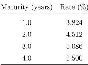
Table 1.1: Zero Rates Used in Pricing Example
Maturity (years) Rate (%)
1.0 3.824
2.0 4.512
3.0 5.086
4.0 5.500
We will now illustrate the use of the trinomial tree to price a caplet. The example
tree is a modified version of the tree used in Hull (2003) as an illustration of constructing
a trinomial tree. The zero rates used in this example are listed in Table 1.1. The
caplet in this example will have a cap rate of 8%, a notional amount of $10,000,000,
and quarterly reset (payoff) dates. Thus, the tenor is three months. The caplet we are
pricing is three years into the future. The trinomial tree will use the zero rates given
in Table 1.1 and one timestep per year.
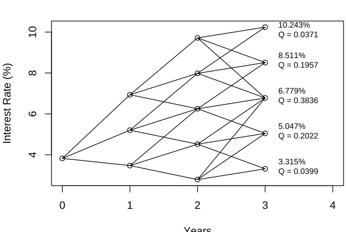
The resulting trinomial tree shown in Figure 1.1 is then used to price the caplet.
Each node at the end of the tree is labeled with an interest rate (top line) and a Q
value (bottom line). The interest rate value is the level of the interest rate at that
particular node. The Q value for a particular node is the present value of a security that pays $1 if that node is reached and pays nothing otherwise. (For more details on
the construction of the trinomial tree and the calculation of the values in the tree, see
Appendix A.)
Since the cap rate in this example is 8%, the only nodes that contribute to the
0 1 2 3 4
4
6
8
10
Trinomial Tree Illustration
Years
Interest Rate (%)
10.243% Q = 0.0371 8.511% Q = 0.1957
6.779% Q = 0.3836
5.047% Q = 0.2022
3.315% Q = 0.0399
Figure 1.1: Trinomial Tree Illustration
rates throughout are expressed as annual rates, so for a quarterly reset date, the rates
must be multiplied by 0.25. For each node above the cap rate, the excess of the node’s
interest rate over the cap rate is multiplied by theQvalue of the node. Then, the price
of the caplet is:
0.25∗[(0.10243−0.08)∗0.0371 + (0.08511−0.08)∗0.1957]∗$10,000,000 = $4,580.45
This example shows how the trinomial tree described in Section 1.3.1 can be used
interest rate andQ for the final timestep. However, more complicated derivatives that are path-dependent may require calculations using values from nodes other than the
nodes at the final timestep. In cases such as these, the tree construction is the same,
but the values at nodes prior to the end of the tree must either be stored or used during
the tree construction to determine the price of the derivative.
Another case mentioned at the beginning of this section is zero coupon bond pricing.
The present value of a zero coupon bond maturing in three years in this example would
be De−3(.05086) = 0.85849D, where D is a notional amount for the bond; this result
follows from the zero curve value at three years maturity being 5.086%. This value can
also be derived from the Q values on the trinomial tree. Summing theQ values at the
three year mark gives the value 0.8585, which is the same value as the present value
of the three year zero coupon bond. This result holds because the Q values represent
the present value of a security that pays $1 if a particular node is reached. For a zero
coupon bond, however, it does not matter which node is reached at maturity; the bond
will pay off its face value. Therefore the present value of the bond is the sum of the
Modeling the Term Structure
The trinomial tree algorithm of Section 1.3 requires a value of the zero curve at every
timestep. Therefore, to explore the effects on pricing of decreasing the intervals
be-tween timesteps, we need to model the term structure of the zero curve such that it
can be evaluated at every timestep. For this purpose, we adapt and expand upon a
spline method proposed for the term structure of interest rates by Fisher et al. (1994).
The method involves the use of smoothing splines with a cubic B-spline basis. We
instead use smoothing splines with a natural spline basis; this choice is explained
fur-ther in Section 2.2. The smoothing spline is based on a regression spline and is then
smoothed through the use of a smoothing parameter λ. This approach, recommended
by Fisher et al., uses a large number of knot points and penalizes excess variability
us-ing the smoothus-ing parameter. To choose λ, we minimize a generalized cross validation (GCV) value over a grid search for the optimalλ. We further explore extensions to the
Fisher et al. (1994) method by comparing different timescales and adding a weighting
scheme to the data to account for unequal amounts of variability at the short and long
term maturities. We also extend their method to spline the zero curve directly; see
Section 2.8.2 for a more detailed explanation of this extension.
The remainder of this chapter describes the process of modeling the term structure.
reports an analysis comparing the cubic B-spline basis and the natural spline basis,
and Sections 2.3 through 2.5 describe the results of the various adaptations to the
Fisher et al. (1994) method. Section 2.5 compares our spline results to those of the
US Treasury Department and also summarizes the comparisons between the many
variations of the spline process. In Section 2.6, we include a brief discussion of the
treasury premium as this topic relates to our research. Section 2.7 describes a spline
method to bypass the spline for the zero curve. Finally, Section 2.8 contains background
calculations for the chapter.
2.1
Description of the Data and Notation
The treasury security price data we use to model the term structure of the interest
rate was obtained from the 15 June 2005 Wall Street Journal (2005) and the 1 March 2006 Wall Street Journal(2006); we refer to these two data sets as the June 2005 data set and the February 2006 data set. All treasury bills and notes were used. Treasury
bonds were also used, with the exception of inflation-indexed issues and callable bonds
(denoted in USGAO (1999)). This follows the guidelines set forth by Fisher et al.
(1994). The maturity dates were obtained from the Treasury department website1.
These dates were used to determine the amount of accrued interest to add to the
quoted price for interest-bearing bonds and notes. (Bills are zero-coupon instruments,
and therefore they have no accrued interest.)
The calculation of accrued interest was performed according to Fabozzi (1997); the
semiannual coupon payment was multiplied by the accumulated time since the last
1
coupon payment (measured as the number of days since the last payment divided by
the number of days in the current coupon payment period). This accrued interest
amount was then added to the security’s quoted price.
We use the notationδ(τ) to refer to the discount function of a one unit zero coupon
bond maturing at time τ. We define l(τ) = −log(δ(τ)), and the zero curve z(τ) =
l(τ)/τ. We also denote the natural spline basis functions with the notationφ and the
coefficients on those basis functions β.
2.2
Comparison of Two Cubic Spline Bases
Fisher et al. (1994) advocate the use of a cubic B-spline basis to spline the zero curve.
In our research, we have opted to use a natural cubic spline instead. This section
reports the results of a comparison of the two methods.
For the ith bond, the quoted market price is denoted P
i, and πi is the predicted
price. Degrees of freedom are determined by the number of interior knots used in the
spline procedure. A cubic B-spline basis has degrees of freedom equal to the number
of interior knots plus four; a natural cubic spline basis has degrees of freedom equal to
the number of interior knots plus two2. The error degrees of freedom is calculated as
the difference between the number of data points (N) and the degrees of freedom for
the spline fit. The mean squared error (MSE) is calculated by dividing the error sum of
squares (SSE) by the error degrees of freedom. We conclude that there is no significant
effect of using a natural cubic spline basis rather than a cubic B-spline basis. For the
2
Table 2.1: Spline Comparison (14 Jun 2005)
Natural Spline B-spline
N (# of bonds used in spline) 160 160 Mean (Pi−πi) 0.00245 0.00245
StdDev (Pi−πi) 0.08317 0.08296
Degrees of Freedom (fit) 53 55
Degrees of Freedom (error) 107 105 SSE =P
(Pi−πi)2 1.10071 1.09532
MSE = df1 P
(Pi−πi)2 0.01029 0.01043
Table 2.2: Spline Comparison (28 Feb 2006)
Natural Spline B-spline
N (# of bonds used in spline) 169 169 Mean (Pi−πi) 0.00023 0.00026
StdDev (Pi−πi) 0.20973 0.20524
Degrees of Freedom (fit) 56 58 Degrees of Freedom (error) 113 111
SSE =P
(Pi−πi)2 7.39011 7.07684
MSE = df1 P
(Pi−πi)2 0.06540 0.06376
2.3
Effects of Changing the Timescale
We explore the effects of changing the timescale in the spline process for the interest
rate term structure. Initially, the timescale of the bond data input into the spline
procedure was on a standard linear timescale. In this section, the standard timescale
approach is compared to a square root timescale approach.
Before presenting the results of this section, we provide some details of the
com-putations involved in changing the timescale in the spline procedure. In the
stan-dard spline procedure proposed by Fisher et al., the spline is created for l(τ), where
l(τ) = −log(δ(τ)) = τ z(τ). (Here, δ(τ) is the discount function with a current time
of zero and z(τ) is the zero curve.) We spline l(τ) and then convert the spline to be a
representation of the zero curve.
To illustrate changing the timescale that is input into the spline procedure, we will
briefly discuss the process for the square root timescale. First, the maturities and times
to payoff dates for the bond data are replaced by their respective square root values.
Next, we modify the calculation of the penalty term in the spline procedure to use a
natural spline basis calculated on a fine grid over maturities of 0 to √30 rather than
0 to 30 as in the standard timescale. In the standard timescale, l(t) = φβ and the
zero curve is a plot of z(t) =φβ/t against√t. In the square root timescale, l(t) =φβ
(calculated with the square root maturities and times to payoffs) and the zero curve is
a plot of z(t) =φβ/t against√t. As shown in the remainder of this section, the square
root approach allows for greater flexibility in the spline fit for short term maturities
and a more rigid fit for long term maturities.
0.0
0.6
1.2
Maturity
Spline, l(t)
1mo 3mo 6mo 1yr 2yr 3yr 5yr 7yr 10yr 20yr
2.5
3.5
4.5
Maturity
Zero Curve (%)
1mo 3mo 6mo 1yr 2yr 3yr 5yr 7yr 10yr 20yr
−0.2
0.2
Standard Timescale, June 2005 Data Maturity
Residuals ($)
1mo 3mo 6mo 1yr 2yr 3yr 5yr 7yr 10yr 20yr
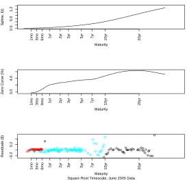
Figure 2.1: Standard Timescale (14 Jun 2005)
root timescales for the June 2005 bond data set, as well as a comparison of the residuals
obtained using each timescale. Analogous results are also presented for the February
2006 data set.
June 2005 Data Set Results
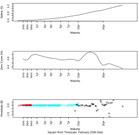
In Figure 2.1, the top panel shows the spline for l(τ) using the bond data with a
standard linear timescale. The second panel shows the zero curvez(τ), which is derived
from l(τ) using the relationshipz(t) = l(t)/t. The third panel displays the residuals,
0.0
0.6
1.2
Maturity
Spline, l(t)
1mo 3mo 6mo 1yr 2yr 3yr 5yr 7yr 10yr 20yr
3.0
4.0
Maturity
Zero Curve (%)
1mo 3mo 6mo 1yr 2yr 3yr 5yr 7yr 10yr 20yr
−0.2
0.2
Square Root Timescale, June 2005 Data Maturity
Residuals ($)
1mo 3mo 6mo 1yr 2yr 3yr 5yr 7yr 10yr 20yr
Figure 2.2: Square Root Timescale (14 Jun 2005)
predicted price of bond i based on the spline procedure. The colors of the residuals in
the third panel of the plots in this chapter refer to the type of Treasury security the
residual refers to: red refers to Treasury bills (maturity of one year or less), blue refers
to Treasury notes (maturity of two to ten years), and black refers to Treasury bonds
(maturity of ten years or longer). All three panels are plotted with a horizontal axis
of time on a square root scale.
The results for the square root timescale are shown in Figure 2.2. The three panels
correspond to the three panels from the figure for the standard timescale approach.
2.5
3.0
3.5
4.0
4.5
5.0
Maturity
Zero Curve (%)
1mo 3mo 6mo 1yr 2yr 3yr 5yr 7yr 10yr 20yr
2.5
3.0
3.5
4.0
4.5
5.0
Maturity
Zero Curve (%)
Standard Timescale Square Root Timescale
Figure 2.3: Zero Curve Comparison (14 Jun 2005)
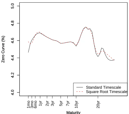
the zero curves produced by each approach are shown in Figure 2.3. The solid line is
the zero curve obtained from using a standard timescale, and the dashed line is the
zero curve obtained from using a square root timescale. The square root timescale zero
curve exhibits more flexibility at the short term maturities (specifically maturities less
than 2 years), but the standard timescale zero curve exhibits more flexibility at the
long term maturities (roughly 20 years or more). The curves presented in Figures 2.1
through 2.3 were plotted by calculating the zero curve value monthly from 0 to 12
months and then annually from 1 to 30 years.
Table 2.3: SSE Comparison (14 Jun 2005)
Bin n Standard timescale Square root timescale
Overall 160 1.1007 1.3896
0-1 years 47 0.1620 0.1372
1-4 years 45 0.0371 0.0365
4-9 years 26 0.2978 0.3776
9-16 years 21 0.3792 0.4043
≥16 years 21 0.2247 0.4339
sums of squared residual terms both overall (for all maturities) and in five different
bins based on maturities. (The sum of squared residuals (SSE) is P
(Pi−πi)2, where
the ith quoted market price is denoted P
i and πi is the ith predicted price.) These
comparisons are shown in Table 2.3. The SSE for the square root timescale is greater
when computed for all 160 bonds in the 14 Jun 2005 data set; however, for the short
term maturity bins ([0,1] and (1,4]), the square root timescale approach has smaller
sums of squared residuals. This again shows that the square root timescale is fitting
the bond data set prices more closely (i.e. with more flexibility in the spline process)
for the short maturities. Conversely, the SSE values for the standard timescale are
smaller than for the square root timescale at long term maturity values (greater than
4 years). Table 2.4 reports the means and standard deviations of the residuals both
Table 2.4: Mean and Standard Deviation Comparison (14 Jun 2005)
Bin n Standard timescale Square root timescale
Overall 160 0.0024 (0.0832) 0.0023 (0.0935) 0-1 years 47 0.0021 (0.0593) -0.0001 (0.0546) 1-4 years 45 0.0022 (0.0290) 0.0048 (0.0284) 4-9 years 26 0.0001 (0.1091) -0.0007 (0.1229)
9-16 years 21 0.0086 (0.1374) 0.0075 (0.1420)
≥16 years 21 0.0006 (0.1060) 0.0011 (0.1473)
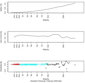
February 2006 Data Set Results
Analogous results are now presented for the February 2006 bond data. Figures 2.4
and 2.5 display the results of the spline process for the standard and square root
timescales, respectively. Figure 2.6 shows the comparison plot for the 28 February
2006 data. Once again, the square root timescale curve shows more flexibility in the
first year of maturity and less flexibility at longer maturities, especially those over 16
years. Table 2.5 shows the SSE values for the overall curves as well as for the bins of
maturities used in the previous tables of this section. Once again, the overall SSE for
the square root timescale is greater than the overall SSE for the standard timescale.
However, in the first two bins (up to 1 year and 1 to 4 years), the SSE for the square
root timescale is less than the SSE for the standard timescale. In Table 2.6, the means
and standard deviations of the residuals are reported for the overall residuals and for
0.0
0.6
1.2
Maturity
Spline, l(t)
1mo 3mo 6mo 1yr 2yr 3yr 5yr 7yr 10yr 20yr
4.0
4.4
4.8
Maturity
Zero Curve (%)
1mo 3mo 6mo 1yr 2yr 3yr 5yr 7yr 10yr 20yr
−1.5
0.0
Standard Timescale, February 2006 Data Maturity
Residuals ($)
1mo 3mo 6mo 1yr 2yr 3yr 5yr 7yr 10yr 20yr
Figure 2.4: Standard Timescale (28 Feb 2006)
Table 2.5: SSE Comparison (28 Feb 2006)
Bin n Standard timescale Square root timescale
Overall 169 7.3901 9.8405
0-1 years 49 0.0298 0.0280
1-4 years 51 0.0412 0.0390
4-9 years 27 0.7812 0.8264
9-16 years 22 0.2450 0.3702
0.0
0.6
1.2
Maturity
Spline, l(t)
1mo 3mo 6mo 1yr 2yr 3yr 5yr 7yr 10yr 20yr
4.4
4.6
Maturity
Zero Curve (%)
1mo 3mo 6mo 1yr 2yr 3yr 5yr 7yr 10yr 20yr
−1.5
0.0
Square Root Timescale, February 2006 Data Maturity
Residuals ($)
1mo 3mo 6mo 1yr 2yr 3yr 5yr 7yr 10yr 20yr
Figure 2.5: Square Root Timescale (28 Feb 2006)
Table 2.6: Mean and Standard Deviation Comparison (28 Feb 2006)
Bin n Standard timescale Square root timescale
Overall 169 0.0002 (0.2097) -0.0005 (0.2420) 0-1 years 49 -0.0009 (0.0249) -0.0006 (0.0241) 1-4 years 51 0.0027 (0.0286) 0.0022 (0.0278) 4-9 years 27 -0.0094 (0.1731) -0.0148 (0.1776)
9-16 years 22 0.0276 (0.1043) 0.0452 (0.1244)
4.0
4.2
4.4
4.6
4.8
5.0
Maturity
Zero Curve (%)
1mo 3mo 6mo 1yr 2yr 3yr 5yr 7yr 10yr 20yr
4.0
4.2
4.4
4.6
4.8
5.0
Maturity
Zero Curve (%)
Standard Timescale Square Root Timescale
Figure 2.6: Zero Curve Comparison (28 Feb 2006)
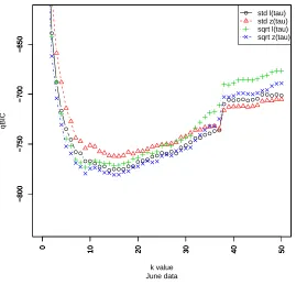
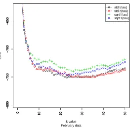
2.4
Incorporating Weights into the Spline Fit
This section details the formulation of the criterion for determining the optimal
smooth-ing parameter in the weighted case of the Fisher et al. (1994) (FNZ) zero curve spline
analogous to the generalized cross-validation (GCV) criterion. The section will describe
the reasoning behind adding weights to the market bond data and our adaptation for
weighted data to the Craven and Wahba (1979) approach. The attempt to incorporate
some type of weighting into the FNZ zero curve spline analysis was driven by the
FNZ predicted bond prices π), as seen in the third panel of Figure 2.1. The residuals are small in the short term of maturities, but they increase at longer maturities.
Our solution is to incorporate a weight matrixW into the FNZ algorithm. The W
matrix is annxndiagonal matrix constructed element by element using ak-th nearest
neighbor variance estimation algorithm, where n is the number of observations in the
data set and k is the number of nearest neighbors included in the calculation. For
example, the first element, corresponding to the first observation, finds the k nearest
residuals on the maturity (horizontal) axis and averages the sum of those squared
residuals. This is an estimate of the variance of the first observation’s residual (s2
i),
defined in Equation 2.3 (page 42). The W matrix is constructed by inverting these
variance estimates, such that wi = 1/s2i and W = diag(w1/w, w2/w, ..., wn/w), where
w is the mean of the wi values. Hence, W is a diagonal weight matrix standardized
such that the diagonal elements have a mean of one.
Next, we refer back to the original GCV paper by Craven and Wahba (1979). The
remainder of this section details the adaptation of their method of GCV calculation
to find an analogous version of the GCV for the weighted data case. (The following
description refers to Craven and Wahba (1979); we use the notation (CW 1.1) to refer
to their Equation 1.1.) The authors start with a mathematical model:
y(t) = g(t) +ǫ(t), t ∈[0,1] (CW 1.1)
where g(t) is a “smooth” curve, ǫ(t) is a white noise process, and y(t) is the observed
where:
W