A study on component-based technology for development of complex bioinformatics software

(1)

75031

A STUDY ON COMPONENT-BASED TECHNOLOGY FOR

DEVELOPMENT OF COMPLEX BIOINFORMATICS SOFTWARE

ZURAINI ALI SHAH

SAFAAI DERIS

MUHAMAD RAZIB OTHMAN

ZALMIYAH ZAKARIA

PUTEH SAAD

ROHAYANTI HASSAN

MOHD HILMI MUDA

SHAHREEN KASIM

ROSFUZAH ROSLAN

FACULTY OF COMPUTER SCIENCE AND INFORMATION SYSTEMS

UNIVERSITI TEKNOLOGI MALAYSIA

(2)

ABSTRACT

In the first chapter, entitled “Enhancement of Support Vector Machines for Remote Protein

Homology Detection and Fold Recognition,” M. Hilmi Muda, Puteh Saad and Razib M. Othman

present a comprehensive method based on two-layer multiclass classifiers. The first layer is used

to detect up to superfamily and family in SCOP hierarchy, by using optimized binary SVM

classification rules directly to ROC-Area. The second layer uses discriminative SVM algorithm

with a state-of-the-art string kernel based on PSI-BLAST profiles that is used to leverage the

unlabeled data. It will detect up to fold in SCOP hierarchy. They evaluated the results obtained

using mean ROC and mean MRFP. Experimental results show that their approaches significantly

improve the performance of protein remote protein homology detection for all three different

datasets (SCOP 1.53, 1.67 and 1.73). They

achieved 0.03% improvement in term of mean ROC

in dataset SCOP 1.53, 1.17% in dataset SCOP 1.67 and 0.33% in dataset SCOP 1.73 when

compared to the results produced by state-of-the-art methods.

(3)

that the R-HCSVM performs outstanding result in predicting protein local structure from a given

protein subsequence compared to other methods.

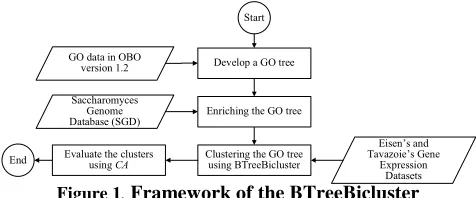
In the third chapter “Incorporating Gene Ontology with Conditional-based Clustering to Analyze

Gene Expression Data,” Shahreen Kasim, Safaai Deris, and Razib M. Othman proposed a

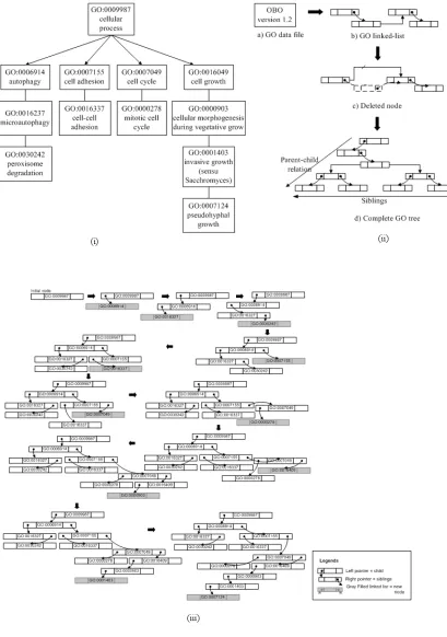
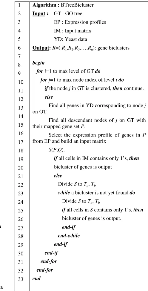
clustering algorithm named BTreeBicluster. The BTreeBicluster starts with the development of

GO tree and enriching it with expression similarity from the Sacchromyces genes. From the

enriched GO tree, the BTreeBicluster algorithm is applied during the clustering process. The

BTreeBicluster takes subset of conditions of gene expression dataset using discretized data.

Therefore, the annotation in the GO tree is already determined before the clustering process

starts which gives major reflect to the output clusters. Their results of this study have shown that

the BTreeBicluster produces better consistency of the annotation.

(4)

CHAPTER

TITLE

PAGE

ABSTRACT ………

ii

TABLE OF CONTENTS ……….………...

iv

1 Enhancement of Support Vector Machines for Remote Protein

Homology Detection and Fold Recognition

M. Hilmi Muda, Puteh Saad, and Razib M. Othman

……… 1

2 Hybrid Clustering Support Vector Machines by Incorporating

Protein Residue Information for Protein Local Structure Prediction

Rohayanti Hassan, Puteh Saad, and Razib M. Othman

……… 8

3 Incorporating Gene Ontology with Conditional-based Clustering

to Analyze Gene Expression Data

Shahreen Kasim, Safaai Deris, and Razib M. Othman

……….. 15

4 Improving Protein-Protein Interaction Prediction by a False Positive

Filtration

Process

(5)

Enhancement of Support Vector Machines for Remote

Protein Homology Detection and Fold Recognition

M. Hilmi Muda

Laboratory of Computational

Intelligence and Biology Faculty of Computer Science and

Information Systems Universiti Teknologi Malaysia, 81310

UTM Skudai, MALAYSIA +607-5599230

Puteh Saad

Department of Software Engineering Faculty of Computer Science and

Razib M. Othman

Intelligence and Biology Faculty of Computer Science and

ABSTRACT

Remote protein homology detection and fold recognition refers to detection of structural homology in proteins where there are small or no similarity in the sequence. The issues arise on how to accurately classify remote protein homology and fold recognition in the context of Structural Classification of Proteins (SCOP) hierarchy database and incorporate biological knowledge at the same time. Homology-based methods have been developed to detect protein structural classes from protein primary sequence information which can be divided into three types: discriminative classifiers, generative models for protein families and pairwise sequence comparisons. We present a comprehensive method based on two-layer multiclass classifiers. The first layer is used to detect up to superfamily and family in SCOP hierarchy, by using optimized binary SVM classification rules directly to ROC-Area. The second layer uses discriminative SVM algorithm with a state-of-the-art string kernel based on PSI-BLAST profiles that is used to leverage the unlabeled data. It will detect up to fold in SCOP hierarchy. We evaluated the results obtained using mean ROC and mean MRFP. Experimental results show that our approaches significantly improve the performance of protein remote protein homology detection for all three different datasets (SCOP 1.53, 1.67 and 1.73). We achieved 0.03% improvement in term of mean ROC in dataset SCOP 1.53, 1.17% in dataset SCOP 1.67 and 0.33% in dataset SCOP 1.73 when compared to the results produced by state-of-the-art methods.

Keywords

Fold recognition; Multiclass classifiers; Remote protein homology detection; Support vector machines; Two-layer classifiers.

1. INTRODUCTION

Advances in molecular biology in past years like large-scale sequencing and the human genome project, have yielded an unprecedented amount of new protein sequences. The resulting sequences describe a protein in terms of the amino acids that constitute it and no structural or functional protein information is available at this stage. To a degree, this information can be inferred by finding a relationship (or homology) between new sequences and proteins for which structural properties are already known. Traditional laboratory methods of protein homology detection depend on lengthy and expensive procedures like x-ray crystallography and nuclear magnetic resonance (NMR). Since using these procedures is unpractical for the amount of data available, researchers are increasingly relying on computational

techniques to automate the process. Accurately detecting homologs at low levels of sequence similarity (remote protein homology detection) still remains a challenging ordeal to biologists. Remote protein homology detection refers to detection of structural homology in proteins where there are small or no similarity in the sequence. To detect protein structural classes from protein primary sequence information, homology-based methods have been developed, which can be divided into three types: discriminative classifiers [2,10,15,16,25], generative models for protein families [13,21] and pairwise sequence comparisons [1]. Discriminative classifiers show superior performance when compared to other methods [16,23].

Support Vector Machines (SVM) and Neural Networks (NN) are two popular discriminative methods. Recent studies showed that SVM has faster training speed, more accurate and efficient compared to NN [4]. This classifier is uniquely different from generative models and pairwise sequence comparisons because it removes the amino acid sequence from the prediction step. The protein sequences are transformed into feature vectors and then are used to train an SVM to identify protein families. Feature vectors give the benefit of mapping the sequences into a multivariate representation and additionally do not depend on a single pairwise score.

The performance of remote protein homology detection has been further improved through the use of methods that explicitly model the differences between the various protein families (classes) and build discriminative models. In particular, a number of different methods have been developed that build these discriminative models based on SVM and have shown, provided there are sufficient data for training, to produce results that are in general superior to those produced by pairwise sequence comparisons or methods based on generative models [2,10,15,16,25], [15,7].

(6)

Details are explained in the methods section. We evaluated our result using mean ROC and mean RFP. Experimental results show that our approaches significantly improve the performance of protein remote protein homology detection.

2. METHODS

In this section, we will briefly explain our proposed method named SVM-2L to build two layers multiclass classifiers. Based on idea of Lorena and Carvalho [19] we tuned SVM’s parameters in our first layer multiclass classifier to influence their performance. They are the value of the regularization constant, C

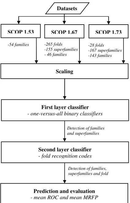
and kernel type, with its respective parameter. With the combination of the second layer multiclass classifier which uses the SVM with improved kernel based on PSI-BLAST profiles to leverage unlabeled data, it is expected to improve performance of remote protein homology detection and fold recognition by adding elements without overfitting. The overall steps of the SVM-2L is as shown in Figure 1.

2.1 Experimental Datasets

We evaluated the performance of our method using three datasets. The first dataset, SCOP version 1.53, we emulate the benchmark procedure presented by Liao and Noble [18]. The data consist of 4352 sequences extracted from the Astral [4] database grouped into families and superfamilies. For each family, the protein domains within the family are considered positive test examples, and protein domains within the superfamily but outside the family

are considered positive training examples. This yields 54 families with at least 10 positive training examples and five positive test examples. Negative examples for the family are chosen from outside of the positive sequences fold, and were randomly split into training and test sets in the same ratio as the positive example.

Second dataset are derived from SCOP version 1.67 created by Rangwala and Karypis [25]. Datasets fd25 were designed to evaluate the performance of fold recognition and were derived by taking only the domains with less than 25% pairwise sequence identity, respectively. This set of domains was further reduced by keeping only the domains belonging to folds that contained at least three superfamilies and at least three of these superfamilies contained more than three domains. For fd25, the resulting dataset contained 1294 domains organized in 265 folds, 155 superfamilies and 46 families.

We also tested our method on the latest version dataset from SCOP version 1.73. We follow the filtering step by Rangwala and Karypis [25] to select the dataset, which results 1597 domains organized in 28 folds and 167 superfamilies. We derived the dataset by taking only the domains with less than 95% and 40% pairwise sequence identity according to Astral database. This set of domain was further reduced by keeping only the domains belonging to fold that contained at least 3 superfamilies, and one of these superfamilies contained multiple families.

Dataset SCOP 1.53 contains superfamilies and families only, while datasets SCOP 1.67 and dataset SCOP 1.73 contains up to folds.

2.2 Scaling

Scaling the datasets before applying SVM is essential. The main advantage is to avoid attribute in greater numeric ranges dominate those in smaller numeric ranges. Other than that, it is also used to avoid numerical difficulties during the calculations. Because kernel values usually depends on the inner products of feature vectors, e.g. the linear kernel and the polynomial kernel in which large attribute values might result in numerical problems. We linearly scale each attribute to the range [-1, 1] [19]. Testing and training datasets must obviously be scaled using the same method. Suppose to scale a certain attribute of training dataset from

, min max

y y

[ ]to[y'_min, 'y_max], where y is the raw attribute value of training or testing datasets. The scaled value is obtained from Zheng et al. [34] as follows

'_max '_min ' '_min ( _min)

max min

y y y y y y

y y

−

= + −

− . (1)

2.3 First Layer Classifiers

The various one-versus-all binary classifiers were constructed using SVM. One of the implementations is SVMstruct[14] that train conventional linear classification SVM optimizing error rate in time that is linear in the size of the training data through an alternative, but equivalent formulation of the training problem. It implements the alternative structural formulation of the SVM optimization problem for conventional binary classification with error rate and ordinal regression. Moreover, SVMstruct used small memory (15500 Kilobytes) resource when training large set of data, which make it more efficient [21]. We used the formulation of the SVM optimization problem by Joachims [20] that provides the basis of our algorithm, both for classification and for ordinal regression SVM.

Datasets

SCOP 1.53 SCOP 1.67

First layer classifier

- one-versus-all binary classifiers

-265 folds -155 superfamilies - 46 families

-28 folds -167 superfamilies -143 families -54 families

Second layer classifier

- fold recognition codes

Prediction and evaluation

- mean ROC and mean MRFP

Detection of families and superfamilies

Detection of families, superfamilies and fold

SCOP 1.73

Scaling

(7)

2.3.1 Classification

For a given training dataset (x y_{1 1}, ),...,(x_n,y_n)with n length, x_i∈ℜN

where _ℜN_{a radical power of large of features,}_N_{is the large}

number of features, y is stated asy_i∈ − +{ 1, 1} training a binary classification SVM means solving the optimization problem [13]. For simplicity of the theoretical results (Eq. 2), we focus on classification rules h_w( ) sin(x= w x bT + )with b=0, where w is the empty stack of constraints, T is the iterations and b is regression loss. A non-zero b can easily be modeled by adding an additional feature of constant value to each x.

1 min

2

, 0 1

n C T w w _i

n w _i i

+ ∑ξ

ξ ≥ =

, (2)

where∀ ∈i{1,..., }:n y w x_i( T _i) 1≥ −ξ_i.

We adopted the formulation of [30], [33] where sum of linear slack variables, Σξ_i is divided by n length to better capture how trade-off between training error and margin, C, scales with the training set size. The Eq. 3 in the following considers a different optimization problem, which was proposed for training SVM to predict structured outputs as been done by Tsochantaridis et al. [30]. 1 min 2 , T w w C w

+ ξ

ξ≥0 , (3)

where {0,1} :1 1

1 1

n n n T

c w c y x_{i i i} c_i n _i n_i

∀ ∈ ∑ ≥ ∑ −ξ

= =

.

While Eq. 3 has 2n constraints, one of each possible vector c=(c ,...,c )₁ _n (x_{1 1},y ),...,(x_n,y_n), it only has one slack variable

ξ

that is shared across all the constraints. Each constraint in this equation corresponds to the sum of a subset of constraints from Eq. 1, and the

c

_i select the subset. 1

1

n c_i n i∑=

can be seen as the maximum fraction of training errors possible over each subset and ξ is an upper bound on the fraction of training errors made by _hw

.

2.3.2 Ordinal Regression

In an example(x y_i, _i), the label

i

y

indicates a rank instead of a nominal class in ordinal regression. We let y_i∈{1,..., }Z with Z

length, so that the values 1,...,Zare related on an ordinal scale, without loss of generality. The goal is to learn a function h x( ) so that for many pair of examples x_i,y_iandx_j,y_jit holds that

( ) ( )

h x_i >h x_j ⇔y_i>y_j. ₍₄₎ Given a training dataset (x y_{1 1}, ),...,(x_n,y_n) with x_i∈ℜNand

{( , ): }

P= i j y_i>y_j , formulate the ordinal regression SVM (Eq. 5). Denote with P the set of pairs ( , )i j for which example i has a

higher rank than example j, i.e.P={( , ):i j y_i>y_j}, and let m=| |P . 1

min 2

, 0 ( , )

C T

w w _ij m w _ij i j P

+ ∑ ξ

ξ ≥ ∈

, (5)

where ∀( , )i j∈P w x:( T _i) (≥ w xT _j) 1+ −ξ_ij.

These formulations find a large margin linear functionh x( ), which

minimizes the number of pairs of training examples that are swapped with respect to their desired order. As in other classification, Eq. 5 is a convex quadratic program. Ordinal regression problems have applications in learning retrieval functions for search engines [7, 27, 29]. Furthermore, if the labels

y takes only two values, Eq. 5 optimizes the ROC-Area of the classification rule.

2.4 Second Layer Classifiers

We used profile-based string kernel SVM that are trained to perform binary classifications on the fold and superfamily levels of SCOP as a base for our multi-class protein classifiers. The profile kernel defined as a function that is used to measure the similarity of two protein sequence profiles based on their representation in a high-dimensional vector space indexed by all

k-mers (k-length subsequences of amino acids).

Binary one-vs-the-rest SVM classifiers that are trained to recognize individual structural classes yield prediction scores that are incomparable, so that standard ”one-vs-all” classification performs sub optimally when the number of classes is very large, as in this case. We used fold recognition codes that learn relative weights between one-vs-the-rest classifiers and further, encode information about the protein structural hierarchy for multi-class prediction, as to deal with this challenging problem. In large scale benchmark results based on the SCOP database, our method significantly improves on the prediction accuracy of both a baseline use of PSI-BLAST and the standard one-vs-all method. The use of profile-based string kernels is an example of semi-supervised learning, since unlabeled data in the form of a large sequence database is used in the discrimination problem. Moreover, profile kernel values can be efficiently computed in time that scales linearly with input sequence length. Equipped with such a kernel mapping, one can use SVM to perform binary protein classification on the fold level and superfamily level.

2.4.1 Fold Recognition Code

Suppose that we have trained q fold detectors. Then, for a protein sequence x, we form a prediction discriminant vector

( ) (₁( ),..., ( ))

f x= f x f_q x

r

. The simple one-versus-all prediction rule for multi-class fold prediction isyˆ arg max= _jf_j( )x . The problem with this prediction rule is that the discriminant values produced by the different SVM classifiers are not necessarily comparable. We used an approach by learning the optimal weighting for a set of classifiers, scaling their discriminant values and making them more readily comparable. To fit the training datasets, we adapt the coding system by learning a weighting of the code elements (or classifiers). The final multi-class prediction rule is

ˆ arg max ( * ( )).

y= _jW f xr K_j, where * denotes the component-wise multiplication between vectors and W is a weight vector.

2.5 Evaluation Measures

(8)

Table 1: Mean ROC (a) and mean MRFP (b) for different methods for family and superfamilies using SCOP 1.53 dataset.

(a)

Method Family Superfamily Overall

SVM-2L 0.9998 0.9976 0.9345

SVM Struct 0.8987 0.9521 0.8543

SVM-Fold 0.9458 0.9424 0.9342

SVM-Pairwise 0.4380 0.4380

SVM-Fisher 0.4370 0.4370

SVM-HMMSTR 0.6400 0.6400

SVM-Ngram-LSA 0.8929 0.8992 0.9132

SVM-Motif-LSA 0.9995 0.9897 0.9335

SVM-Pattern-LSA 0.9964 0.9925 0.9264 (b)

Method Family Superfamily Overall

SVM-2L 0.0012 0.0019 0.0015

SVM Struct 0.0060 0.0002 0.0031

SVM-Fold 0.0018 0.0008 0.0013

SVM-Fisher 0.0963 0.0096 0.0486

SVM-Pairwise 0.1173 0.1173

SVM-HMMSTR 0.0380 0.0380

SVM-Ngram-LSA 0.1017 0.1017

SVM-Motif-LSA 0.9953 0.9953

SVM-Pattern-LSA 0.0703 0.0703

(a)

Method Family Superfamily Fold Overall

SVM-2L 0.9987 0.9991 0.9876 0.9951

SVM Struct 0.9458 0.9867 0.9753 0.9692

SVM-Fold 0.9532 0.9986 0.9986 0.9834

SVM-Ngram-LSA 0.9038 0.9645 0.9856 0.9513 SVM-Motif-LSA 0.8973 0.9979 0.9884 0.9612 SVM-Pattern-LSA 0.9234 0.9753 0.9981 0.9656

(b)

SVM-2L 0.00056 0.00087 0.00065 0.00208

SVM Struct 0.00063 0.00065 0.00074 0.00202

SVM-Fold 0.00087 0.00045 0.00053 0.00185

SVM-Ngram-LSA 0.00722 0.00056 0.00062 0.00840 SVM-Motif-LSA 0.00066 0.00076 0.00034 0.00176 SVM-Pattern-LSA 0.00099 0.00063 0.00024 0.00186 The ROC curve is obtained by plotting the True Positive Rate

(TPR) against the False Positive Rate (FPR), for the entire range of possible cutoff values, c. On this plot, the line through the origin with slope 1 would correspond to the performance of a similarity detection based on a random similarity score. A method which detects SCOP similarity better than randomly must show a ROC curve situated above this diagonal.

MRFP is a RFP median value of each protein sequences grouped in several families. Mean MRFP is MRFP average value for entire set of protein sequences families. The MRFP is bounded by 0 and 1 and is used to measure the error rate of the prediction under the score threshold where half of the true positives can be detected. These measures are used for evaluation cited in [12, 18].

3. Results and Discussion

As discussed in the introduction section, our research in this paper is motivated by the idea and work from Rangwala and Karypis

[26] and Ie et al. [10], by which they solve the classification problem in the context of remote homology detection and fold recognition. Based on their work, we presented a two-layer multiclass classifiers approach called SVM-2L. We compare our method with other eight different methods: SVM Struct [30], Fold [22], Pairwise [19], Fisher [11], SVM-HMMSTR [34], SVM-Ngram-LSA [6], SVM-Pattern-LSA [6] and SVM-Motif-LSA [31] that already has been used to detect remote protein homology. The performance of various schemes in term of mean ROC and mean RFP is shown in Table 1(a) and

Table 1(b) respectively for remote protein homology detection using standard benchmark dataset, SCOP 1.53. We split the results to the group of family and superfamily. The result of SVM-Pairwise, SVM-Fisher and SVM-HMMSTR are retrieved from [34]. We use publicly available SVM-Motif-LSA to search sequence databases for matches to motifs. Based on our results on mean ROC in Table 1, it shows that our proposed method significantly outperforms existing state-of-the-art methods. Comparison of results by group of family and group of superfamily also clearly shows that our proposed methods are really efficient. This scenario is influenced by the use of large margin SVM classifier and its discriminative approach that we

implemented in our framework. We find out that some of these results agree with previous assessments. For example, the relative performance of SVM-Fisher agrees with the results given by Jaakkola et al. [32]. Although in that work the difference was more pronounced and relative performance of SVM-Pairwise results given in [8].

(9)

(a)

(b)

Figure 2. Curve of Mean ROC (a) and mean MRFP (b) for dataset SCOP1.67.

(a)

(b)

Figure 3. Curve of Mean ROC (a) and mean MRFP (b) for dataset SCOP1.73.

(a)

SVM-2L 0.9118 0.8329 0.8295 0.9019

SVM Struct 0.8897 0.8495 0.8390 0.8871

SVM-Fold 0.8952 0.8952 0.9363 0.8295

SVM-Ngram-LSA 0.8746 0.8871 0.8615 0.8481 SVM-Motif-LSA 0.8592 0.8826 0.8273 0.8733 SVM-Pattern-LSA 0.8794 0.8979 0.8798 0.8986

(b)

SVM-2L 0.0386 0.0563 0.1443 0.0238

SVM Struct 0.0342 0.1724 0.1366 0.0304

SVM-Fold 0.1136 0.0967 0.0945 0.0303

SVM-Ngram-LSA 0.1390 0.1764 0.1157 0.0386 SVM-Motif-LSA 0.1411 0.1515 0.2075 0.0495 SVM-Pattern-LSA 0.1157 0.1600 0.4814 0.0437 For dataset SCOP 1.73, we achieve improvement of 0.14% which is depicted in Table 3(a) and Table 3(b). The mean ROC of our methods improves from state-of-the-art methods as depicted in Figure 3(a) and Figure 3(b). Although, there is only a slight improvement, however our proposed method demonstrates a

stable performance. This is the impact of using the fold detection codes which encodes information about the protein structural hierarchy for multi-class detection and the repetition of cross validation process in the first layer method. Meanwhile, in mean RFP result, our proposed method contributes 0.0072% better when compared to results produced by SVM Struct. When it is tested on dataset SCOP 1.73, it produces a lower error rate, as shown in good result in median rate of false positive in Table 3(b).

From stability of the curve of mean ROC and mean RFP in Figure 2 and Figure 3, we can conclude that our proposed method produced a stable result for all datasets. Even though for some point the curves show a low result, however it produces a positive effect to the result. Other than that, our method is consistent for all datasets. In summary, overall result from our method shows more than 0.9 in the term of mean ROC for all three different experimental datasets. We achieved 0.03% improvements in dataset SCOP 1.53, 1.17% in dataset SCOP 1.67 and 0.33% in dataset SCOP 1.73 when compared to the result produced by state-of-the-art methods.

4. Conclusion

(10)

with a state-of-the-art string kernel based on PSI-BLAST profiles to leverage unlabeled data. A number of different methods have been developed that build these discriminative models based on SVM and have shown, provided there are sufficient data for training, to produce results that are in general superior to those produced by pairwise sequence comparisons or methods based on generative models. The result produced by our method also shows good improvements in all three different datasets. In the future, we intend to enhance our method by using the realignment approach that will correct misalignments between a sequence and the rest of profile. Other than that, implementation of other kernel functions in SVM classifiers is hypothesized to improve the performance of remote protein homology detection and fold recognition, since different kernel function corresponds to different input.

5. ACKNOWLEDGMENTS

This project is funded by Malaysian Ministry of Higher Education (MOHE) under Fundamental Research Grant Scheme (project no 78092).

6. REFERENCES

[1] Altschul, S. F., Gish, W., Miller, W., Myers, E. W., and Lipman, D. J. 1990. ABasic Local Alignment Search Tool. Journal of Molecular Biology 215 (3), 403-410.

[2] Andreeva, A., Howorth., D., Chandonia, J., Brenner, S., Hubbard, T., Chothia C., and Murzin, A. (2008). Data growth and its impact on the SCOP database: new developments. Nucleic Acids Research. 36 (1), 419-425. [3] Ben-Hur, A and Brutlag D. 2003. Remote homology

detection: a motif based approach. In Proceedings of the International Conference on Intelligent Systems for Molecular Biology (Brisbane, Australia, June 29-July 3, 2003).

[4] Brenner, S., Koehl, P. and Levitt, M. 2000. The ASTRAL compendium for sequence and structure analysis. Nucleic Acids Research. 28 (1), 254-256.

[5] Ding, C.H.Q., and Dubchak, I. 2001. Multi-class protein fold recognition using support vector machines and neural networks. Bioinformatics. 17 (4), 349-358.

[6] Dong, Q., Wang, X., Lin, L. 2006. Application of latent semantic analysis to protein remote homology detection. Bioinformatics. 22 (3), 285-290.

[7] Haoliang, Q., Sheng, L., Jianfeng, G., Zhongyuan, H. and Xinsong, X. (2008) Ordinal regression for information retrieval. Journal of Electronics (China).25 (1), 120-124. [8] Hou, Y., Hsu, W., Lee, M.L. and Bystroff, C. 2003. Efficient

remote homology detection using local structure. Bioinformatics. 19 (17), 2294-2301.

[9] Hsu, C.W., Chang, C.C. and Lin, C.J. A practical guide to support vector classification, 2008.

<http://csie.ntu.edu.tw/~cjlin/papers/guide/guide.pdf >. [10]Ie, E., Weston, J., Noble, W.S. and Leslie, C. 2005.

Multi-class protein fold recognition using adaptive codes, In Proceedings of the International Conference on Machine Learning (Bonn, Germany, August 7-11, 2005). ACM Press, New York, NY, 329-336. DOI =

http://doi.acm.org/10.1145/1102351.1102393

[11]Jaakkola, T., Diekhans, M. and Haussler, D. 1999. Using the Fisher kernel method to detect remote protein homologies, In Proceedings of the International Conference on Intelligent Systems for Molecular Biology (August 6–10, 1999, Heidelberg, Germany). AAAI Press, 149-158. [12]Jaakkola, T., M. Diekhans and D. Haussler. 2000. A

discriminative framework for detecting remote protein homologies. Journal of Computational Biology. 7 (1-2), 95-114.

[13]Joachims, T. 2005. A support vector method for multivariate performance measures,In Proceedings of the International Conference on Machine Learning, (Bonn, Germany, 7-11 August, 2005). ACM Press, New York, NY, 377-384. [14]Joachims, T. 2006. Training linear SVMs in linear time, In

Proceedings of the ACM Conference on Knowledge Discovery and Data Mining (Philadelphia, USA, 20-23 August, 2006). ACM Press, New York, NY, 217-226. DOI= http://doi.acm.org/10.1145/1150402.1150429

[15]Krogh, A., Brown, M., Mian, I.S., Sjölander, K. and Haussler, D. 1994. Hidden Markov Models in Computational Biology: Applications to Protein Modeling. Journal of Molecular Biology. 235 (5), 1501-1531.

[16]Kuang, R., Ie, E., Wang, K., Siddiqi, M., Freund, Y. and Leslie, C. 2005. Profile kernels for detecting remote protein homologs and discriminative motifs, Journal of

Bioinformatics and Computational Biology. 13, 21-23. [17]Leslie, C., Eskin, E., Cohen, A., Weston, J., and Noble, W.S.

2004. Mismatch String Kernels for Discriminative Protein Classification.Bioinformatics. 20 (4), 467-476.

[18]Liao, L. and Noble, W.S. 2002. Combining pairwise sequence similarity and support vector machines for remote protein homology detection. In Proceedings of the Annual International Conference on Research in Computational Molecular Biology (Washington, USA, 18-21 April, 2002). ACM Press, New York, NY, 225-232. DOI=

http://doi.acm.org/10.1145/1150402.1150429

[19]Liao, L. and Noble, W.S. 2003. Combining pairwise sequence similarity and support vector machines for detecting remote protein evolutionary and structural relationships. Journal of Computational Biology 10 (6), 857-868.

[20]Lorena, A. C. and Carvalho, A.C.P.L.F.d. 2008. Evolutionary tuning of SVM parameter values in multiclass problems. Neurocomputing. 71 (16-18), 3326-3334.

[21]Mangasarian, O. and Musicant, D. 2001. Lagrangian support vector machines. Journal of Machine Learning Research. 1 (1), 161-177.

[22]Melvin, I., Ie, E., Kuang, R., Weston, J., Stafford, N. and Leslie, C. 2007. SVM-Fold: a tool for discriminative multi-class protein fold and superfamily recognition. BMC Bioinformatics. (8:S2).

[23]Murzin, A. G., Brenner, S.E., Hubbard, T., and Chothia, C. 1995. SCOP: a structural classification of proteins database for the investigation of sequences and structures. Journal of Molecular Biology. 247 (4), 536-540.

(11)

using multiple sequences detect twice as many remote homologues as pairwise methods. Journal of Molecular Biology. 284 (4), 1201-1210.

[25]Rangwala, H. and Karypis, G. 2005. Profile based direct kernels for remote homology detection and fold recognition. Bioinformatics. 21 (23), 4239-4247.

[26]Rangwala, H. and Karypis, G. 2006. Building multiclass classifiers for remote homology detection and fold recognition. BMC Bioinformatics. (7) 455.

[27]Runarsson, T.P. 2006. Ordinal Regression in Evolutionary Computation. Springer Berlin.

[28]Saigo, H., Vert, J. P., Ueda, N. and Akutsu, T. 2004. Protein homology detection using string alignment kernels. Bioinformatics. 20 (11), 1682-1689.

[29]Sch¨olkopf, B., Smola, A.J., Williamson, R.C. and Bartlett, P.L. 2000. New support vector algorithms. Neural Computation. 12 (5), 1207-1245.

[30]Schoelkopf, B. and Smola, A.J. 2002. Learning with kernels.

MIT Press.

[31]Timothy, L. B., Nadya, W, Chris, M. and Wilfred, W.L. 2006. MEME: discovering and analyzing DNA and protein sequence motifs. Nucleic Acids Research. (34), 369-373. [32]Tsochantaridis, I., Hofmann, T., Joachims, T. and Altun, Y.

2004.Support Vector Learning for Interdependent and Structured Output Space. In Proceedings of the International Conference on Machine Learning (Banff, Alberta, Canada, 4-8 July, 2004). ICML’04. ACM Press, New York, NY, 4- 823-830. DOI= http://doi.acm.org/10.1145/1015330.1015341 [33]Tsochantaridis, I., Hofmann, T., Joachims, T. and Altun, Y.

2005. Large margin methods for structured and interdependent output variables. Journal of Machine Learning Research. (6), 1453–1484

.

[34]Yuna, H., Wynne, H, Lee, M. L. and Bystroff, C. 2004. Remote homolog detection using local sequence-structure correlations. PROTEINS: Structure, Function, and Bioinformatics. 57 (3), 518-530.

(12)

HYBRID CLUSTERING SUPPORT VECTOR MACHINES BY

INCORPORATING PROTEIN RESIDUE INFORMATION FOR

PROTEIN LOCAL STRUCTURE PREDICTION

Rohayanti Hassan

Laboratory of Computational Intelligence and Biology Universiti Teknologi Malaysia, 81310

[email protected]

Puteh Saad

Department of Software Engineering Faculty of Computer Science and Universiti Teknologi Malaysia, 81310

[email protected]

Razib M. Othman

Intelligence and Biology Universiti Teknologi Malaysia, 81310

[email protected]

ABSTRACT

Protein local structure prediction can be described as prediction of protein secondary structure from protein subsequence. This protein subsequence or also known as protein local structure covers fragments of the protein sequence. In fact, it is easier to identify the sequence-to-secondary structure relationship using protein subsequence rather than use the whole protein sequence. Further, this relationship can be used to infer new protein fold, protein function and detect protein remote homolog. Due to its significance, a predictive algorithm named R-HCSVM is developed to predict protein local structure that works with following steps. Firstly, pre-process the input information for R-HCSVM. There are two types of input information needed namely protein residue score and protein secondary structure class. ResiduePatchScore information has been introduced as new method to pre-process protein residue score by combining protein conservation score that conserved rich functional information and protein propensity score that conserved rich secondary structural information. Hence, the protein residue score possess strength information that able to avoid bias scoring. Secondly, segment protein sequences into nine continuous length of protein subsequence. Next step which is highlighted another novel part in this study whereas a hybrid clustering SVM is introduced to reduce the training complexity. SOM and K-Means are integrated as a clustering algorithm to produce a granular input, while SVM is then used as a classifier. Based on the protein sequence datasets obtained from PISCES database, it is found that the R-HCSVM performs outstanding result in predicting protein local structure from a given protein subsequence compared to other methods.

Keywords

Protein local structure prediction, protein secondary structure, protein residue score, SOM K-Means, Support Vector Machines.

1. INTRODUCTION

Prediction of protein secondary structure using protein local structure has shown promising improvements [3], [41], [42]. Protein local structure primarily made up from segments of amino acid. In another words, protein local structures are also called as protein subsequence, protein fragments by Chen et al. [4], protein segments by Zhong et al. [41] and Zhong et al. [42] or protein local structural motifs by Karchin et al. [15] and Karchin et al. [16]. This protein local structure coded all information of native structure of a protein such as hydrophobicity, hydrophilicity,

electrostatic and hydrogen bonds interaction. Furthermore, information or called knowledge of this protein local structure can be used to infer how the protein interacts with other molecules, predict its structure as well as function. In fact, this knowledge facilitates to drug design.For example, Hu and Hu [12] aimed at designing small-molecule compounds that restore the normal function of p53-MDM2 (two protein targets in cancer research) and consequently reduce or eliminated certain forms of specific cancer.

Indeed, supervised machine learning based method for protein local structure prediction have shown strong generalization capability in handling nonlinear classification such as works done using Support Vector Machine (SVM) [18], Neural Network (NN) [21] and Hidden Markov Model (HMM) [23]. Nevertheless, it is not favorable for large-scale datasets due to the convex quadratic programming property which is NP-complete in the worst case. As a consequence, the training process will become decelerate. Several techniques have been proposed in order to solve this training complexity problem, for instance including chunking method [34], osuna decomposition method [26] and sequential minimal optimization method [29]. However, these techniques do not scale well of the training datasets. In related work, several techniques including random selection [2], bagging [37] and clustering analysis [35] are used as dataset selection to reduce the number of training datasets in order to accelerate the training process. Yet, the performance of training process is greatly depends on training datasets selection that may cause significance datasets are being overlooked. As a result, by decomposing a large-scale datasets into series of smaller datasets using clustering algorithm [19], [23], the training complexity can be reduced without overlook the significance dataset.

2. MOTIVATION

(13)

local structure accurately such as works done by Levitt and Chotia [20] who first proposed to classify thirty one globular proteins into four structural classes. In 1990’s, Liu and Chou [22] improved the definitions of structural classes by increasing the size of associated protein regions. In another related works, Wu and Kabat [39], Shenkin et al. [36] and Karlin and Brocchieri [17] have came up with varies method to quantify the residue conservation score in order to determine protein local structure accurately. However, these wet-lab methods needed a long time to execute all experiments and cost consuming.

Difficulties of determining protein local structures experimentally motivates researcher to come up with computational method. Machine learning algorithm is another dimension of computational method to predict protein local structure. On one hand, the superior of this method is depend on the information is being supplied and learned. Basically, there are two types of information are needed for this method to execute. One is known as feature vector and another one is known as feature class. Feature vector in a form of numerical value is represented by protein residue score. Meanwhile, feature class in a form of nominal value is represented by protein secondary structure class. A superior method is desired to pre-process these two features in order to ensure they are reliable and possess strong information. For instance, in order to quantify the protein residue score, it has

to avoid from bias scoring as a result of sequence redundancy without losing the important evolutionary and structural information. Protein residue score can be quantified using propensity score that based on the proportion of predominant secondary structure such as done in Levitt and Chotia [20], Chou and Fasman [6] and Constantini et al. [7]. Recently, most protein residue score is quantified through Multiple Sequence Alignment (MSA) process that based on its evolutionary information which is more conserved functional information. This type of protein residue score also known as protein conservation score and example works such as done by Sander and Scheneider [32], Mirny and Shakhnovich [24] and Goldenberg et al. [9].

Recently, progress has been made in protein local structure prediction method in order to address several issues. Sander et al. [33] proposed two types of discriminative models for protein local structure prediction which are hybrid K-Means with SVM and hybrid K-Means with Random Forest (RF) in order to reduce the training complexity. Nevertheless, the proposed hybrid K-Means with RF may decelerate the training process as a result of randomly sampling the training dataset. Furthermore, the proposed hybrid K-Means with SVM which also has been proposed by Zhong et al. [42], suffered from poor initialization method to form a quality cluster.

(14)

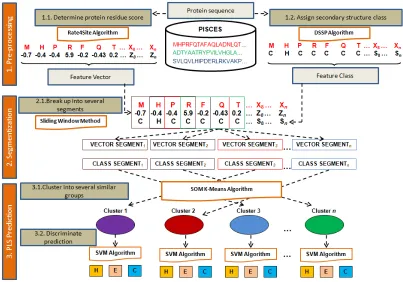
In fact, they adopted profile score from HSSP [32] database that only emphasized more on functional information to represent the protein residue score. On the other hand, Chen et al. [4] has proposed HYPLOSP to predict the local structure that based on Neural Network algorithm. Yet, they introduced high-scoring segment pairs for protein residue score that conserved more homology information rather than secondary structure information. Therefore, this study proposes a new algorithm to predict local structure named, R-HCSVM as shown in Figure 1. This R-HCSVM consists of two major components to (1) increase the strength of protein residue score and (2) reduce the training complexity. The R-HCSVM begins by determining the protein residue score using the first component named as ResiduePatchScore information. This ResiduePatchScore information ables to increase the strength information of protein residue score by combining protein conservation score that conserved rich functional information and protein propensity score that highly conserved secondary structure information. Subsequently, each of the protein sequence will be sliced into window segment to become feature vectors using sliding window method which has been implemented in Zhong et al. [42]. Next, DSSP method which was proposed by Kabsch and Sander [14] is used to assign secondary structure class to each protein residues. Besides, this study proposes granular SVM classification named as HCSVM in order to reduce the training complexity of predictive algorithm. Due to the large amount of protein subsequences being generated, Self-Organizing Map (SOM) is hybridized with K-Means to produce the granular input intelligently for SVM. This granular input allows SVM classification done in a series of tractable and simpler computationally problems. The detail explanation of the R-HCSVM can be found in the next section. Meanwhile, Receiver Operating Curve (ROC) and Segment Overlap (SOV) accuracy are used as metrics to evaluate the performance of the R-HCSVM in comparison to other similar algorithms. Experimental results show that R-HCSVM significantly improves the performance of protein local structure prediction.

The remainder of the paper consists of the detailed explanation of R-HCSVM (Section 2), description of the computational environment and data used in this study (Section 3), the results and discussion of experiments (Section 4), and the conclusions (Section 5).

3. METHODOLOGY

In this study, the proposed protein local structure prediction algorithm works as follows: (i) pre-process protein residue score information, (ii) pre-process protein secondary structure information, (iii) segmenting protein residue, (iv) classify protein subsequence for each granular input using SVM and (v) evaluate R-HCSVM using ROC and SOV.

3.1 Materials and Implementation

The dataset used in this study includes 2,000 protein sequences obtained from the PISCES [38] database. This dataset is the training dataset which is used to model the R-HCSVM. This protein database is bigger and more advanced than PDB-select-25 [11] that was used by Han and Baker [10]. Since PISCES uses PSI-BLAST [1] alignments to distinguish many underlying patterns below 40% identity, PISCES produces a more rigorous non-homologous database than PDB-select-25. In PISCES, the local alignment will not incorporate two proteins that share a common domain with sequence identity above the given

threshold. This feature helps to overcome problems of PDBREPRDB [25] database which uses global alignment that may generate useless sequence similarities. Meanwhile, to avoid the bias testing dataset, the k-fold cross validation is implemented. In this study, kf=10 is applied. Besides, one of the vectors used in this study is extracted from protein residue conservation score in Consurf server database which is available at http://consurfdb.tau.ac.il. Each of protein residue conservation score in alignment is calculated using Rate4Site algorithm. The advantages of this score as a result of implementation of phylogenetic relations between the aligned proteins and the stochastic nature of the evolutionary process explicitly. In addition, Rate4Site algorithm [30] assigns a conservation level for each position in MSA using an empirical Bayesian Inference. Whereby, the clustering process has been executed for six times to obtain the stable output clusters.

3.2 Pre-process Protein Residue Score

Information

As mentioned earlier, there are two types of protein residue score. One is determined by the propensity score based on the frequency occurrence of protein secondary structure. This score is outstanding in predicting protein secondary structure as a result of high structural conserved secondary structure information. To date, protein residue score is mostly determined based on its evolutionary history which is more functional conserved and known as protein conservation score. Besides, the advantage of this score is based on the superior Rate4Site algorithm that implements explicitly the phylogenetic relations between the aligned proteins and the stochastic nature of the evolutionary process through multiple sequence alignment in order to inherit highly conserved functional information and able to cater sequence redundancy. Therefore, this study is inspired to couple both protein residue score information named as ResiduePatchScore information in order to increase the strength of structural and functional conserved information. Further, the inaccurate prediction as consequence of bias protein residue score can be avoided. Four scores are employed to each protein residue. One is obtained from Consurf server database which is developed by Goldenberg et al. [9]. Meanwhile, the rest three scores are calculated based on its secondary structure propensity ratio in the whole dataset using Eq. 1. These secondary structure propensity scores clarify the degree of predominant role of H, E and C for each residue. Therefore, they were adopted in order to increase the strength of specified secondary structure information for each residue.

( / )

ab a

ab

b T

n n

P

N N

= , (1)

here, nabis the number of residues of type a in structure of type b, na is the total number of residues of type a, Nbis the total number of residues in structure of type b and NT is the total number of

residues in the whole dataset.

3.3 Pre-process Protein Secondary Structure

Class

(15)

(α-helix), G (310-helix), I (π-helix), E (β-strand), B (isolated

β-bridge), T (turn), S (bend) and the rest. However, in this study DSSP assigns each of residues using three larger classes of secondary structure namely H for helices, E for sheets and C for coils. The encoding secondary structure class is based on the following assignment: (i) H, G and I to H, (ii) E to E and (iii) the rest states to C.

3.4 Segmenting Protein Residue

Sliding window method is used to generate protein subsequence from 2,000 protein sequences. Each of protein subsequence composes of nine continuous residues. Therefore, it will generate up to 50,000 protein subsequences. In addition, many local structure prediction method use protein subsequence rather than the whole sequence itself during the prediction process. According to Chen et al. [5], the formation of helical structure can be affected by residues that are up to 9 positions away in the sequence, while the formation of coils and strands can be affected by residues that are up to 3 and 6 positions away respectively. The shorter formation structure in protein subsequence can yield noticeably improved the clustering process. Thus, this study generates the protein local segments with length of 9 residues to be known as protein local structure.

3.5 Clustering and Discriminate Protein

Local Structure

It is simpler and tractable to utilize SVM in multiple granular input spaces. Therefore, HCSVM contains two parts and works by: (1) group protein subsequences into several clusters using SOM K-Means and (2) classify protein subsequences in each clusters using SVM to identify the secondary structure class. The SOM is implemented first as a rough phase to reveal the similarity amongst protein subsequences. A vector quantization method in SOM able to simplify and reduces the training complexity in a SOM component plane as well as to discover the intrinsic relationship amongst protein subsequences. Next, K-Means is implemented as a refining phase on the learnt SOM to reduce the problem size of SOM cluster to the optimal number of K. The SVM classifier is subsequently used to train the protein subsequences in each cluster. Assume that a training protein subsequence S is given as;

{ , },_i _i 1...

S= x y i= n, (2)

where each xi is a feature vector and yi∈ − +{ 1, 1}corresponds to i

x label or feature class. The goal of SVM is to find the optimal hyperplane,

. ( )_i 0

wφ x + =b , (3)

in a high-dimensional space that able to separate the data from classes 1− and 1+ with maximal margin.

w

is a weight vector orthogonal to the hyperplane, b is a scalar and φ is a function which maps the data into a high-dimensional space also named as feature space. One merit of SVM is to map the input vectors into a high dimensional feature space and thus can solve the nonlinear case. The capability of SVM in handling the nonlinear relationship amongst protein subsequence is based on the nonlinear kernel function. The RBF is used as the nonlinear kernel function and defined as follows:

2

|| ||

( , ) exp( )

2

i j

r x x

K x x

σ

− −

= , (4)

where xi and xj are input vectors. The input vector will be the

centre of the RBF and σ will determine the area of influence this input vector has over the data space. A larger value of σ will give a smoother decision surface and more regular decision boundary since the RBF with large σ will allow an input vector to have a strong influence over a larger area.

3.6 Evaluate Prediction

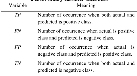
There are three secondary structure classes H, E or C will be determined or predicted for given protein subsequence. Meanwhile, the predictive algorithm in this study is based on binary classification which is presented in two classes for each secondary structure class. For example, to predict the protein subsequence as H class, positive class, +1 will be assigned to protein subsequence which is detected as H. Conversely, negative class, –1 will be assigned to protein subsequence which is detected as non H. Four possible outcomes will be generated from this classifier. The classification of these outcomes is described in contingency table 2x2 in Table 1.

Table 1. Contingency table 2x2 for binary classifier outcomes.

Actual H Actual non H

Predicted H True positives (TP) False negatives (FN)

Predicted non H

False positives (FP) True negatives (TN)

Further, Table 2 explains the definition of variables that used in Table 1. Later, these variables derived to the used in ROCl formula.

Table 2. The definition of variable used in contingency table 2x2 for binary classifier outcomes.

Variable Meaning

TP Number of occurrence when both actual and predicted is positive class.

FN Number of occurrence when actual is positive class and predicted is negative class.

FP Number of occurrence when actual is negative class and predicted is positive class.

TN Number of occurrence when both actual and predicted is negative class.

Basically ROC curve is used to visualize the performance of binary classifier in cartesian graph. Area under curve as shown in the following formula is another statistical index to describe the ROC measurement.

ROC = 1( )( )

2 TPR FPR , (7)

(16)

SOVH = 1 1

1 1

min{ ( , )} ( , )

1

max{ ( , )}

H

i N

i i i

i

H i i

OV s s s s

N OV s s

δ + +

= +

+

∑

, (8)

here, si and si+1 are the observed and predicted secondary structure

of local segments in the H state. NH is the total number of protein

local segments in H conformation. min{OV(si, si+1)} refers to the

minimum length of the actual overlap of si and si+1 and

max{OV(si, si+1)}is the maximum length of the total extent for

which either of the segments si or si+1 has a residue in H state.

Furthermore, the definition of δ(si, si+1) is as follows quoted by

Zemla et al. [40]:

1 1

1

max{ ( , )} min{ ( , )}

min{ ( , )}

( , ) min

int(0.5( ( ))) int(0.5( ( )))

i i i i

i

OV s s OV s s

OV s s s s len s len s δ + + + + + −       =        

, (9)

where, len(si) is the number of amino acid residues in segment. The similar calculation of SOV score in Eq. 8 will be applied to E and C state too.

4. RESULTS AND DISCUSSIONS

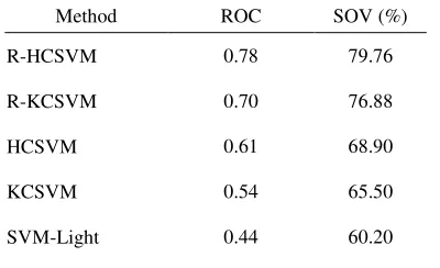
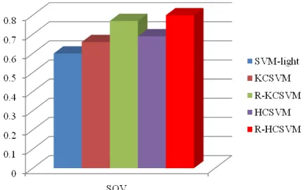
In this study, we test R-HCSVM and compare its performance with other methods such as SVM-light which is done by Joachims [13] that involves classifier alone, KCSVM which is introduced by Zhong et al. [42] that hybrid K-Means clustering algorithm and SVM classifier, R-KCSVM is a KCSVM with incorporates enriched protein residue score and HCSVM is a hybrid SOM K-Means clustering algorithm and SVM classifier without incorporates enriched protein residue score. Firstly, feature vector and feature class of R-HCSVM prediction method are pre-processed. Feature vector is represented using protein residue score which has been enriched by coupling the residue conservation score and residue propensity score based on secondary structure conserved information. On the other hand, feature class is represented by three states of secondary structure class which are generated using DSSP algorithm. Subsequently, all these feature vectors and classes are sliced in a window segment in prior to be discriminate using hybrid clustering SVM. Finally, the results generated by hybrid clustering SVM are evaluated. This evaluation provides a clear understanding of strengths and weaknesses of an algorithm that has been designed. The datasets of protein sequences obtained from PISCES database that have been defined in the previous section are used to test and evaluate the R-HCSVM and other protein local structure prediction methods. As depicted in Table 3 and emphasizes in Figures 2─3, using classifier alone which is represented by SVM-light produces the lowest accuracy per segment of 60.2% and average ROC of 44%. This is due to the high complexity of dataset inherits influence noise. In contrary, prediction method which implemented clustering algorithm at first hand shows better performance accuracy. Hybrid clustering SVM shows tremendous improvement of prediction method by revealing the sequence-to-local structure relationship in a smaller and tractable dataset. This is proved by KCSVM that increase 10% higher in ROC and 5.3% higher in accuracy per segment compared to prediction using SVM alone. Furthermore, sequence-to-local structure relationship is revealed in two levels learning process in HCSVM, where the first level is using SOM K-Means clustering algorithm and the second level is continued using SVM classifier. As a result, the sequence-to-local structure relationship process is more focused and the ROC as well as SOV is much higher with 17% and 8.6%

respectively compared to prediction using SVM alone. In addition, by enriching the information of protein residue score did improve the prediction method. This is due to the enriched protein residue score employed both high functionally and structurally conserved information which led to the increment of fraction score between the observed and predicted protein local segments. In R-KCSVM, the average ROC and SOV increased up to 16% and 11.38% respectively compared to prediction using KCSVM. Meanwhile, in R-HCSVM, the average ROC and SOV increased up to 17% and 10.86% respectively compared to prediction using HCSVM.

5. CONCLUSIONS AND FURTHER

WORKS

This paper discussed a computational method which is developed one is to increase the strength of protein residue score information and another one is to solve the training complexity of prediction algorithm in order to boost up the performance accuracy of protein local structure prediction. In the proposed computational method, there are two major machine learning algorithms are employed. One is SOM K-Means which is used to break up the complex dataset of protein local structures into several granular inputs or subspaces. Further, SVM classifier is implemented to each of generated granular inputs to learn and predict the protein local structure. In order to increase the strength of input information to this prediction algorithm, the protein residue score has been introduced which integrates protein conservation score and protein propensity score based on secondary structure information. The results from the evaluation phase in previous section shown that hybrid clustering SVM did improve the performance accuracy significantly compared to prediction algorithm that using classifier alone. Meanwhile, hybrid clustering SVM with incorporated enriched protein residue score is much improved the performance accuracy rather than using hybrid clustering SVM only.

Table 3. Performance comparison between R-HCSVM with other protein local structure prediction methods.

Method ROC SOV (%)

R-HCSVM 0.78 79.76

R-KCSVM 0.70 76.88

HCSVM 0.61 68.90

KCSVM 0.54 65.50

(17)

Figure 2. Performance comparison between R-HCSVM with other protein local structure prediction methods on ROC.

Figure 3. Performance comparison between R-HCSVM with other protein local structure prediction methods on SOV.

However, the performance accuracy specifically for sheets has a room to be improved. This study found that helices are the hardest to be captured in protein subsequence. One attempt to solve the problem is to enrich the secondary structure class information in order to capture more sheets occurrence. Besides, as a consequence of using binary classifier to predict three states of secondary structure class, unbalanced predicted class is occurred. Therefore, in future work, learning based secondary structure assignment will be proposed in order to capture more variability of secondary structure class and tertiary coding scheme will be integrated in order to solve the unbalanced predicted class.

6. ACKNOWLEDGMENTS

This work is funded by the Malaysian Ministry of Science, Technology and Innovation (MOSTI) under grant no. 01-01-06-SF0436. The authors sincerely thank reviewers for their comments on an earlier version of this manuscript.

7. REFERENCES

[1] Altschul, S. F., Madden, T. L., Schaffer, A. A., Zhang, J., Zhang, Z., Miller, W. and Lipman, D. J. (1997). Gapped BLAST and PSI–BLAST: A New Generation of Protein Database Search Programs. Nucleic Acids Research. 25(17): 3389–3402.

[2] Balcazar, J. L., Dai, Y. and Watanabe, O. (2001). Provably Fast Training Algorithms for Support Vector Machines. Proceedings of the IEEE International Conference on Data mining. November 29 – December 2, 2001. California, USA: IEEE Computer Society Press. 43–50.

[3] Bystroff, C., Thorsson, V. and Baker, D. (2000). HMMSTR: A Hidden Markov Model for Local Sequence–Structure Correlations in Proteins. Journal of Molecular Biology. 301(1): 173–190.

[4] Chen, C. T., Lin, H. N., Sung, T. Y. and Hsu W. L. (2006). Hyplosp: A Knowledge–Based Approach to Protein Local Structure Prediction. Journal of Bioinformatics and Computational Biology. 4(6): 1287–1308.

[5] Chen, K., Kurgan, L. and Ruan, J. (2006). Optimization of the Sliding Window Size for Protein Structure Prediction.

Proceedings of the IEEE Symposium on Computational Intelligence and Bioinformatics and Computational Biology. September 28-29, 2006. Ontario, Canada: Blackwell Publishing. 1–7.

[6] Chou, P. Y. and Fasman, G. D. (1978). Prediction of the Secondary Structure of Proteins from their Amino Acid Sequence. Journal of Advances in Enzymology and Related Areas of Molecular Biology. 47(1): 145–148.

[7] Constantini, S., Colonna, G. and Facchiano, A. M. (2007). PreSSAPro: A Software for the Prediction of Secondary Structure by Amino Acid Properties. Computational Biology and Chemistry. 31(5-6): 389–392.

[8] Frishman, D. and Argos, P. (1995). Knowledge–Based Protein Secondary Structure Assignment. Proteins. 23(4): 566–579.

[9] Goldenberg, O., Erez, E., Nimrod, G. and Ben-Tal, N. (2009). The ConSurf-DB: Pre-Calculated Evolutionary Conservation Profiles of Protein Structures. Nucleic Acids Research. 37(Database Issue): D323-D327.

[10]Han, K. F. and Baker, D. (1996). Global Properties of the Mapping Between Local Amino Acid Sequence and Local Structure in Proteins. PNAS. 93(12): 5814–5818.

[11]Hobohm, U. and Sander, C. (1994). Enlarged Representative Set of Protein Structures. Protein Science. 3(3): 522–524. [12]Hu, C. Q. and Hu, Y. Z. (2008). Small Molecule Inhibitors of

the p53–MDM2. Current Medical Chemistry. 15(17): 1720– 1730.

[13]Joachims, T. (1999). Making Large-Scale SVM Learning Practical. In: Scholkopf, B. and Burges, C. and Smola, A., Eds. Advances in Kernel Methods: Support Vector Learning. Cambridge, USA: MIT Press. 169–184.

[14]Kabsch, W. and Sander, C. (1983). Dictionary of Protein Secondary Structure: Pattern Recognition of Hydrogen– Bonded and Geometrical Features. Biopolymers. 22(12): 2577–2637.

[15]Karchin, R., Cline, M. and Karplus, K. (2004). Evaluation of Local Structure Alphabets Based on Residue Burial.

Proteins. 55(3): 508–518.