Conic Reformulations and Approximations to Some Subclasses of Nonconvex Quadratic Programming Problems.

ABSTRACT

DENG, ZHIBIN. Conic Reformulations and Approximations to Some Subclasses of Nonconvex Quadratic Programming Problems. (Under the direction of Dr. Shu-Cherng Fang.)

Conic Reformulations and Approximations to Some Subclasses of Nonconvex Quadratic Programming Problems

by Zhibin Deng

A dissertation submitted to the Graduate Faculty of North Carolina State University

in partial fulfillment of the requirements for the Degree of

Doctor of Philosophy

Industrial Engineering

Raleigh, North Carolina 2013

APPROVED BY:

Dr. Russell E. King Dr. James R. Wilson

Dr. Yunan Liu Dr. Shu-Cherng Fang

DEDICATION

This dissertation is dedicated to my family for their endless love and support: Yadi Le, my beloved wife

Rainee and Rachel Deng, my sweet daughters Shuying Cai, my dear Mom

BIOGRAPHY

ACKNOWLEDGEMENTS

Over the past four and half years I have received support and encouragement from a great number of individuals. Part of this work has been supported by the Edward P. Fitts Fellowship. I would like to express my deepest and sincerest gratitude to Dr. Shu-Cherng Fang for guiding me through my Ph.D. study. He inspired me not only in how to do researches, but also in how to be a responsible father. He showed me what is the best career path and helped me to achieve the goals. Great thanks also go to Dr. Russell E. King, Dr. James R. Wilson and Dr. Yunan Liu for their valuable comments as my committee members. I am thankful to Dr. Donald E.K. Martin for being the Graduate School Representative in my defense. I am also obliged to Dr. John E. Lavery and Dr. Wenxun Xing for their kindly help in my study.

Thanks to the staff of the Industrial and Systems Engineering Department, especially Ms. Cecilia Chen, Mr. Bill Irwin, Ms. Elaine Erwin and Mr. Justin Lancaster for their support and help. I am also grateful to my fellow friends in the FANGROUP: Pingke Li, Qingwei Jin, Kun Huang, Lan Li, Lu Yu, Yuan Tian, Ye Tian, Chia-Chun Hsu, Ziteng Wang, Jian Luo, Chien-Chia Huang, Tiantian Nie and many others whose names are not listed here. Their friendship and encouragement are always in my mind.

TABLE OF CONTENTS

LIST OF TABLES . . . vii

LIST OF FIGURES . . . .viii

Chapter 1 Introduction . . . 1

1.1 Statement of Problem and Motivation . . . 1

1.1.1 Quadratic Programming Problem over the Standard Simplex . . . 2

1.1.2 Quadratic Programming Problem over Convex Quadratic Constraints . . 2

1.1.3 Bounded Quadratically Constrained Quadratic Programming Problem . . 3

1.2 Approaches and Results . . . 3

1.3 Outline of the Dissertation . . . 4

Chapter 2 Preliminary Knowledge . . . 5

2.1 Notations . . . 5

2.2 QCQP and Linear Conic Programming Problems . . . 6

2.2.1 Some Examples . . . 9

2.3 Matrix Decomposition . . . 11

2.4 Duality Theory of LCoP Problems . . . 13

2.5 Linear Matrix Inequality and Reformulation-Linearization Technique . . . 14

2.5.1 Linear Matrix Inequality . . . 14

2.5.2 Reformulation-Linearization Technique . . . 15

Chapter 3 Quadratic Programming Problems over the Standard Simplex . . . 18

3.1 Introduction . . . 18

3.2 The cone of nonnegative quadratic functions . . . 20

3.2.1 A special case ofF . . . 21

3.3 Conic Reformulation and Approximation Cones . . . 22

3.3.1 Conic reformulation . . . 22

3.3.2 LMI based approximation cones . . . 24

3.4 Conic Approximation to Problem (StQP) . . . 26

3.5 An Adaptive Scheme for Detecting Copositive Matrices . . . 28

3.5.1 Sensitive points and sensitive ellipsoids . . . 28

3.5.2 An adaptive scheme . . . 30

3.5.3 Improving the lower bounds by RLT . . . 34

3.6 Numerical Examples . . . 34

3.7 Summary . . . 37

Chapter 4 Quadratic Programming Problems over Convex Quadratic Con-straints . . . 38

4.1 Introduction . . . 38

4.2 Conic Reformulation and Approximation to Problem (ETRS) . . . 39

4.3.1 An adaptive scheme for (ETRS) . . . 46

4.3.2 Proof of convergence . . . 50

4.4 Numerical Examples . . . 51

4.5 Computational Results . . . 54

4.6 Summary . . . 55

Chapter 5 Bounded Quadratically Constrained Quadratic Programming Prob-lems . . . 57

5.1 Introduction . . . 57

5.2 Range Reduction Strategy . . . 60

5.3 Cuts Generation . . . 61

5.3.1 Generalized Linear and Quadratic Polar Cuts . . . 61

5.3.2 Disjunctive Cuts . . . 65

5.4 A Branch-and-Cut Algorithm . . . 67

5.4.1 Pre-processing phase . . . 68

5.4.2 Branching step . . . 68

5.4.3 Cutting step . . . 69

5.4.4 The proposed algorithm . . . 70

5.5 Numerical Examples . . . 71

5.6 Conclusion . . . 75

Chapter 6 Conclusions. . . 76

6.1 Summary of Dissertation . . . 76

6.2 Future Research . . . 77

LIST OF TABLES

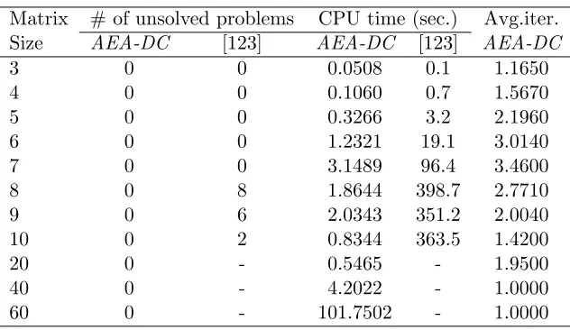
Table 3.1 Results of random test for AEA-DC . . . 36

Table 3.2 Simulation tests comparing with Yang et al. [123] . . . 36

Table 3.3 Results for simulation test of the form P+N. . . 37

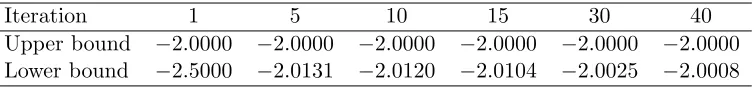
Table 4.1 The upper and lower bounds of Example 4.4.1. . . 52

Table 4.2 The upper and lower bound of Example 4.4.2. . . 53

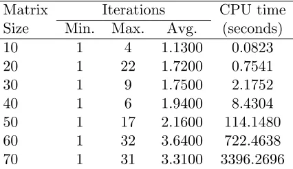
Table 4.3 Numerical results for 10 test problems. . . 55

Table 4.4 Numerical results for random generated instances . . . 55

Table 5.1 Comparison between BCA-BQCQPand Audet [13] . . . 72

Table 5.2 Comparison between BCA-BQCQPand Linderoth [72] . . . 73

Table 5.3 Characteristics of the test problems . . . 74

LIST OF FIGURES

Figure 2.1 Boundary of the positive semidefinite coneS2 +=

x y y z

. . . 10

Figure 2.2 Boundary of the copositive cone C2 = x y y z . . . 11

Figure 4.1 The upper and lower bounds of Example 4.4.1. . . 53

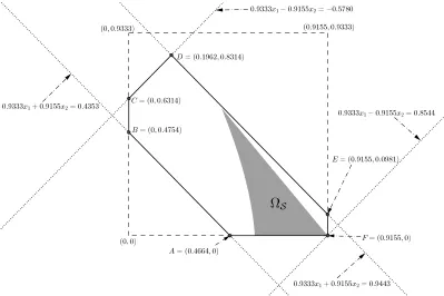
Figure 5.1 Graphic description for Example 5.3.1 . . . 66

Chapter 1

Introduction

Quadratically constrained quadratic programming (QCQP) forms an important class of opti-mization problems. The study of QCQP problems originated from Kuhn and Tucker [71] in 1951 and it is known that QCQP problems are NP-hard in general [85]. The aim of this dis-sertation is to study the theory of conic reformulations and approximations for solving some important subclasses of QCQP problems. Three fundamental subclasses of QCQP problems are particularly studied. The first one is the quadratic optimization over the standard simplex, the second one is the quadratic optimization over a set of convex quadratic constraints and the third one is the bounded quadratically constrained quadratic programming problem.

1.1

Statement of Problem and Motivation

A quadratically constrained quadratic programming problem can be defined as

(QCQP)

min xT_P0_{x+ 2(q}0₎T_x+γ0

s.t. xTPjx+ 2(qj)Tx+γj ≤0, j= 1, . . . , m,

(1.1)

where Pj _{∈ S}n_{, the space of real symmetric square matrices of order n, q}j _{∈ R}n_{, the}

1.1.1 Quadratic Programming Problem over the Standard Simplex A quadratic programming problem over the standard simplex has the following form:

(StQP)

min xTP0x

s.t. eTx= 1, x≥0,

(1.2)

wheree= (1, . . . ,1)T ∈_Rn_{. This problem is called the standard quadratic programming (StQP)}

in some literatures [22, 23, 24].

One notable application of problem (StQP) is the detection of copositivity of the matrix P0. Notice that the matrix P0 becomes copositive, if the optimal value of problem (StQP) is nonnegative. The concept of copositivity can be traced back to Motzkin [80] in 1952. Using the cone of copositive matrices in optimization for reformulating hard problems has been studied only in the last decade. A number of NP-hard problems, such as the binary quadratic problem [34], the fractional quadratic problem [92], determining the clique number of a graph [81], graph partitioning [90] and the quadratic assignment problem [91], have been shown to admit an exact copositive programming reformulation. Unfortunately, Murty and Kabadi [82] proved that detecting a copositive matrix is a co-NP-complete problem in 1987. Consequently, the development of approximation theory and efficient algorithms for detecting whether a given matrix is copositive or not are preliminary requirements for solving these hard problems.

1.1.2 Quadratic Programming Problem over Convex Quadratic Constraints A quadratic programming problem over a set of convex quadratic constraints has the following form:

(ETRS)

min xTP0x+ 2(q0)Tx

s.t. xTPjx+ 2(qj)Tx+γj ≤0, j = 1, . . . , m,

(1.3)

where P0 ∈ Sn _{and P}j _{∈ S}n

+, the space of real positive semidefinite matrices of order n, for j = 1, . . . , m. If m = 1, P1 is the identity matrix, q1 = 0 and γ1 < 0, then problem (ETRS) becomes the classical trust-region subproblem (TRS), which minimizes a nonconvex quadratic objective function over the unit ball. If m≥2, then the problem is called the extended trust-region subproblem (ETRS) [36].

problem (ETRS) could help develop efficient estimations for these combinatorial optimization problems. It also provides a better subroutine for solving nonlinear programming problems. However, there is no known polynomial-time algorithm for solving problem (ETRS) in general, even for the case that only one additional strictly convex quadratic constraint is added to TRS.

1.1.3 Bounded Quadratically Constrained Quadratic Programming Problem A bounded quadratically constrained quadratic programming (BQCQP) problem has the fol-lowing form:

(BQCQP)

min xTP0x+ 2(q0)Tx

s.t. xT_Pj_{x+ 2(q}j₎T_x+γj _{≤0, j = 1, . . . , m,}

l≤x≤u,

(1.4)

where Pj ∈ Sn_{; l, u and q}j _{∈ R}n _{for j = 0,1, ..., m; and γ}j _{∈ R for j = 1, . . . , m. Problem}

(BQCQP) is NP-hard in general because it generalizes many well-known NP-hard problems, such as mixed 0-1 linear programming [101] and bilinear programming [119].

Current methods for solving problem (BQCQP) are branch-and-bound (or branch-and-cut) algorithms with various relaxation schemes embedded [11, 13, 72]. The efficiency of these al-gorithms is mainly determined by the branch-and-bound (or branch-and-cut) rules and the tightness of the relaxation schemes. Therefore, development of a good estimation and an adap-tive branch-and-bound (or branch-and-cut) rule could lead to efficient algorithms for solving problem (BQCQP).

1.2

Approaches and Results

cone of nonnegative quadratic functions over the feasible domain of problem (ETRS) can also be introduced and similar approximation cones can be obtained based on a revised adaptive scheme. The approximation cones are further improved by using the reformulation-linearization technique (RLT). If the feasible domain of problem (ETRS) is bounded and has a nonempty interior, our proposed algorithm is shown to be able to find an -optimal solution in a finite number of iterations for any given small tolerance >0. The results for this part of work have been submitted [44].

Finally, we study the problem (BQCQP). The conic reformulation and serval convex re-laxations for the problem have been derived. A branch-and-cut algorithm based on linear and quadratic cuts is proposed to solve the problem. It is proven that the proposed algorithm yielded a globally r-z-optimal solution (with respect to feasibility and optimality, respectively) in a

finite number of iterations. In order to enhance the computational speed, an adaptive branch-and-cut rule is developed. The results for this work has been written in a working paper [46].

1.3

Outline of the Dissertation

Chapter 2

Preliminary Knowledge

Pardalos and Vavasis [85] proved that nonconvex quadratic programming problems are in gen-eral NP-hard. Therefore, problem (QCQP) defined in (1.1) is an NP-hard problem. In fact, some subcases of QCQP problems including the problem (StQP) defined in (1.2) and problem (ETRS) defined in (1.3) are NP-hard. Since we do not expect to have polynomial time algo-rithms in the literature for solving the QCQP problems, the existing algoalgo-rithms for solving problem (QCQP) can be generally divided into two categories:

1. Branch-and-bound algorithms based on the optimality conditions. The Karush-Kuhn-Tucker (KKT) conditions and other global optimality sufficient conditions are applied for designing branch rules while the lower bounds are derived from Lagrangian multipliers or convex relaxations. See [18, 33, 65, 120].

2. Branch-and-bound algorithms based on the convex relaxation and reformulation tech-niques. There exist various convex relaxation methods for nonconvex quadratic func-tions. Some good examples are linear programming relaxation, semidefinite programming (SDP) relaxation, second-order cone relaxation and reformulation-linearization techniques (RLT). See [13, 62, 72, 94, 102].

In the rest of this chapter, useful notations, related theory and techniques and major results are introduced for us to study the QCQP problems.

2.1

Notations

feasible domain is defined as the set of feasible solutions whose objective values are strictly greater than −∞. The optimal value of an optimization problem (P) is denoted by V(P).

Given an optimization problem (P), let its feasible domain beF_P ⊆_Rn_{. For anyx∈ F} P, if

there exists an open subset ofF_P containingx, then this open set is a neighborhood ofxand x is an interior point of FP. The set of all interior points is called the interior of FP, denoted by

int(F_P). The smallest closed set containingF_P is called the closure ofF_P, denoted bycl{FP}.

We have

int(FP)⊆ FP ⊆cl{FP}and cl{int(FP)}=cl{FP}.

The notation Sn _{denotes the set of real symmetric matrices of order n, S}n

+ denotes the set of positive semidefinite matrices of ordern, and Sn

++ denotes the set of positive definite matrices of ordern. For two real symmetric matrices A= (Aij) and B= (Bij) in Sn, the inner product

of Aand B is defined by

A•B =

n

X

i=1

n

X

j=1

AijBij. (2.1)

2.2

QCQP and Linear Conic Programming Problems

A coneK is a subset of a given space that satisfies

λx∈ K for all x∈ Kand λ≥0.

IfK has the property of

“x∈ K and −x∈ K” if and only if “x= 0”,

then it is apointedcone. The coneKissolidif it has a nonempty interior. IfKis pointed, solid, closed and convex, then we say the coneK isproper.

Given a set F ⊆_Rn_{, the convex hull ofF, denoted by}

conv{F }, is defined as the smallest convex set containingF, and theconic hullofF, denoted bycone{F }, is defined as the smallest convex cone containingF. From [28], we know

conv{F }=

x∈_Rn

x=

r

X

i=1

αixi for somer ∈N, xi ∈ F, 0≤αi≤1,

i= 1, . . . , r, such that

r

X

i=1 αi = 1

and

cone{F }= (

x∈_Rn

x=

r

X

i=1

αixi for somer ∈N, xi∈ F, αi ≥0 and i= 1, . . . , r

) ,

whereNis the set of positive integers. It is not difficult to see that

conv{F } ⊆cone{F } andcone{conv{F }}=cone{F }.

Given a coneK, a linear conic programming (LCoP) problem is defined as

(LCoP)

min C·X

s.t. Ai·X=bi, i= 1, . . . , m,

X ∈ K

(2.2)

where the notation “·” is the inner product in the relevant space. Among all the linear conic programming problems, three subclasses are widely used in theoretical study and practical com-puting. They are linear programming (LP) problems, second order cone programming (SOCP) problems and positive semidefinite programming (SDP) problems.

In an LP problem, K=Rn+,C,X,Ai,i= 1, . . . , m, are vectors in Rn,b= (b1, . . . , bm)T ∈

Rm and the inner product ·is defined byX·Y =XTY. In an SOCP problem, K ={[_xt]∈_Rn+1

t2 ≥xTxfort ∈ R+ andx ∈ Rn} ⊆Rn+1 is the second order cone, C, X,Ai, i= 1, . . . , m, are vectors in Rn+1, b = (b1, . . . , bm)T ∈Rm and

the inner product·is defined by X·Y =XTY. In an SDP problem,K=Sn

+,C,X,Ai,i= 1, . . . , m, are matrices inSn,b= (b1, . . . , bm)T ∈

Rm and the inner product ·is defined byX·Y =X•Y as defined in (2.1).

All these three types of problems can be solved in polynomial time (ref. [28, 48, 124]).

In order to derive the dual problem of (LCoP), we need the concept of dual cone. The dual set of a nonempty set F is defined as

F∗ =x x·y≥0 for ally ∈ F . (2.3)

Note thatF∗ _{is always a closed and convex cone. When F =K is a cone, the dual coneK}∗ _of

K is defined as

K∗ =x x·y≥0 for ally ∈ K . (2.4) Dual cones satisfy the following properties:

• K∗ _{is closed and convex.}

• IfK is solid, then K∗ _{is pointed.}

• If the closure of K is pointed, thenK∗ _{is solid.}

• (K∗₎∗ _{is the closure of the convex hull of K.}

These properties show that ifK is a proper cone, then so is its dualK∗ _{and (K}∗₎∗ _=K. By using the concept of dual cone, the dual problem of (LCoP) has the following form

(LCoD) max b

T_y

s.t. C−Pm

i=1yiAi ∈ K∗

(2.5)

Since the proper cones have more desirable properties, without any specific statement, we assume that K andK∗ _{are proper in problems (LCoP) and (LCoD), respectively, in the rest of} this chapter.

Sturm and Zhang [117] established the equivalence relation between quadratic programming problems and linear conic programming problems. In fact, any quadratic optimization problem has an equivalent linear conic programming problem form. In order to establish this equivalence relation, we need two concepts:homogenizationand thecone of nonnegative quadratic functions. Formally, for a nonempty set F ⊆_Rn_{, its homogenization is given by}

HF :=cl ("

t x #

∈_R++×_Rn

x/t∈ F

)

, (2.6)

which is a closed cone (not necessary to be convex though) in Rn+1. The cone of nonnegative quadratic functions over F is given by

NF := ("

z0 zT

z Z

#

∈ Sn+1

xTZx+ 2zTx+z0≥0 for allx∈ F )

, (2.7)

whereZ ∈ Sn_,z∈Rn _{and z0 ∈R. It was proved by Sturm and Zhang [117] that the coneN}

F can be represented by vectors fromHF. We state the result in the next theorem.

Theorem 2.2.1. For any nonempty set F, it holds that

NF = conv

yyT y∈H_F ∗

. (2.8)

By using the fact that

(see Lemma 3.1 in [73] or Lemma 1 in [117]) andHF is a closed cone, we can dualize Theorem 2.2.1 to get

N∗

F =conv{yyT|y∈HF}. (2.10)

Especially, whenF is closed and bounded, we have

N ∗

F =cone (

yyT

y= "

1 x #

, x∈ F

)

. (2.11)

For the following nonconvex quadratic programming problem (NQP):

(NQP) inf x

T_P0_{x+ 2(q}0₎T_x+γ0

s.t. x∈ F, (2.12)

where ∅ 6= F ⊆ _Rn _{is a possibly nonconvex domain, it is equivalent to the linear conic}

pro-gramming problem (MP) defined as

(MP) inf

"

γ0 _(q0₎T

q0 P0 #

•Z

s.t. Z11= 1, Z ∈N_F∗.

(2.13)

In principle, the nonconvex quadratic problem (NQP) and the convex problem (MP) are equiv-alent. But the fact that we can reformulate a general nonconvex problem (NQP) into a linear conic problem (MP) does not necessarily make such a problem easier to solve. In fact, all the implicit “difficult” constraints originating from the feasible domainF are packed into the cone N ∗

F. Only if we can efficiently solve problem (MP) and decompose the optimal solution of (MP) to get a solution of problem (NQP) in polynomial time, then we can say that there exists an efficient algorithm for solving the original problem (NQP).

2.2.1 Some Examples

In this subsection, two cones of nonnegative quadratic functions are studied. The first one is the well-known positive semidefinite cone.

Theorem 2.2.2. N_Rn=S₊n+1=N_R∗n.

Proof. It is easy to see that S₊n+1 ⊆ N_Rn. On the other hand, if there is a nonzero matrix U =

"

U11 uT u U¯

#

∈N_Rn\ S₊n+1whereU11∈R,u∈Rn, and ¯U ∈ S₊n, then there exists a nonzero

vectory= "

t x #

Ift6= 0, then yTU y=t2 " 1 x/t #T U " 1 x/t #

<0. This contradicts the assumption thatU ∈NF. Ift= 0, thenyTU y=xTU x <¯ 0. Considering the vectorλx∈_Rn_{withλ >0 being sufficiently}

large, we have

" 1 λx #T U " 1 λx #

=U11+ 2λuTx+λ2xTU x <¯ 0

where the last inequality holds because xTU x <¯ 0 and λis sufficiently large. This contradicts the assumptionU ∈N_Rn. Therefore,N_Rn =S₊n+1. Moreover, by using the fact that (S₊n+1)∗=

S₊n+1, we have N_R∗n = (S₊n+1)∗ =S₊n+1. See Figure 2.1 for the plot of S2

+. 0.0 0.5 1.0 1.5 2.0 x -1 0 1 y 0.0 0.5 1.0 1.5 2.0 z

Figure 2.1: Boundary of the positive semidefinite cone S2 +=

_{x y}

y z

.

The second one is thecone of copositive matrices

Cn=

M ∈ Sn

xTM x≥0 for allx∈Rn₊ . (2.14) Its dual cone, the completely positive cone, is defined as

C∗_n= (

M ∈ Sn M =

r

X

i=1

xi(xi)T for some r∈_N, xi ∈_Rn₊ and i= 1, . . . , r )

Notice that C∗

n S+n Cn.

Theorem 2.2.3. N_Rn

+ =Cn+1 and N

∗

Rn

+ =C

∗

n+1.

Proof. For any x ∈_Rn

+ and U ∈ Cn+1, " 1 x #T U " 1 x #

≥0 holds by the definition of C_n+1. Thus,

Cn+1 ⊆NRn

+. On the other hand, the same argument in Theorem 2.2.2 applies here except that

the vector y is in Rn++1 instead of in Rn+1. This proves that NRn

+ =Cn+1. By dualizing both

NRn

+ and Cn+1, we have N

∗

Rn

+ =C

∗

n+1.

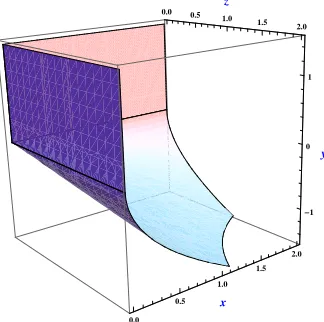
See Figure 2.2 for the plot of the boundary ofC₂.

0.0 0.5 1.0 1.5 2.0 x -1 0 1 y 0.0 _0.5 1.0 _1.5 2.0 z

Figure 2.2: Boundary of the copositive coneC2= x y

y z

.

2.3

Matrix Decomposition

Since an efficient algorithm for decomposing a matrix into desired vectors is important in obtain-ing the optimal solution of problem (NQP), we review some results about matrix decomposition in this section. Related results can be found in [4] and [125].

For any X∈ Sn

+,X has a rank-one decomposition, that is

X =

r

X

i=1

xi(xi)T

the decomposition exists without any doubt for each X ∈ Sn

+, this decomposition may not satisfy additional conditions, such as (xi)TY xi ≤ 0, i = 1, ..., r, for a given matrix Y ∈ Sn_.

The following theorem says that such decomposition does exist and it can be accomplished in polynomial time. This result is referred to [125].

Theorem 2.3.1. LetY be a given symmetric matrix inSn_{andX be a positive semidefinite}

ma-trix with rankr, 0< r≤n. Suppose thatX•Y ≤0, then there exists a rank-one decomposition of X running in polynomial time to find xi _∈Rn_{, i= 1, . . . , r, such that}

X=Pr

i=1xi(xi)T,

(xi)TY xi≤0, i= 1, ..., r. (2.16)

In particular, one can always find xi,i= 1, . . . , r, in polynomial time such that

X =Pr

i=1xi(xi)T,

(xi)TY xi =X•Y /r, i= 1..., r. (2.17)

The proof of Theorem 2.3.1 in [125] is a constructive one, which indicates that the decom-position can be achieved in polynomial time. The following theorem from [4] deals with a more complicated case in which two equality constraints need to be satisfied.

Theorem 2.3.2. Let Y1, Y2 be any two symmetric matrices in Sn _{and X = x}1_(x1₎T _{+· · ·+}

xr(xr)T with3≤r ≤n. If there exist δ1 and δ2 satisfying

(x1)TY1x1 = (x2)TY2x2 =δ1,

((x1)TY2x1−δ2)((x2)TY1x2−δ2)<0

(2.18)

then one can find a vector x˜1 ∈_Rn _{in polynomial time such that X = ˜x}1_(˜x1₎T _{+· · ·+ ˜x}r_(˜xr₎T

and

(˜x1)TY1x˜1 =δ1, (˜x1)TY2x˜1 =δ2.

(2.19)

2.4

Duality Theory of LCoP Problems

Problem (QCQP) is a special case of problem (NQP), hence it can also be reformulated as a linear conic programming problem, which has the same form as (MP) defined in (2.13). Consequently, the optimality conditions and duality properties of (LCoP) are useful in solving problem (QCQP). In this section, we review the optimality conditions and duality theorems of linear conic programming problems. For the optimality conditions and duality properties on nonlinear conic programming problems, one may refer to [6, 7, 40, 86, 112, 113, 114, 115].

First, we introduce the weak duality theorem for problem (LCoP).

Theorem 2.4.1 (Weak Conic Duality Theorem). Assume that problems (LCoP) and (LCoD)

are both feasible. Then, the optimal value of problem (LCoD) is a lower bound for the optimal value of problem (LCoP).

The weak duality theorem for problem (LCoP) is much weaker than the duality theorem for linear programming (LP). For LP problems, as long as both primal and dual problems are feasible, then we actually have the strong duality property, i.e., the optimal values of the primal and dual problems are equal. However, in order to get a similar strong duality result for problem (LCoP), we require the condition that the primal problem (LCoP) isstrictly feasible, i.e., there exists an X ∈int(K) such that Ai·X=bi fori= 1, . . . , m. Geometrically

speaking, A ∩int(K) 6= ∅, where A = {XA_i ·X = b_i, i = 1, . . . , m} is an affine space. Similarly, we say problem (LCoD) is strictly feasible if there existsy= (y1, . . . , ym)T such that

C−Pm

i=1yiAi∈int(K∗). Then we have the next strong duality theorem.

Theorem 2.4.2 (Strong Conic Duality Theorem). Consider problem (LCoP) defined in(2.2)

along with its conic dual problem(LCoD) defined in (2.5).

a. If problem (LCoP)is bounded below and strictly feasible, then problem(LCoD) is feasible, an optimal solution is attainable for problem (LCoD) and the optimal values of problems

(LCoP) and (LCoD) are equal.

b. If problem(LCoD)is bounded above and strictly feasible, then problem (LCoP)is feasible, an optimal solution is attainable for problem (LCoP) and the optimal values of problems

(LCoP) and (LCoD) are equal.

Based on the strong conic duality theorem, the conic optimality conditions for a primal-dual feasible pair (X∗, y∗) can be derived. The result is similar to the optimality conditions for LP problems.

Corollary 2.4.3 (Conic Optimality Conditions). Assume that at least one of the problems

is a pair of optimal solutions to the respective problems if and only if

C·X∗ =bTy∗ (zero duality gap)

or

X∗· C−

m

X

i=1 y∗_iAi

!

= 0 (complementary slackness)

For more results on the conic duality theories, one may refer to [20] and [28].

2.5

Linear Matrix Inequality and Reformulation-Linearization

Technique

In this section, we introduce two important tools that will be used in the rest of this dissertation.

2.5.1 Linear Matrix Inequality

A linear matrix inequality(LMI) is an expression of the form

A0+y1A1+· · ·+ymAm<0 (2.20)

where A0, . . . , Am are given n×n symmetric matrices, y = (y1, . . . , ym) is a vector of real

variables, and<is an order on Sn

+,i.e.,B <0 meansB is a positive semidefinite matrix. The history of LMIs can go back to 1890 when Lyapunov published his seminal work introducing what we now call Lyapunov theory. In 1940s, Lur’e et al. applied LMIs to important (and difficult) practical problems in control engineering [76]. But only small size LMIs can be solved “by hand.” In 1960s, Yakubovich et al. showed how to solve a certain family of LMIs by graphical methods [121, 122]. In late 1980s, Nesterov and Nemirovskii developed interior-point algorithms for solving LMIs [84]. Several interior-point algorithms have been implemented and tested on specific families of LMIs that arise in control theory, and found to be extremely efficient. For the more detailed history of LMIs, one may refer to [27].

There are two reasons to study LMIs in this dissertation:

(i) The form of an LMI is very general. Linear inequalities, convex quadratic inequalities, matrix norm inequalities and various other inequalities can all be rewritten as LMIs [119]. This is very useful when deriving the conic reformulations of QCQP problems. For example, an elliptic constraint described by

where Q ∈ Sn

++ and xc ∈ Rn can be expressed by the following LMI using the Schur

complement lemma [28]:

"

1 (x−xc)T

(x−xc) Q

#

<0.

(ii) An LMI is a convex constraint and can be solved efficiently [50]. Consequently, addi-tional LMI constraints in convex optimization problems (such as semidefinite program-ming problems) will not increase the complexity. This is very useful when developing conic approximations to QCQP problems. By adding some LMI constraints to an SDP problem used to estimate the original QCQP problem, we may obtain a better bound. Here, LMI constraints actually play a role of valid inequalities for solving SDP problems.

2.5.2 Reformulation-Linearization Technique

In this subsection, we describe a technique, calledreformulation-linearization technique(RLT), which generates LMIs for SDP problems. A recent review paper on RLT can be referred to [108].

RLT originated in [1, 2, 3]. It initially focused on solving 0-1 and mixed 0-1 linear and polynomial programming problems [100, 101] and later branched into the more general family of continuous, nonconvex polynomial programming problems [103, 104, 107]. The RLT essentially consists of two steps: a reformulation step in which certain additional nonlinear valid inequalities are automatically generated, and a linearization step in which each product term is replaced by a single continuous variable. Here is an example to demonstrate the procedure of RLT. Example 2.5.1. Consider the following box constrained nonconvex quadratic programming problem: (BQP) min    x1 x2 x3    T _  

−25 −1500 858

−1500 −1 −14

858 −14 −51       x1 x2 x3   +    3112 −4 162    T _   x1 x2 x3   

s.t. 0≤x1 ≤1, 0≤x2≤1, 0≤x3≤1.

The SDP relaxation for problem (BQP), due to Shor [110], has the following form: (BQP-SDP) min      

1 1556 −2 81

1556 −25 −1500 858

−2 −1500 −1 −14

81 858 −14 −51

      •      

1 x1 x2 x3

x1 X11 X12 X13 x2 X21 X22 X23 x3 X31 X32 X33      

s.t. 0≤x1 ≤1, 0≤x2≤1, 0≤x3 ≤1,      

1 x1 x2 x3 x1 X11 X12 X13 x2 X21 X22 X23 x3 X31 X32 X33       <0.

The optimal value of problem (BQP-SDP) is −179.0641, which is a lower bound for prob-lem (BQP). The reformulation step in RLT generates the following LMIs (or valid nonlinear inequalities):

xi(xj−1)≤0, i, j∈ {1,2,3}

from the constraints 0≤xi, xj ≤1 fori, j = 1,2,3. The linearization step in RLT replaces the

product termsxixj by a single variableXij fori, j= 1,2,3, leading to the linear inequalities:

Xij −xi ≤0, i, j ∈ {1,2,3}.

Therefore, after applying RLT, we arrive at a new relaxation problem:

(BQP-RLT) min      

1 1579 −109 −40 1579 −103 −1506 −17

−109 −1506 151 27

−40 −17 27 −48

      •      

1 x1 x2 x3 x1 X11 X12 X13 x2 X21 X22 X23 x3 X31 X32 X33      

s.t. 0≤x1 ≤1, 0≤x2≤1, 0≤x3 ≤1,      

1 x1 x2 x3

x1 X11 X12 X13 x2 X21 X22 X23 x3 X31 X32 X33       <0,

X11−x1 ≤0, X22−x2≤0, X33−x3 ≤0, X12−x1 ≤0, X12−x2≤0, X13−x3 ≤0, X13−x1 ≤0, X23−x2≤0, X23−x3 ≤0.

while problem (BQP-RLT) is polynomial-time solvable.

Chapter 3

Quadratic Programming Problems

over the Standard Simplex

In this chapter, we focus on quadratic optimization problems over the standard simplex and its application to the detection of copositive matrices. A sequence of linear conic programming problems are solved to approximate the original problem by using the semidefinite program-ming techniques. An adaptive approximation scheme is developed to speed up the convergence and relieve the computational effort of the proposed algorithm. Numerical examples and com-putational results are reported at the end of this chapter.

3.1

Introduction

A real n×n matrix M is copositive if the homogeneous quadratic form xTM x ≥ 0 for all x ∈ _Rn

+ = {x ∈ Rn|x ≥ 0}. Since the copositivity of a nonsymmetric matrix M can be determined by detecting a corresponding symmetric matrix M+₂MT, we assume that the given matrixM is symmetric in this chapter. The copositive coneCnis a cone consisting of alln×n

copositive matrices, and obviously Sn

+ ⊆ Cn. Recall that the inner product of two matrices A,

B ∈ Sn _{is defined as A•B = tr(A}T_{B) =}Pn

i=1 Pn

j=1AijBij. The dual cone of Cn, denoted by

C_n∗ ⊆ Sn_{, is the so-called completely positive cone.}

The study of copositivity can be traced back to Motzkin [80] in 1952. Both of the cones C_n

andC_n∗ are found to be useful in quadratic and combinatorial optimization. For example, Quist et al. [93] suggested that a stronger convex relaxation for a general quadratic programming problem can be derived by using the copositive cone C_n rather than the positive semidefinite cone Sn

therein. As to the applications to combinatorial optimization, de Klerk and Pasechnik [69] derived a copositive formulation for determining the stability number of a graph. Gvozdenovi´c and Laurent found a copositive formulation for the chromatic number of a graph in [56]. Other references include [47] and [90].

Checking whether a given matrix is copositive is proven to be co-NP-complete by Murty and Kabadi in [82]. For a matrix with a special structure, such as being tridiagonal and acyclic, checking its copositivity is possible in linear time ([21] and [64]). For symmetric matrices of order no more than 5, Andersson et al. [10] gave the necessary and sufficient conditions to determine copositivity. Hiriart-Urruty and Seeger [59] wrote a review on copositivity criteria based on matrix structural properties. The above approaches are only suitable for detecting the copositivity of moderate size matrices because of computational requirements. For this purpose, Bundfuss and D¨ur [31] proposed using global optimization techniques to check copositivity. Their criterion arises from the representation of the quadratic form in barycentric coordinates with respect to the standard simplex and its simplicial partitions thereof. As the partition gets finer and finer, all strictly copositive matrices are captured. This approach gives very good numerical results for many matrices. Most recently, Bomze and Eichfelder [25] present three new copositivity tests based on the difference-of-convex (d.c.) decompositions, and incorporate them into a branch-and-bound algorithm of theω-subdivision type. These tests employ linear programming and convex quadratic programming techniques. The results of their numerical experiments look very promising. Related papers include [42] and [67]. Other works worth mentioning are the approximation hierarchies for the copositive cone developed in the last decade. Here, we only refer to the notable papers [87], [88] and [126]. A common limitation of these uniform approximation hierarchies is that the cost of computation in each hierarchy increases rapidly as the number of hierarchy increases. Hence, they are not suitable for detecting the copositivity of medium or large size matrices.

As Bomze and Eichfelder pointed out in [25], “there are but a few implemented numerical algorithms which apply to general symmetric matrices without any structural assumptions or dimensional restrictions and are not merely recursive but rather focus on generating subprob-lems in a somehow data-driven way.” In this chapter, we present a new recursive algorithm dealing with both issues as mentioned in the quote. The subproblem size of our algorithm does not increase too fast, as it iterates and an adaptive scheme is adopted such that the information in the matrix data is embedded in each iteration.

of the cone of nonnegative quadratic functions over a union of ellipsoids. The linear matrix inequalities (LMI) representation of this cone is also presented. In Section 3.4, an adaptive scheme is designed to refine the union of ellipsoids, and the finite termination of the proposed algorithm is proved. At last, some numerical results are provided to illustrate the validity and efficiency of the proposed algorithm.

3.2

The cone of nonnegative quadratic functions

In Chapter 2, we introduced the cone of nonnegative quadratic functions,NF, over a given set

F. In this section, we further study the properties of this cone, especially for some special cases of F.

For any nonempty set F ⊆ _Rn_{, it is obvious thatS}n+1

+ ⊆NF by definition of (2.7). Since int(S₊n+1)6=∅,NF is always solid. The next theorem offers the property of the boundary points of NF.

Theorem 3.2.1. Assume the nonempty set F ⊆_Rn _{is closed and bounded. For a given matrix}

U ∈NF, the following three statements are equivalent:

(1) U is a boundary point of NF;

(2) fU(x) =

" 1 x #T U " 1 x #

≥ 0 for any x ∈ F and there exists at least one x¯ ∈ F such that

fU(¯x) = 0;

(3) U ∈NF, and U −σ "

1 01×n

0n×1 0n×n

# /

∈NF for any σ >0, where 0m×n is an m×n matrix

of all zeros.

Proof. (1) ⇒ (2) Assume U is a boundary point of NF, then fU(x) ≥ 0 for all x ∈ F by

definition. IffU(x)>0 for allx∈ F, sinceFis bounded and closed, then minx∈FfU(x) =β >0.

Denote γ = max (

kZk

Z = "

1 xT x xxT

# , x∈ F

)

, where kZk = √Z•Z. Since F is bounded, then γ < +∞. Therefore, for any real symmetric matrix U0 ∈ Sn+1 such that kU0k < β_γ, we

have fU+U0(x) =

" 1 x #T U " 1 x # + " 1 x #T U0 " 1 x #

> β−γβ_γ = 0 for allx∈ F. Thus, U+U0 ∈NF and U is an interior point of DF, which contradicts the assumption. Therefore, there exists at least one ¯x∈ F such that fU(¯x) = 0.

(2)⇒ (3) IffU(x)≥0 for any x∈ F andfU(¯x) = 0 for some ¯x∈ F, thenfU(¯x)−σ <0 for

any σ >0, which is equivalent toU−σ "

1 0 0 0 #

/

A proper cone is important for numerical stability and feasibility of an algorithm. A natural question is when will the cone NF be proper. The answer is given in the next theorem. Theorem 3.2.2 ([74]). If the set F ⊆_Rn _{has a nonempty interior, then both of the cone N}

F

and its dual cone N_F∗ are proper.

3.2.1 A special case of F

In this subsection, we specifically consider a special case ofF =E={x∈_Rn_|xT_Ax+2bT_x+c≤

0}, which is a full-dimensional ellipsoid. The next theorem, which is equivalent to Theorem 2.3.1, is useful when we develop the linear matrix inequality (LMI) representations of NE and N_E∗. Theorem 3.2.3. Given any A ∈ Sn

++, b ∈ Rn, c ∈ R and a nonzero matrix Y ∈ Sn+1 that

satisfies

" c bT

b A

#

•Y ≤0, Y ∈ Sn+1 + ,

there exists a rank-one decomposition of Y such that

Y =

r

X

i=1

αiyi(yi)T (3.1)

with somer ∈_N, αi >0, yi=

" 1 xi

#

and (xi)TAxi+ 2bTxi+c≤0 for i= 1,2, ..., r.

As we have shown in Theorem 2.3.1, this decomposition can be done in polynomial time ([117] and [125]). Now we can prove the next theorem.

Theorem 3.2.4. For a full-dimensional ellipsoid E ={x ∈ _Rn_|xT_{Ax+ 2b}T_{x+c≤ 0} where}

A∈ Sn

++, b∈Rn and c∈R, we have

N ∗

E = cone (

yyT ∈ Sn+1 y= " 1 x #

, x∈ E

)

= (

Y ∈ S₊n+1

" c bT

b A

#

•Y ≤0 )

.

(3.2)

Proof. The first equation holds due to (2.11) and the fact that E is closed and bounded. We only need to prove the second equation. Suppose that Y = Pr

i=1αiyi(yi)T ∈ S

n+1

+ (Y 6= 0) with yi =

" 1 xi

#

, xi ∈ E and αi >0 for i= 1, ..., r (r ∈ N). Then, (yi)T

" c bT

b A

#

yi. Consequently,

" c bT

b A

#

•Y =

r

X

i=1

αi(yi)T

" c bT

b A

#

yi ≤0.

Conversely, for any Y ∈ S₊n+1 (Y 6= 0) with "

c bT

b A

#

•Y ≤ 0, there exists yi = "

1 xi

#

, where (xi)TAxi+ 2bTxi +c ≤ 0 and αi > 0 for i = 1, ..., r (r ∈ N), such that Y = Pr_i=1αiyi(yi)T

according to Theorem 3.2.3. Therefore,xi∈ E. This competes the proof.

Theorem 3.2.4 gives the LMI representation ofN_E∗ and the following theorem gives the LMI representation of NE. The proof is the same as Corollary 5 of [117].

Theorem 3.2.5. For a full-dimensional ellipsoid E ={x ∈ Rn_|xT_{Ax+ 2b}T_{x+c≤ 0} where}

A∈ Sn

++, b∈Rn and c∈R, we have

NE = (

U ∈ Sn+1

U+λ "

c bT

b A

#

∈ S₊n+1 for some λ≥0 )

. (3.3)

3.3

Conic Reformulation and Approximation Cones

To detect whether a given matrix is copositive, we can formulate this problem as an equivalent quadratic programming problem over the standard simplexF∆and then reformulate the prob-lem as a linear conic programming probprob-lem over the coneN_F∗

∆. Since there is no known efficient

algorithm to check whether a matrix is in the coneN_F∗

∆, the coneN

∗

F∆ isuncomputable. Thus,

we introduce a new cone N_E∗, the dual of the cone of nonnegative quadratic functions over a union of ellipsoids E, to approximate the coneN_F∗

∆ and present some important properties of

NE and NE∗.

3.3.1 Conic reformulation

Recall that a matrixM ∈ Sn_{is copositive if its homogeneous quadratic formf(x) =x}T_{M x≥0}

for allx∈_Rn

+. Therefore,M is copositive if and only if the optimal valueV(StQP)≥0 for the following problem:

(StQP) min x

T_{M x}

s.t. x∈ F_∆=

x∈_Rn_|eT_{x= 1, x≥0 ,} (3.4)

where e = (1,· · · ,1)T ∈ _Rn_{. The problem is the so-called standard quadratic programming}

not the exact optimal value. Therefore, we do not need to solve problem (StQP) exactly, but to obtain a good estimation. In the rest of this subsection, we will reformulate problem (StQP) to an equivalent linear conic programming problem, as shown in Section 2.2. Define the cone of nonnegative quadratic functions overF_∆ as

NF∆ =

  

U ∈ Sn+1 " 1 x #T U " 1 x #

≥0 for allx∈ F_∆

  

, (3.5)

and define the set

ZF∆ =

  

Y ∈ Sn+1 Y = " 1 x # " 1 x #T

for somex∈ F_∆

  

. (3.6)

Moreover, let cone{ZF∆}={Y ∈ S

n+1_{|Y =α1Z1+· · ·+α}

rZr for some r ∈N, αi ≥0, Zi ∈

ZF∆, i= 1, ..., r} be the conic hull of the set ZF∆. Since F∆ is closed and bounded,

N ∗

F∆ =cone{ZF∆} (3.7)

is the dual cone ofNF∆ according to (2.11). From Section 2.2, problem (StQP) is equivalent to

the following linear conic programming problem (CP-StQP):

(CP-StQP)

min H•Y s.t. Y11= 1,

Y ∈N ∗ F∆,

(3.8)

where matrix H = "

0 0

0 M

#

∈ Sn+1 _{and Y11 is the first entry of matrixY. By the linear conic} duality theory in [20], the dual of the problem (CP-StQP) is defined by

(CD-StQP)

max σ

s.t. "

−σ 0

0 M

#

∈NF∆, σ ∈R.

(3.9)

Since the setF∆is nonempty, problem (CP-StQP) is always feasible. Also, for any given matrix M, we can choose ¯σ small enough such that ¯σ < V(StQP)<+∞ due to the fact that the set

F∆ is closed and bounded. Then "

−σ¯ 0

0 M

#

is an interior point of NF∆ according to Theorem

3.2.1 because "

1 x

#T "

−σ¯ 0

0 M

# " 1 x #

(CD-StQP) is always strictly feasible. Then, the duality gap between the problems (CP-(CD-StQP) and (CD-StQP) is zero by Theorem 2.4.2. Consequently, we have the next theorem.

Theorem 3.3.1. Problem (CP-StQP) is feasible, problem (CD-StQP) is strictly feasible, the optimal values of problems (StQP), (CP-StQP) and (CD-StQP) are equal, and the optimal solution of problem(CP-StQP) is attainable.

The attainability of problem (CP-StQP) is due to the strong feasibility of problem (CD-StQP).

According to Theorem 3.3.1, both of the problems (CP-StQP) and (CD-StQP) are equivalent to problem (StQP), thus are NP-hard. In fact, we do not know any efficient algorithm to determine whether a given matrix is in N_F∗

∆ or not. Besides, N

∗

F∆ is not solid because NF∆

is not pointed due to the fact that "

2 −eT

−e 0

#

∈NF∆ and −

"

2 −eT

−e 0

#

∈NF∆. Hence, the

optimal solution of the problem (CD-StQP) may not be attainable. Both of these disadvantages suggest to solve this problem via approximating NF∆ and N

∗

F∆ by other proper cones, such

as the positive semidefinite cone S₊n+1. However, the approximations by using S₊n+1 may not be tight enough [93]. If we can design an alternative N_E, such that S₊n+1 ⊆ N_E ⊆ NF∆ and

Sn+1

+ ⊇ NE∗ ⊇ NF∗∆, then a tighter lower bound of problem (StQP) may be obtained via

replacing the cone N_F∗

∆ in problem (CP-StQP) by the cone N

∗

E instead of S+n+1. In the next subsection, we will describe such cones and their related properties. Moreover, it is the sign of the optimal valueV(StQP) that matters in deciding whether the given matrixM is copositive or not. Therefore, if the lower bound is good enough to determine the sign ofV(StQP), it would be more efficient to obtain this bound than to solve problem (StQP) exactly.

3.3.2 LMI based approximation cones Let

E=

K

[

i=1

{Ei} (3.10)

be a collection of full-dimensional ellipsoidsEi, where each

E_i ={x∈_Rn_|xT_Ai_{x+ 2(b}i₎T_x+ci _{≤0} (3.11)}

withAi∈ Sn

++,bi ∈Rn and ci∈Rfori= 1,2, ..., k. Let E be the union of the ellipsoids in E. We sayE is anelliptic cover ofF∆ if

F_∆⊆E =

K

[

i=1

From Subsection 3.2.1, each coneNEihas an LMI representation. Define the cone of nonnegative quadratic functions over the set E as

NE =

  

U ∈ Sn+1

" 1 x #T U " 1 x #

≥0 for all x∈E

  

, (3.13)

and its dual cone

N∗

E =cone

  

Y ∈ Sn+1

Y = " 1 x # " 1 x #T

for somex∈E

  

. (3.14)

Since each E_i has a nonempty interior, so does E. Thus, N_E and N_E∗ are proper according to Theorem 3.2.2. Besides, according to the properties of the dual cone stated in Section 2.2, it is easy to show the following properties:

Theorem 3.3.2. If F∆⊆E, then NF∆ ⊇NE and N

∗ F∆ ⊆N

∗

E .

Theorem 3.3.3. If E = E1 ∪ E2 ∪ · · · ∪ Ek, then NE = NE1 ∩NE2 ∩ · · · ∩NEk and N ∗

E =

N ∗ E1 +N

∗

E2+· · ·+N

∗ Ek ={x

1_+x2_{+· · ·+x}k_|x1 _{∈ E}

1, x2 ∈ E2, . . . , xk∈ Ek}.

From Theorem 3.3.3, we have some LMI representations of N_E andN_E∗.

Corollary 3.3.4. Let sets Ei,i= 1, ..., k,E, NE andN_E∗ be defined by(3.12)-(3.14). Then for

anyX ∈ Sn+1_{, we have X∈N}

E if and only if

X+λi

"

ci (bi)T bi Ai

#

∈ S₊n+1 for some λi ≥0 (3.15)

holds for alli= 1, ..., k. And, for any Y ∈ Sn+1_{, we haveY ∈N}∗

E if and only if

Y =Y1+Y2+· · ·+Yk, "

ci (bi)T bi _Ai

#

•Yi ≤0, Yi ∈ S₊n+1 for i= 1,2, . . . , k. (3.16)

Proof. This result is a direct consequence of Theorems 3.2.4, 3.2.5 and 3.3.3.

Based on Theorem 3.3.2, if we can design a union of ellipsoidsE ⊇ F∆ such thatE is close toF_∆, thenN_E∗ is a good approximation ofN_F∗

∆. In this case, we can useN

∗

E to replaceNF∗∆

3.4

Conic Approximation to Problem (StQP)

In this section, we study how to use the cones proposed in Subsection 3.3.2 to approximate problem (CP-StQP).

Assume E = E₁∪ · · · ∪ E_k is an elliptic cover of F_∆ as defined in (3.12). Then, N_E∗ can be used to approximate N_F∗

∆. Before relaxing the problem (CP-StQP), we rewrite it in the

following form:

(CP-StQP)

min H•Y s.t.

"

2 −eT

−e 0

#

•Y = 0, Y11= 1,

Y ∈N_F∗

∆

(3.17)

by adding a redundant constraint "

2 −eT

−e 0

#

•Y = 0.

To verify the previous constraint is redundant, notice that, according to the definition ofN_F∗

∆ =

cone{ZF∆}, any nonzero matrixY ∈N

∗

F∆ can be decomposed intoY =

Pr

i=1αiyi(yi)T, where yi=

" 1 xi

#

withxi ∈ F∆for somer ∈N,αi >0 and

"

2 −eT

−e 0

#

•(yi(yi)T) = 0 fori= 1,2, ..., r. Notice that this redundant constraint may not be redundant in the following relaxed conic programming problem (RCP-StQP):

(RCP-StQP)

min H•Y s.t.

"

2 −eT

−e 0

#

•Y = 0, Y11= 1,

Y ∈N ∗

E .

(3.18)

The purpose of adding the extra constraint in problem (RCP-StQP) is to improve the lower bound of problem (CP-StQP). The dual problem of (RCP-StQP) is defined as

(RCD-StQP)

max σ

s.t. "

−σ 0

0 M

#

−µ "

2 −eT

−e 0

#

∈N_E,

µ∈_R, σ∈_R

Using Corollary 3.3.4, we can rewrite problem (RCP-StQP) and problem (RCD-StQP) in the following specific forms:

(RCP-StQP)

min H•Y s.t.

"

2 −eT

−e 0

#

•Y = 0 Y11= 1

Y =Y1+Y2+· · ·+Yk "

ci (bi)T bi Ai

#

•Yi ≤0, Yi∈ Sn+1

+ fori= 1,2, . . . , k

(3.20)

and

(RCD-StQP)

max σ

s.t. S= "

−σ 0

0 M

#

−µ "

2 −eT

−e 0

#

S+λi

"

ci (bi)T bi Ai

#

∈ S₊n+1 fori= 1,2, ..., k, µ∈_R, σ ∈_R, λi ≥0 for i= 1,2, ..., k.

(3.21)

Although problem (CP-StQP) is not strictly feasible because the coneN_F∗

∆is not solid, problems

(RCP-StQP) and (RCD-StQP) are both strictly feasible under some mild condition.

Theorem 3.4.1. If each ellipsoidEi={x∈Rn|xTAix+ 2(bi)Tx+ci ≤0} inEhas an interior

point falling on the hyperplane Π = {x ∈ _Rn_|eT_{x = 1}, i.e., there is a point x¯}i _{∈ R}n _such

thateTx¯i = 1 and (¯xi)TAix¯i+ 2(bi)Tx¯i+ci <0, then problem (RCP-StQP) is strictly feasible. Moreover, problem (RCD-StQP) is always strictly feasible, the optimal solutions of problems

(RCP-StQP) and (RCD-StQP) are attainable and there is no duality gap between problems

(RCP-StQP) and (RCD-StQP).

Proof. Because ¯xi is an interior point ofEi, there exists ann-dimensional simplex with affinely

independent vertices ¯xij_{,j= 1, . . . , n+ 1, contained in the interior of the ellipsoid F}

i such that

¯

xi is an interior point of this simplex. Then ¯xi=Pn+1

j=1α¯ijx¯ij with ¯αij >0 forj= 1, . . . , n+ 1

and Pn+1

j=1 α¯ij = 1. Consider the matrix

¯ Yi = 1

k n+1 X j=1 ¯ αij " 1 ¯ xij # " 1 ¯ xij #T

for i = 1, . . . , k. It is easy to check that "

2 −eT

−e 0

#

vertices ¯xij,j= 1, ..., n+1, are affinely independent. Let ¯Y =Pk

i=1Y¯i, then ( ¯Y1, . . . ,Y¯k,Y¯) is a strictly feasible solution to problem (RCP-StQP). This proves the strong feasibility of problem (RCP-StQP). For any matrix M and ¯µ in problem (RCD-StQP), note that Ai _{∈ S}n+1

++ , for i= 1, . . . , k, there exists a large enough ¯λi>0 and a small enough ¯σ such that the matrix

¯ S =

"

−σ¯ 0

0 M

#

−µ¯ "

2 −eT

−e 0

#

satisfies that

¯ S+ ¯λi

"

ci _(bi₎T

bi Ai #

∈ S₊₊n+1 fori= 1, . . . , k,

due to the diagonal dominance. This proves the strong feasibility of problem (RCD-StQP). The rest of the claims hold according to Theorem 2.4.2.

By the linear conic optimality conditions in Corollary 2.4.3, we have the following optimality condition for problems (RCP-StQP) and (RCD-StQP):

(Y1, Y2, . . . , Yk, Y) is feasible to problem (RCP-StQP),

(σ, µ, λ, S) is feasible to problem (RCD-StQP), (Optimality Conditions)

S•Yi= 0, λi

"

ci (bi)T bi Ai

#

•Yi = 0 for i= 1,2, . . . , k.

The number of free variables in the problem (RCP-StQP) (includingY1, ..., Yk) ismkn2for somem∈_N. However, it is inefficient to introduce too many ellipsoids to approximate the set

F_∆well enough everywhere. Therefore, we need to design an efficient arrangement of ellipsoids

Ei’s to coverF∆. In the next sections, an adaptive scheme is introduced to achieve this purpose.

3.5

An Adaptive Scheme for Detecting Copositive Matrices

3.5.1 Sensitive points and sensitive ellipsoids

In this subsection, the definitions of a sensitive point and a sensitive ellipsoid are given to indicate which ellipsoidE_i inEshould be refined. In order to detect such an ellipsoid, the next result is needed.

then, for (Yi)∗ 6= 0 with i∈ {1,2, . . . , k}, we have

(Yi)∗=

ni X j=1 αij " 1 xij # " 1 xij #T (3.22)

for some ni∈ {1,2, ..., n+ 1}, αij >0, xij ∈ Ei. Moreover,Y∗ can be decomposed into

Y∗ = X

i:(Yi₎∗₆₌₀

ni X j=1 αij " 1 xij # " 1 xij #T , (3.23) with P

i:(Yi₎∗₆₌₀

Pni

j=1αij = 1.

Proof. The result is a direct consequence of Theorem 3.2.4.

All the pointsxijin (3.23) are defined assensitive pointsfor problem (RCD-StQP). The opti-mal value of problem (RCD-StQP) is sensitive toxij since

" 1 xij

#T

S∗+λ∗_i "

ci (bi)T bi Ai

#! " 1 xij

# = 0 is an active constraint for the optimal solution (S∗, λ∗) meeting the optimality conditions. Also, we define the ellipsoidEi containing all these xij, j = 1,2, . . . , ni, as asensitive ellipsoid.

Among all sensitive points, we define the most sensitive point as follows. Definition 1. For the rank-one decomposition

Y∗ = X

i:(Yi₎∗₆₌₀

ni X j=1 αij " 1 xij # " 1 xij #T ,

x∗ is the most sensitive point if

x∗ = argmin(xij)TM xij :xij 6= 0 for i= 1, ..., kand j= 1, ..., ni.

That is, x∗ has the minimal objective value among all sensitive points. Note that the most sensitive pointx∗ may not be unique. If there are multiple most sensitive points, we choose the one with the smallest index iniwith smallestjas a tie-breaker, and denote the smallest indexi byt. Then, E_t, the ellipsoid whichx∗ is decomposed from, is called the most sensitive ellipsoid. Theorem 3.5.2. If Y∗ is the optimal solution of problem(RCP-StQP)with the most sensitive pointx∗, then

Ifu∗≥0, then matrixM is copositive. Ifx∗∈_Rn

+andu∗<0, then matrixM is not copositive.

Moreover, ifx∗∈ F_∆, then the matrix

" 1 x∗ # " 1 x∗ #T

is an optimal solution of problem(CP-StQP)

and x∗ is an optimal solution of problem (StQP). Proof. The inequality in (3.24) holds because

V(CP-StQP) ≥ V(RCP-StQP)

= P

i:(Yi₎∗₆₌₀

Pni

j=1αij(xij)TM xij

≥ P

i:(Yi₎∗₆₌₀

Pni

j=1αij(x∗)TM x∗

= (x∗)TM x∗

According to Theorem 3.3.1, if u∗ ≥ 0, then V(StQP) = V(CP-StQP) ≥ u∗ ≥ 0 and this leads to the claim of the copositivity of matrix M. If x∗ ∈ _Rn

+\ {0} and u∗ < 0, notice that ¯

x=x∗/kxk1∈ F∆and ¯xTMx <¯ 0, this leads to the claim of noncopositivity. Ifx∗ ∈ F∆, then " 1 x∗ # " 1 x∗ #T

is feasible for problem (CP-StQP), and

" 1 x∗ # " 1 x∗ #T

•H = (x∗)TM x∗ ≤V(CP-StQP).

Hence, matrix " 1 x∗ # " 1 x∗ #T

is an optimal solution of problem (CP-StQP) and x∗ is an optimal solution of problem (StQP).

Theorem 3.5.2 shows that if u∗ ≥0 or x∗ ∈_Rn

+, then the conclusion about copositivity of matrix M is direct. However, if u∗ < 0 and x∗ ∈/ _Rn

+, then we only obtain a lower bound of problem (StQP) and no conclusion can be drawn. In this case, the current approximate cone N ∗

E is not close enough toNF∗∆ and the set E needs to be refined such that the lower bound

obtained from problem (RCP-StQP) may be improved.

3.5.2 An adaptive scheme

As mentioned before, fewer ellipsoids involved in the problem (RCP-StQP) is preferred. There-fore, it is unwise to refine E everywhere. Instead, only the most sensitive ellipsoid Et in E is

refined because the most sensitive pointx∗ in this ellipsoid has the lowest objective value. The basic idea behind the adaptive approximation strategy is that when the most sensitive point x∗ and most sensitive ellipsoidEtare detected, two ellipsoids constituting a finer cover around

to improve the lower bounds of (StQP) significantly. In order to construct and manage the ellipsoids easily, we introduce the following definition.

Definition 2. For a given rectangular set T = [u, v] = {x ∈ _Rn_|u

i ≤ xi ≤ vi}, define the

correspondingellipsoid generated by T as

ET = (

x∈_Rn

n X i=1

(2xi−vi−ui)2

(vi−ui)2

−n≤0 )

. (3.25)

It is easy to see that ET is full-dimensional ifu < v andT ⊆ ET. Similar to the elliptic cover of F_∆, let

T={T1} ∪ · · · ∪ {Tk} (3.26)

be a collection of full-dimensional rectangular sets T_i = [ui, vi] with ui < vi for i= 1, . . . , k. Then we define T, the rectangular set cover of F∆, to be the union of the rectangular sets covering the set F∆, that is

F_∆⊆T =T₁∪. . .∪ T_k. (3.27)

Other concepts to be used in proving the finite termination of our algorithm are given as follows. Definition 3. For any setH ⊆ _Rn _{and δ > 0, the δ-neighborhood of H is defined as B}

δ,H =

{x∈_Rn_{|∃y∈ H, s.t. kx−yk}

∞≤δ}, wherek · k∞ means the infinity norm.

Definition 4 ([31]). A matrix M ∈ Sn _{is -copositive if V(StQP)≥ − for some given >0.}

Definition 5 ([25]). A vector x∈_Rn

+ is a violating vector for matrixM ifxTM x <0.

First, we need to find an initial ellipsoid E1 that covers the standard simplex F∆. We can setE₁={x∈_Rn_|Pn

i=1(2xi−1)2 ≤n}, which is generated by the rectangular set T1= [u1, v1] withu1_i = 0,v_i1 = 1 fori= 1, . . . , n. Let the initial rectangular set cover of F_∆beT =T1 and the initial elliptic cover ofF∆ beE =E1.

When the most sensitive point x∗ and the most sensitive ellipsoid E_t are detected, the rectangular set generating the most sensitive ellipsoid Tt= [ut, vt] is also detected. Then, this

rectangular set is divided along the direction indicated by the most negative component ofx∗. Specifically, denoteid= min{argmin_{i=1,...,n}{x∗_i}}, then T_tis divided into T_t1 = [ut1_{, v}t1_{] and}

Tt2 = [u

t2_{, v}t2_{], where u}t1 _{= u}t_{, v}t2 _{= v}t_{, v}t1

i = vit, u t2

i = uti for i 6= id and v t1

id = u t2

id =

(ut_id+v_idt )/2. And the two ellipsoids Et1 and Et2 are generated from Tt1 and Tt2 by

Et1 =

(

x∈_Rn

n X i=1

(2xi−vit1 −u t1

i )2

(vt1

i −u t1

i )2

≤n )

and

E_t2 = (

x∈_Rn

n

X

i=1

(2xi−v_it2 −ut_i2)2

(vt2

i −u t2

i )2

≤n )

. (3.29)

Notice that one of the two rectangular sets T_t1 and T_t2 may have no interior in the set F_∆. In order to guarantee that the ellipsoids Et1 and Et2 have interior points in the set F∆, such

rectangular set should be eliminated from further consideration. The following conditions can be used to determine which rectangular set should be eliminated:

eTut1 _{<1, e}T_vt1 _{>1 (3.30)}

and

eTut2 _{<1, e}T_vt2 _{>1 (3.31)}

If (3.30) is violated, then Tt1 should be eliminated. Moreover, Tt is replaced by Tt2 and Et is

replaced byE_t2; if (3.31) is violated, thenT_t2 should be eliminated. Moreover,T_tis replaced by

Tt1 and Et is replaced by Et1. Otherwise, Tt is replaced byTt1 and Tt2 and Et is replaced by Et1

and Et2.

After that, a point ˜x ∈_Rn

+ is obtained by setting all the negative components ofx∗ to be 0. If ˜xTMx <˜ 0, then a violating vector ˜x is found and the algorithm halts. Otherwise the algorithm iterates until some stopping criterion is met. The proposed algorithm is presented below.

Adaptive Ellipsoid-based Algorithm for Detecting Copositivity (AEA-DC)

Initialization: LetE1 ={x∈Rn|Pn_i=1(2xi−1)2≤n}andT1 = [u1, v1], whereu1_i = 0, v_i1 = 1

fori= 1,2, . . . , n. Set E={E1},T={T1} and T=∅. Set >0 to be the tolerance. Let l denote the best lower bound andsthe best upper bound.

Step 1: LetE =S

Ei∈EEi. Solve the problem (RCP-StQP) with the approximation cone N ∗

E.

Assume the optimal solution to problem (RCP-StQP) isY∗ =P

i:(Yi₎∗₆₌₀(Yi)∗. Return the

optimal value of problem (RCP-StQP) asV(RCP-StQP). Setl= max{l, V(RCP-StQP)}. If 0> l≥ −, thenM is-copositive. Stop. Ifl≥0, thenM is copositive. Stop. Otherwise, go to Step 2.

Step 2: DecomposeY∗ according to Corollary 3.5.1 to obtain the most sensitive pointx∗ and

the most sensitive ellipsoidEt={x∈Rn|Pn_i=1 (2xi

−vt i−uti)2 (vt

i−uti)2

from the rectangular set T_t= [ut, vt]∈T. Ifx∗ ∈_Rn

+, then (x∗)TM x∗ ≤l <−and M is not copositive with a violating vectorx∗ being found. Stop. Otherwise, go toStep 3.

Step 3: SetE←E\ {Et}and T←T\ {Tt}. Define ellipsoids Et1 and Et2 according to (3.28)

and (3.29). If (3.30) is violated, setE ←E∪ {Ft2}, T←T∪ {Tt2} and T←T∪ {Tt1}.

If (3.31) is violated, setE ← E∪ {E_t1}, T← T∪ {T_t1} and T ←T∪ {T_t2}. Otherwise, setE←E∪ {Et1} ∪ {Et2} andT←T∪ {Tt1} ∪ {Tt2}.

Step 4: Generate a point ˜x ∈ _Rn

+ by setting the negative components of x∗ to 0. Set s = min{s, x˜TMx˜}. Ifs <0, thenM is not copositive with a violating vector ˜xfound. Stop. Otherwise, go to Step 1.

Remark 1. In each iteration, the total volume of all the rectangles in T and T is always 1. The set Tin the proposed algorithm is used for the convenience of the proof in Lemma 3.5.1. In a practical algorithm implementation,T need not be stored.

In the proposed algorithm, at most one additional ellipsoid is added into the set E in each iteration. Thus, the complexity of solving problem (RCP-StQP) does not increase dramatically in each iteration. In order to prove the finite termination of the proposed algorithm, the following lemma is needed.

Lemma 3.5.1. For any given δ >0, there exists an Nδ ∈N such that kx∗−x˜k∞ < δ at the Nδ-th iteration.

Proof. Ifx∗ ∈_Rn

+happens at someN0-th iteration, then ˜x=x∗, and the lemma holds trivially. Otherwise,x∗ ∈/ _Rn

+ at each iteration. Note that if x∗ ∈ Bδ,Rn

+ ={x∈ R

n_{|∃y ∈R}n

+, s.t. kx− yk∞< δ}, thenkx∗−x˜k∞< δ. Now, we need to show that at some iteration, the most sensitive pointx∗ falls intoBδ,Rn

+. By our arrangement of the ellipsoids, we know that the length of the

i-th half axis of ellipsoidE_tis equal to √

n

2 (v

t

i−uti). Therefore, after (d

√

n δ e)

n_{iterations, there exists}

at least some v and sthat satisfy v_it−ut_i < √δ

n, for some i∈ {1,2, ..., n} and t ∈ {1,2, ..., k}.

Otherwise, the total volume of all the generated rectangular sets in T and T becomes greater than one. Note at this time, the length of the i-th half axis of the ellipsoid E_t generated by [ut, vt] is less than δ₂. Assume that this ellipsoid was generated at the N1-th iteration. Then among the firstN1 iterations, there exists one iteration Nδ such that a rectangular set is split

along the i-th direction withvi−ui < √2δ_n. Thus the length of the i-th half-axis of that most

sensitive ellipsoid is less thanδ and, consequently,x∗ ∈ B_δ,Rn

+.

Theorem 3.5.3. For a given >0, there exists some N∈N such thats−l < at theN-th