ABSTRACT
FAN, QINGLIANG. The Adaptive Lasso Method for Instrumental Variable Selection. (Under the direction of Dr. Mehmet Caner.)
c
The Adaptive Lasso Method for Instrumental Variable Selection
by Qingliang Fan
A dissertation submitted to the Graduate Faculty of North Carolina State University
in partial fulfillment of the requirements for the Degree of
Doctor of Philosophy
Economics
Raleigh, North Carolina 2012
APPROVED BY:
Dr. Barry Goodwin Dr. Charles Knoeber
Dr. Helen Zhang Dr. Mehmet Caner
DEDICATION
BIOGRAPHY
ACKNOWLEDGEMENTS
I am gratefully acknowledge Dr. Mehmet Caner for his enormous support and excellent guidance throughout my five years of studies at North Carolina State University. His great insight and enormous help made the dissertation possible and the whole writing process much more efficient and enjoyable. Since I started writing the dissertation in the fall of 2009, there are numerous times in the coffee shops near campus, we would work on the paper together while having refreshments. And those are the best memories of my research experience at NC State. I would like to thank Dr. Helen Hao Zhang for her great help on the simulation techniques, insightful comments on shrinkage method, and being very patient on my endless questions on R, LATEXamong many other softwares that I need to learn along the way of writing the
TABLE OF CONTENTS
List of Tables . . . vii
Chapter 1 Introduction . . . 1
1.1 Motivation of Research . . . 1
1.2 Contributions . . . 4
Chapter 2 The Multivariate Adaptive Lasso Model . . . 6
2.1 The Model with Irrelevant Instruments . . . 6
2.2 Assumptions . . . 8
2.3 The Limit Theory for Multivariate Adaptive Lasso . . . 8
Chapter 3 Adaptive Lasso with Weak Instruments. . . 10
3.1 The Model with Weak Instruments . . . 10
3.2 Assumptions . . . 11
3.3 Asymptotic Properties of Adaptive Lasso with Weak Instruments . . . 12
3.4 Computational Algorithm . . . 12
3.4.1 Computation of Adaptive Lasso Estimates . . . 12
3.4.2 Estimating Standard Error for Nonzero Parameter . . . 15
3.4.3 Post Selection Estimation . . . 15
Chapter 4 Monte Carlo Study . . . 16
4.1 Performance of Adaptive Lasso in First Stage Selection . . . 16
4.2 Effect of Adaptive Lasso Selection V.S. Non-selection on TSLS Estimator . . . . 18
4.3 Adaptive Lasso V.S. Donald and Newey (2001) . . . 22
4.4 Adaptive Lasso V.S. Model Averaging . . . 25
4.5 Adaptive Lasso V.S. Post-Lasso . . . 31
4.6 Adaptive Lasso V.S. AIC and BIC . . . 36
4.7 Adaptive Lasso and Best Subset Selection . . . 40
Chapter 5 Returns to Education Revisited . . . 42
Chapter 6 Conclusion . . . 47
References. . . 48
Appendices . . . 51
Appendix A Proofs . . . 52
A.1 Proof of Theorem 1 . . . 52
Appendix B Adaptive Lasso type TSLS estimator . . . 57
B.1 The Basic Model . . . 57
B.2 Assumptions . . . 58
B.3 The Limit Theory for Adaptive Lasso IV estimator . . . 59
B.4 Standard Errors of Adaptive Lasso TSLS Estimator . . . 59
B.5 Proof of Theorems . . . 60
B.5.1 Proof of Estimation Consistency . . . 60
B.5.2 Proof of Oracle Property . . . 61
B.6 Simulation Results . . . 65
B.6.1 Adaptive lasso V.S. Post-Lasso and Model Averaging . . . 65
B.6.2 Adaptive Lasso V.S. bridge . . . 66
Appendix C One Step Adaptive Lasso with No Structural Equation Variable Selection 69 C.1 The DGP . . . 69
C.2 Assumptions . . . 70
C.3 The Limit Theory for One Step Adaptive Lasso Estimator . . . 70
C.4 Proof of Theorems . . . 71
LIST OF TABLES
Table 4.1 Simulation results for Model 1 . . . 17
Table 4.2 Simulation results for Model 2 (t= 3) . . . 17
Table 4.3 Summary statistics of TSLS for Model 3 . . . 20
Table 4.4 Summary statistics of TSLS for Model 4 (γ2=.1/ √ n) . . . 20
Table 4.5 Summary statistics of TSLS for Model 4’ . . . 21
Table 4.6 Summary statistics for Model 3: Donald and Newey v.s. adaptive lasso . . 23
Table 4.7 Summary statistics for Model 4 (γ2 = .1/ √ n): Donald and Newey v.s. adaptive lasso . . . 23
Table 4.8 Summary statistics for Model 4’: Donald and Newey v.s. adaptive lasso . 24 Table 4.9 Summary statistics for Model 5 (ρ =.1): Model averaging v.s. adaptive lasso . . . 27
Table 4.10 Summary statistics for Model 5 (ρ =.5): Model averaging v.s. adaptive lasso . . . 27
Table 4.11 Summary statistics for Model 5 (ρ =.9): Model averaging v.s. adaptive lasso . . . 28
Table 4.12 Summary statistics for Model 6 (ρ =.1): Model averaging v.s. adaptive lasso . . . 29
Table 4.13 Summary statistics for Model 6 (ρ =.5): Model averaging v.s. adaptive lasso . . . 29
Table 4.14 Summary statistics for Model 6 (ρ =.9): Model averaging v.s. adaptive lasso . . . 30
Table 4.15 Summary statistics of TSLS for Model 3 . . . 32
Table 4.16 Summary statistics of TSLS for Model 4 (γ2=.1/ √ n) . . . 32
Table 4.17 Summary statistics of TSLS for Model 4’ . . . 33
Table 4.18 Summary statistics of TSLS for Model 3 . . . 34
Table 4.19 Summary statistics of TSLS for Model 4 (γ2=.1/ √ n) . . . 34
Table 4.20 Summary statistics of TSLS for Model 4’ . . . 35
Table 4.21 Correct Model Selection Percentage for Just Identified Model (One weak .1/√n) . . . 36
Table 4.22 Summary statistics for Model 7: AIC / BIC v.s. adaptive lasso . . . 38
Table 4.23 Summary statistics for Model 8 (t=.1): AIC / BIC v.s. adaptive lasso . 39 Table 4.24 Success rate of model selection: Model 9 . . . 40
Table 4.25 Success rate of model selection: Model 10 . . . 40
Table 5.1 TSLS And Adaptive Lasso TSLS Estimate of Return to Education . . . . 45
Table 5.2 Cruz and Moreira (2005) replication (Table 3 of the paper) . . . 46
Table B.1 Summary statistics of TSLS for Design 1 . . . 66
Table B.2 Summary statistics of TSLS for Design 2 . . . 66
Table B.3 Summary statistics of TSLS for Design 1 . . . 67
Chapter 1
Introduction
1.1
Motivation of Research
Instrumental variable selection has become the focus of much research in areas of application for which datasets with both strong and weak instruments are available. Empirical researchers who use IV methods often cannot decide which instrumental variables are valid. E.g. the kth lag of the dependent variable in time series such as in VAR models and dynamic panel data models, or using the dummy variables as IV such as in the returns to education research by Angrist and Krueger (1991). Sometimes even intuitive instruments may not be valid under specification test (Hahn and Hausman, 2001). When the instruments are all relevant but some are weak, which means they are weakly correlated with endogenous structural variables, the finite sample properties of estimators are sensitive to the choice of instruments. In Bound et al. (1995), first stage partialR2 and F test is suggested to examine the quality of IV estimates. Instruments selection can improve the precision of IV estimator in the case of many constructed instruments (dummies, polynomials and the various interactions of those variables). It is also necessary when there are not sufficient observations to obtain the standard estimates.
Adaptive lasso (Zou, 2006) is a weighted`1penalization method for simultaneous estimation
the strong en route getting good estimation and inference properties on IV estimators. In the main body of this paper we focus on the reduced form equation. After first stage selection the conventional TSLS or LIML method is recommended. We assume the instruments are strictly exogenous but some instruments are weakly correlated to included endogenous variables. We also assume rank condition is satisfied after correct variable selection (the number of strong instruments is at least equal to the number of endogenous variables). If the variable selection results in an unidentified model, then it is a warning sign that the researcher needs to find other valid instruments. Our task is to select only the strong instrumental variables with prob-ability tending to one. We wish to show this property in two weak IV model setups: irrelevant (unidentified, the instrument’s parameter is exactly 0) instruments and the weak instruments (parameter is local to zero, see Staiger and Stock, 1997). In the Appendices we introduce adap-tive lasso method to select variables in the structural equation too.
A large amount of literature on weak instruments shows that our theoretically optimal vari-able selection work is necessary. IV estimator can be nested in a more comprehensive GMM framework introduced by Hansen (1982). GMM estimator is known be inaccurate when it has weak identification problems. IV regression with weak instruments has consistency and identi-fication problems (Nelson and Startz, 1990; Stock and Wright, 2000), namely, the IV estimator could be biased toward plim( ˆβOLS) (the direction of OLS estimator) and confidence intervals be severely distorted. In empirical studies, F test is commonly used for testing collective strength of instruments. Staiger and Stock (1997) suggests that instruments do not enter the first stage equation if F statistic is less than 10. Cragg and Donald (1997) develops tests for the identifia-bility of IV model based on moment specifications. Wright (2003) constructs a generalized test on nonlinear GMM model. The null hypothesis is underidentification with hypothesized rank less than full rank. F test can be treated as a special case of Wright (2003) test when we have linear IV model and the hypothesized rank is zero. Wright (2003) test is a conservative one, which can provide useful diagnostics for the validity of conventional asymptotic theory. But Wright (2003) does not select instruments.
instrumentspn, (ii), heteroskedasticity and non-Gaussian structural equation disturbances. While in this paper we select the relevant instruments using adaptive lasso instead of estimate the optimal IV set. And we select variable in the structural equation which is not addressed by any of the above methods.
There has been very few works on simultaneous estimation and variable selection under GMM framework. Caner (2009) is the first to introduce the lasso type GMM method and showed the oracle property. Lasso type GMM dominates BIC and DT in selecting the right model. Also, lasso type GMM estimator with `q(0< q < 1) penalty is consistent. But Caner
(2009) does not select instrumental variables. And the bridge estimator with `q(0 < q < 1)
penalty is neither continuous nor convex. Because the discontinuity results in instability in model prediction, the `q(0 < q < 1) penalty is considered less favorable than the `1 penalty
(Fan and Li, 2001). In this paper, we choose adaptive lasso over lasso because of the advantage of adaptive lasso in variable selection consistency. Lasso could have bias in estimation and is inconsistent on variable selection under certain circumstances (Zou, 2006). But when the dimension is high and possible severe collinearity, adaptive lasso may fail too (Zou and Zhang, 2009).
1.2
Contributions
This paper makes two main contributions to the econometric theory of IV regression. First, we extend the literature on IV selection. We select instruments in the reduced form equation that some instruments are weak or irrelevant. We show that irrelevant instruments will be estimated as 0 as if we know they were. Adaptive lasso has optimal convergence rate of √n. Adaptive lasso selects the correct model with probability converging to one. These are the celebrated oracle property of variable selection. We also extend the literature on`1−related methods with
pos-itive probability. In this paper, the small parameter is estimated as 0 with probability one asymptotically. Adaptive lasso gives us the sparsity property that we need, even if the true parameter is not exactly zero locally. The inference and prediction of the TSLS model improve if we can consistently select the strong variables.
Several extensions are also studied. First, we can also proceed to the second stage with the selected instruments and use adaptive lasso again (adaptive lasso type TSLS estimator1). Second, we introduce the one step adaptive lasso in both stages. We use the predicted value of endogenous regressors by first stage adaptive lasso, either in the conventional IV method or a second stage adaptive lasso estimation. We show the oracle properties of these new estimators in Appendices C and D.
Simulation studies are conducted to assess the performance of the above adaptive lasso methods. We find that adaptive lasso can select the correct model consistently and it beats the empirical ‘rule of thumb’ F-test in second stage inference. Adaptive lasso in first stage reduces bias in the second stage at the cost of reduced finite sample variance. Adaptive lasso selected IV estimator has much smaller bias than DN (2001) and KO (2010) which chooses irrelevant parameters more often. Our results are similar to the lasso estimation by Belloni et al. (2010). We also find that adaptive lasso method selects the correct model much more often than BIC which could be locally optimal rather than global optimal.
One major contribution of this dissertation to the applied economics research is that our method can be easily implemented to any IV regression. Instead of using all instruments (lags, dummies, interactions, etc), our method gives a guideline of which instrument is to keep and which one is to drop. We use the famous returns to education (Angrist and Krueger, 1991) as an example, where we replicate the study using their set of instruments and data. We find significant improvement of the TSLS estimator by selecting a subset of instruments.
The remainder of the paper is organized as follows. Chapter 2 introduces the basic multi-variate adaptive lasso model with irrelevant instruments (strictly 0). Chapter 3 introduces weak instruments (small but not 0) and the limit theory. Chapter 4 provides a Monte Carlo study. In Chapter 5, we conduct an empirical study on returns to education. Chapter 6 concludes. The Appendix A contains all proofs and in Appendix B we propose an adaptive lasso type TSLS estimator. In Appendix C and Appendix D, we introduce a new one step adaptive lasso estimator using predicted value of dependent variables.
1
Chapter 2
The Multivariate Adaptive Lasso
Model
2.1
The Model with Irrelevant Instruments
The structural model is
y=Xβ∗+
whereX is ann×pmatrix of endogenous variables, yisn×1 vector of dependent variable, is n×1 random disturbances,β∗ isp×1 coefficients.
In this Chapter we focus on the reduced form equation
X =Zγ∗+ν (2.1)
where Z is ann×q matrix of instrumental variables. Assume thatq > p. ν is n×pvector of unobserved errors.
γ∗ =
γ11∗ γ12∗ . . . γ1p∗ γ21∗ γ22∗ . . . γ2p∗
..
. ... . .. ... γq1∗ γq2∗ . . . γqp∗
γj∗ = 0, then all the elements of the coefficient vector are zero. And we defineγj∗ 6= 0 as all the elements of the vector are non-zero for simplicity. Define integer q0 as the number of nonzero row vectors in the coefficient matrix. We further assume that q0 ≥ p, this is equivalent to say the number of valid instrumental variables is at least equal to the number of endogenous variables. Thus the structural model satisfies rank condition given correct variable selection2. LetA={all the vectors inγ∗ except for the zero vectors}. γA denote the block of partitioned
matrixγ∗ such that γj∗ 6= 0. LetAc={ all the zero vectors inγ∗ }. In order to solve the multivariate adaptive lasso, we vectorize (2.1):
XV ≡vec(X) =vec(Zγ∗) +vec(ν) = (Ip⊗Z)vec(γ∗) +vec(ν) =ZKvec(γ∗) +νV (2.2) where XV is np×1, ZK is the Kronecker products of identity matrix Ip and Z, which is
np×qp,vec(γ∗) is qp×1,νV=vec(ν), which is np×1.
The adaptive lasso is first introduced by Zou (2006). In our multivariate model framework it is defined as:
ˆ
γn=argmin γ
n
(XV −ZKγV) 0(X
V −ZKγV) +λn p
X
k=1 q
X
j=1
ˆ wjk|γjk|
o
(2.3)
whereλnis a nonnegative regularization parameter. Whenλnis appropriately chosen, some
estimators which minimize (2.3) could be exactly zero. γV = vec(γ) ( qp×1, arbitrary γ ). Suppose ˜γ is a √n consistent estimator of γ∗, e.g. the Lasso type GMM estimator by Caner (2009) which is also immune to collinearity. The data-dependent weight ˆwjk = 1/|˜γjk|τ, where
0 < τ ≤ 1, j = 1,2, . . . , q ; k = 1,2, . . . , p. In Chapter 4 simulations, we will use the OLS estimator ˜γOLS and τ = 1. Denote each row vector of ˆγn as ˆγj. LetAn={the nonzero vectors
in ˆγnmatrix}. ˆγAn, ˆγAnc denote the block of ˆγnmatrix such that ˆγj 6= 0 and ˆγj 6= 0 respectively.
Adaptive lasso is essentially a convex optimization problem, which means we can solve for the global minimization instead of possible multiple local minimizations. Also adaptive lasso is an`1 penalization method, the second term in (2.3) is a general form (with adaptive weight) of
the so-called “`1 penalty”. We can use efficient algorithm such as LARS (least angle regression,
Efron et al., 2004) to compute the estimates. Most importantly, adaptive lasso has oracle properties which are pivotal to instrumental variable selection.
We discuss the implementation algorithm and a consistent method to select the tuning parameterλin Chapter 4.
2
2.2
Assumptions
We then present the assumptions that are useful in providing the oracle properties of adaptive lasso estimator in the linear IV model.
Assumption 2.1: the unobserved errorsνi’s are independent identically distributed (i.i.d.)
with mean 0 and covariance matrix Ω =σ2νIp
Assumption 2.2 : Cn =
1 nZ
0
KZK → C where C is a qp×qp positive definite matrix.
Without loss of generality, we assume the first q0 instrumental variables are nonzero, so that
A={γ1∗, γ2∗, . . . , γ∗q0}. LetC =
"
C11 C12
C21 C22
#
, whereC11isq0p×q0pmatrix,C22is (q−q0)p×(q−q0)p matrix andC12=C210 .
Assumption 2.3 : E(ν |Z) = 0, E(ε|Z) = 0 whereε(p×1) is the structural equation error term
Assumption 2.4 : √λn
n →0 andλnn
τ−1 2 → ∞
The first two assumptions are adopted from the setup of Knight and Fu (2000) for the analysis of large sample theory. Assumption 2.3 is the exogeneity of instrumental variables. Since we focus on the reduced form equation, we do not give the specific formula of the structural form equation. But to make sure the endogeneity problem exists, we haveE(iνik|Zi) =σνε6= 0,
i = 1,2, . . . , n ; k = 1,2, . . . , p. And no serial correlation E(νiεi0k|Zi) = 0, i, i0 = 1,2, . . . , n,
i6=i0. By Assumption 2.4 we can derive λnn
τ
2−1 →0. In the proofs, this result is necessary for the estimation consistency which is not explicitly shown in Zou (2006). The two components of Assumption 2.4 are stronger than the assumptions in Knight and Fu (2000). Under Assumption 4 we will have stronger results, namely shrinkage of irrelevant variables to 0 with probability 1 asymptotically.
2.3
The Limit Theory for Multivariate Adaptive Lasso
In this section we present the asymptotic properties of adaptive lasso estimator. Adaptive lasso has ideal asymptotic properties of estimation and selection consistency. Adaptive lasso can select the correct model as if it were known, also known as the oracle properties.
Theorem 1 (The oracle properties of multivariate adaptive lasso) 1. Asymptotic normality: √n[vec(ˆγA)−vec(γA)]→dN(0, σ2νC
−1 11)
2. Consistency in variable selection: limn→∞P(An=A) = 1
Remarks. In adaptive lasso, the zero parameter is penalized more severely than nonzero
nonzero coefficients. Zero coefficients converge to 0. It should be noticed that adaptive lasso estimator for nonzero coefficients behaves just like LS estimator in large sample. We suggest ˜
γOLS for adaptive weight in applications because of its popularity in linear regression models. If collinearity is a concern, we can try more stable estimators such as ridge estimator. When we setτ = 1 with ˜γOLS, the adaptive lasso solution is identical to non-negative garrotte (Breiman, 1995) with additional sign constraints. In fact, Zou (2006) points out ˜γ can converge to true γ∗ in a slower rate than √n. The oracle properties can still hold with minor modifications in the assumptions. Zou (2006) shows adaptive lasso risk function has oracle inequality that attained performance differs from ideal performance by at most a factor of 2 logn. Therefore adaptive lasso is near-minimax optimal (Donoho and Johnstone, 1994). To choose λn, we use
the BIC tuning parameter selector which can consistently select the true model (Wang and Leng, 2007). Furthermore, the adaptive lasso also applies in penalized log-likelihood estimation (with the adaptively weighted`1penalty) and the oracle properties hold (Zou, 2006, Zhang and
Chapter 3
Adaptive Lasso with Weak
Instruments
In Chapter 2, we showed that the limiting distributions of adaptive lasso estimator converge to a degenerate point at 0 when the true coefficient vectorγ∗ = 0. In many empirical applications, the researchers often confront weak instrumental variables which translate into small but not exactly 0 parameters in our model. Weak instruments causes conventional inference to be misleading, namely the inconsistency and nonstandard distributions of the IV estimator even in large sample. In this section we consider the model with both strong and weak instruments. It is thus desirable in large sample to select only the strong instruments since the weak instruments provide no useful information. In this chapter we show adaptive lasso estimator for weak instrumental variable can converge to 0 with probability 1. In simulations we find that weak instruments could be estimated as exactly 0 in finite samples when strong instruments are present.
3.1
The Model with Weak Instruments
We adopt the setup of Knight and Fu (2000) for local asymptotic analysis. Assume that we have a triangular array of observations (a device for asymptotic theory where the parameters change with sample size)
Xn=Znγn+νn (3.1)
where for each n, Xn is n×p, Zn is n×q, γn=
γn10 γn20 .. . γnq0
is q ×p, each coefficient γnj0 ,
that in triangular array format the parameterγnhave a subscriptn, which is not to be confused
with the subscript nof adaptive lasso estimator. Suppose γnj = γj∗ +
tj
√
n, j = 1,2, . . . , q, where tj ∈ R
p is a vector of some constant real
numbers. If γj∗ = 0, it means all the elements of the coefficient vector are zero, and the corresponding instrumental variable is weak. Ifγj∗6= 0, it means all the elements of the vector are non-zero. And the corresponding instrumental variable is strong. In finite sample the coefficients of weak instrumental variables are small but not zero. We assume that the number of weak instruments qw satisfies that 0 < qw ≤ q −p so that the structural model can be
identified after selection. Let A = {all parameter vectors of strong instruments }. γA denote
the block ofγn matrix whichγj∗6= 0.
Keeping the same notation as in Chapter 2, let XV =vec(Xn) which is np×1, ZK is the
Kronecker products ofIp and Zn, which isnp×qp.
The adaptive lasso estimator is:
ˆ
γn=argmin γ
n
(XV −ZKγV) 0
(XV −ZKγV) +λn p X k=1 q X j=1 ˆ
wjk|γnjk|
o
(3.2)
γV ( qp×1 ) is the vectorized matrix of any γ (q×p ). The weight vector ˆwjk = 1/|γ˜jk|τ,
where ˜γ is a √n consistent estimator of γ∗ and 0< τ ≤ 1. Denote each row vector of ˆγn as
ˆ
γnj. LetAn= {the nonzero vectors in ˆγnmatrix }. ˆγAn denotes the block of ˆγn matrix which
ˆ γj 6= 0.
3.2
Assumptions
Similar to Chapter 2, we need the following assumptions for the limit theory of adaptive lasso with weak instruments.
Assumption 3.1 : for each n, the unobserved errors νn are i.i.d. with mean 0 and
covari-ance matrix Ω =σ2 νIp
Assumption 3.2 : 1 nZ
T
KZK → C where C is a positive definite matrix. Without loss of
generality, we assume the first qw instrumental variables are weak. LetC =
"
C11 C12
C21 C22
#
, where C22 isqwp×qwp matrix. And
1
n1max≤i≤nZ T
niZni→0 where Zni is the ith row ofZn
Assumption 3.3 : E(ν , ε|Zn) = 0 whereεis the structural equation error term
Assumption 3.4 : √λn
n →0 andλnn
τ−1 2 → ∞
asymptot-ically as if we knew they were weak instruments. It has the flavor of oracle property of Theorem 1, but the difference is in weak IV case, we only need the convergence to 0, not the variable selection consistency.
3.3
Asymptotic Properties of Adaptive Lasso with Weak
In-struments
Theorem 2 √n(ˆγn−γn)→dargmin(V),where
V(u) =uTCu−2uTW + √λn
n
p
X
k=1 q
X
j=1
ˆ wjk
√
n(|γnjk+
ujk √
n|−|γnjk|) (3.3)
W has a N(0, σ2
νC) distribution. Theorem 2 implies that √
n[vec(ˆγAn) − vec(γA)] →d
N(0, σν2C11−1) ifγj∗ 6= 0. And√n(ˆγnj−γnj)→d−tj ifγj∗= 0, which is equivalent to √
nˆγnj →d0.
It suggests that weak instruments will be estimated as exact 0 with probability tending to 1 in large samples even when strong instruments are present. For example, suppose thatγnj = √tjn,
then the limiting distribution of √n(ˆγnj−√tjn) given by Theorem 2 is −tj, irrespective of the
values of other coefficients. So the limiting distribution of √nˆγnj =op(1). Thus, Theorem 2
indicates that weak instruments will be estimated as exactly 0 asymptotically.
We see adaptive lasso can treat weak instruments as zero with positive possibility even in finite sample. In empirical studies this method can provide a conclusive solution for instrumen-tal variable selection. Compared to F-test ‘rule of thumb’, Donald and Newey (2001), or BIC, adaptive lasso can identify the weak instruments instead of just sending a signal of suspicion without identifying the exact ones.
3.4
Computational Algorithm
3.4.1 Computation of Adaptive Lasso Estimates
to solve adaptive lasso estimates.
Adaptive Lasso estimates can be computed efficiently by a modification of LARS (Least Angle Regression, and S suggesting ‘LASSO’ and ‘Stagewise’) algorithm (Efron et al., 2004). The computational efficiency is an advantage of adaptive Lasso in practice compared to other Oracle methods such as SCAD (Fan and Li, 2001) and bridge estimator. In this section, we briefly discuss the implementation of LARS in adaptive Lasso.
In Zou (2006), a simple modified version of LARS can be adopted for the adaptive Lasso estimation. It works as follows.
To illustrate the method, we set up a basic linear model, for i= 1, . . . , n
xi =z0iγ+νi (3.4)
where xi is the univariate endogenous variable, zi = (zi1, . . . , zid)0 is the associated
d-dimensional instruments, γ = (γ1, . . . , γd)0 is the coefficient vector and νi is the random error
with mean 0 and variance σν2. For multivariate model which we presented in Section 2, we vectorize x, z, ν etc., the algorithm works as in the univariate case. Assume that we fit d predictors and the true model has d0 variables (1≤d0≤d).
Adaptive Lasso Algorithm
1. Create new covariates zj∗ = zj/wˆj, j = 1,2, . . . , d, where ˆwj is the adaptive weight as
defined in Section 2.
2. Solve the LASSO via LARS algorithm for given λ.
˜
γ =argmin
γ kX−Z
∗
γk2+λ
d
X
j=1
|γj| (3.5)
whereX = (x1, . . . , xn)0,Z∗= (z∗1, . . . , zn∗)0.
3. Output ˆγj = ˜γj/wˆj,j = 1,2, . . . , d. This is the adaptive Lasso estimate.
4. Then we put ˆγj, j = 1,2, . . . , d, adaptive lasso estimate from Step 3 in equation (3.6)
below. This provides us a BIC number for a given λ. Note that tuning is explained in details after the Algorithm.
5. Repeat Step 2-4 for each remaining λin a set of Λ (e.g., Λ ={λ1, . . . , λ100}) and record
each BICλ for given ˆγ(λ).
6. Choose the pair of ˆγ(λ), which minimizes BIC overλ.
LARS.
In Step 2 of the Algorithm, we use LARS algorithm. LARS procedure works as follows (see Efron et al., 2004 for more details). Assume for simplicity that we have standardized our explanatory variables to have zero mean and unit variance, and that our response variable also has zero mean. We start with all coefficients being equal to zero (no variables in the model), and find the predictor most correlated with endogenous variable x, say it’s the first covariate z1 (as we can always switch the ‘position’ of the covariates). The reasoning here is the largest
correlation possibly shows significance of the variable, so we take out that variable and include in our model. Since the covariatezmost correlated with the residual is equivalently the one that makes the least angle with the residual, the name of the method is called ‘least angle regression’. We take the largest step possible in the direction of this predictor until some other predictor, say z2, has as much correlation with the current residual. Different from classic Forward Selection
which takes a ‘full step’ with z1, LARS now proceeds in a direction equiangular between the
two predictors z1 and z2 (so that the residual makes equal angles with both covariates) until
a third variable z3 becomes equally correlated with the current residual. LARS then proceeds
equiangularly between z1, z2 and z3, that is, along the ‘least angle direction’, until a fourth
variable enters, and so on. The result of ˆγ in Step 2 depends on λ choice. We explain this in detail next in choice of λ. As shown in Theorem 1 of Efron et al. (2004), a slight modification to LARS can get us the full solution path of LASSO.
In this part we explain the method to select tuning parameter λ which we used in the adaptive Lasso simulations. Recall that the tuning parameter λcontrols the penalty level and therefore the model complexity. We follow the tuning parameter selector by Wang and Leng (2007). In their paper, it is showed that the BIC method tuning parameter can achieve the Oracle properties of adaptive Lasso. BIC method is selection consistent for adaptive LASSO under fixed predictor dimension and a slight modification of the BIC method is also consistent under diverging number of parameters (Wang et al., 2009). In Wang and Leng (2007), they showed that the tuning parameter by BIC method can select the correct model with probability approaching 1.
The BIC method forλselector is to minimize
BICλ = ˆσλ2+DFλlog(n)/n (3.6)
where ˆσλ2 = n−1kX−Zγˆk2, DFλ is the number of nonzero coefficients in ˆγ which is
de-scribed in Step 3 of adaptive Lasso Algorithm. In Wang and Leng (2007), ˆσλ2 is approximated by the first two order of Taylor series expansion, but the asymptotic results holds for both.
(generalized cross validation) can not get us there (see Wang et al., 2007).
3.4.2 Estimating Standard Error for Nonzero Parameter
We follow the standard adaptive lasso standard error sandwich formula by Zou (2006). Efron et al. (2004) Tibshirani (1996), Fan and Li (2001) show that covariance of nonzero penalized esti-mates can be approximated by iteratively computing the ridge solution. Zou’s (2006) standard error formula follows local quadratic approximation (LQA) approach which can provide a con-sistent sandwich formula for computing the covariance of the estimates of nonzero parameters (Fan and Peng, 2004). In Chapter 4, we will use the same sandwich formula in Zou (2006).
3.4.3 Post Selection Estimation
We proceed with conventional class of estimators estimation (assume rank condition holds): ˆ
βα,n = (X0PAnX−αXˆ
0X)−1(X0P
Any−αXˆ
0) (3.7)
where PAn is the projection matrix of ZAn (the matrix of selected instruments), y is
n× 1 dependent variable in the structural model. As discussed in in Hansen, Hausman, and Newey (2004), the class of estimators defined by (3.7) includes all of the well-known k-class estimators (except OLS estimator) such as TSLS (set ˆα = 0) and LIML (set ˆα = minkθk=1θ0Y0PAnY θ/θ
Chapter 4
Monte Carlo Study
In this chapter we devise Monte Carlo simulations to address the following issues that are related to the applied research using IV regression.
4.1
Performance of Adaptive Lasso in First Stage Selection
First, we look at the performance of adaptive lasso in reduced form equation. We report (i) the percentage of correct model selection, when the nonzero (strong) instruments are estimated as nonzero and zero (or local to zero) instruments are estimated as zero, (ii) standard error of adaptive lasso estimates, we use the sandwich formula in Zou (2006) and (iii) prediction performance measured by MSE. We adopt the simple modification in Zou (2006) to solve adaptive lasso estimates using LARS algorithm.
We use the following design for the reduced form equation. The reduced form equation is: X=Zγ+ν
whereXisn×1 endogenous variables,Z isn×2 matrix of instruments. Zi ∼N(0, I2) i.i.d.
and E(νi|Zi) = 0 for i= 1,2, . . . , n. νi ∼ N(0, σ2) i.i.d. γ = (γ1, γ2) is 2×1 true parameter
vector. The IV model has two settings of parameter values:
Model 1 : one strong and one irrelevant instrument. γ = (2,0)0
Model 2: one strong and one weak (local to zero) instrument. γ = (2,√t
n)
0, where t is a constant real number
Note: For Model 2, the ‘correct model selection’ we report is actually the scenario where the selection method picks up only z1, the strong instrument. It is a little misleading in a
strict correct model selection sense becausez2 is not exact zero in finite sample. But with large
selection to be selection of only strong instruments.
In both models we simulated 100 datasets for each combination of (σ, n). We use three sample sizes,n=60, 120 and 300 and σ takes on values 6, 3 in corresponding model setup. We set t= 3.
Second, we use F test (joint test on both instruments) on the reduced form equation and report the percentage of when F-statistic is greater than 10. It is common in applied studies that diagnose instruments to be weak if F-statistic is less than 10 (Staiger and Stock, 1997). F-statistic is also approximately increasing with concentration parameter which is a unit-less measure of instruments strength. (Stock et al., 2002) We’ll compare the model selection per-formance of adaptive lasso and first stage F-test ‘rule of thumb’ (use all instruments whenever F-statistic is greater than 10).
The results are shown in Table 4.1 and Table 4.2.
Table 4.1: Simulation results for Model 1 MSP MSE s.e. FMSP n= 60, σ= 6 .65 1.581 .335 .96 n= 60, σ= 3 .98 .218 .127 .26 n= 120, σ= 6 .87 .599 .217 .76 n= 120, σ= 3 .98 .089 .068 .00 n= 300, σ= 6 .97 .155 .106 .06 n= 300, σ= 3 .99 .034 .029 .00
MSP is the rate of correct model selection, FMSP is 1 minus the rate of F-statistics greater than 10
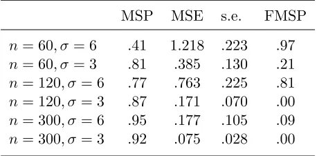
Table 4.2: Simulation results for Model 2 (t= 3) MSP MSE s.e. FMSP n= 60, σ= 6 .41 1.218 .223 .97 n= 60, σ= 3 .81 .385 .130 .21 n= 120, σ= 6 .77 .763 .225 .81 n= 120, σ= 3 .87 .171 .070 .00 n= 300, σ= 6 .95 .177 .105 .09 n= 300, σ= 3 .92 .075 .028 .00
MSP is the rate of correct model selection (treatsγ2 as 0),
In our simulations, when sample size is bigger than 120 or σ is less than 3, F-test ‘rule of thumb’ often fails to detect whether weak instruments are in the model. F-test ‘rule of thumb’ tends to miss the mark of model selection since it usually cannot reject the H0 that
both coefficients are zero. It is known that rejection of the null hypothesis by no means implies there is no weak instrument (Staiger and Stock, 1997). One issue of using of F-test is, as it is illustrated in our simulation, the researchers could not decide which instrument is weak based on the result of F-test unless they do subset selection (t test wouldn’t work) which we know is prone to instability (similar to BIC) plus size distortion. On the other hand, adaptive lasso not only shows there are weak instruments in the model, it specifically tells which ones are (by shrinking them to 0). We see as the sample size increase the correct model selection rate is getting closer to 1. Most importantly, in the case of weak instrument where the parameter is small but not zero, adaptive lasso can also estimate it as 0 in finite sample with positive probability.
4.2
Effect of Adaptive Lasso Selection V.S. Non-selection on
TSLS Estimator
Recall the original research problem of this paper is to select the strong instruments for TSLS regression. Weak instruments lead to a nonstandard distribution and bias toward plim( ˜βOLS). TSLS is consistent because it only picks up information from the strong instruments asn→ ∞. But finite sample property such as bias of IV estimator can be affected by the irrelevant in-struments. It is crucial to the study how IV selection affect the finite sample property of TSLS estimator in the aspect statistical inference. In simulation we find out that the instrumental variable selection in reduced form equation improves the inference of TSLS estimator.
We conduct the study in the following two steps. (i) Adaptive lasso selection was imple-mented in the first stage reduced form equation. (ii) Use the selected instruments in conven-tional TSLS. We report the median bias (Bias), MSE and standard error (s.e.) of the TSLS estimator for the full model (with all instruments), the strong/weak instruments only model and the adaptive lasso selected model.
The linear IV regression model with a single endogenous regressor and no included exoge-nous variable is:
yi=βxi+i (4.1)
β is the scalar parameter of interest, fix the true valueβ = 1. zi = (z1i,z2i)∼i.i.d. N(0, I2),
i = 1,2, . . . , n. The errors (i, νi) ∼ i.i.d. N(0,Σ) ( i = 1,2, . . . , n ), where Σ =
"
σ2 σν
σν σν2
#
. ρ=σν/(σσν) is correlation between the two error termsand ν. Letσ=σν =σ. The degree
of endogeneity is controlled by the covariance ρ. The closerρ is to 1, the stronger endogeneity xis. We use two values for ρ, .5 and .99. n= 60, 120, 300. Each model is replicated 500 times. We use the following three settings of γ. Notice we model weak instrument by using local to 0 (Model 4) and small but nonzero (Model 4’), the former one is more interesting in theory.
Model 3 : one strong and one irrelevant instruments. γ = (1,0)0 Model 4: one strong and one weak instruments. γ = (1,√t
n)
0, where t is a constant real number
Model 4’: one strong and one weak instruments. γ = (1, .1)0
We show in Table 4.3 and Table 4.4 that first stage adaptive lasso selection improves the accuracy and inference of TSLS estimator. We have three comparison models, (i) the full model which uses all available instruments, (ii) the model which uses only the strong instrument (SO), and (iii) the model which uses only the weak instrument (WO). The bias of adaptive lasso selected model is generally smaller than the full model which uses all available instruments. In Table 4.4 we can see the effect of instruments selection in weak instruments case. When the sample size is 300 and 1000, adaptive lasso selected IV estimator has much smaller bias than the full model.
Table 4.3: Summary statistics of TSLS for Model 3
SO WO FM AD
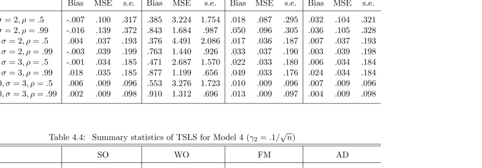
Bias MSE s.e. Bias MSE s.e. Bias MSE s.e. Bias MSE s.e. n= 60, σ= 2, ρ=.5 -.007 .100 .317 .385 3.224 1.754 .018 .087 .295 .032 .104 .321 n= 60, σ= 2, ρ=.99 -.016 .139 .372 .843 1.684 .987 .050 .096 .305 .036 .105 .328 n= 120, σ= 2, ρ=.5 .004 .037 .193 .376 4.491 2.086 .017 .036 .187 .007 .037 .193 n= 120, σ= 2, ρ=.99 -.003 .039 .199 .763 1.440 .926 .033 .037 .190 .003 .039 .198 n= 300, σ= 3, ρ=.5 -.001 .034 .185 .471 2.687 1.570 .022 .033 .180 .006 .034 .184 n= 300, σ= 3, ρ=.99 .018 .035 .185 .877 1.199 .656 .049 .033 .176 .024 .034 .184 n= 1000, σ= 3, ρ=.5 .006 .009 .096 .553 3.276 1.723 .010 .009 .096 .007 .009 .096 n= 1000, σ= 3, ρ=.99 .002 .009 .098 .910 1.312 .696 .013 .009 .097 .004 .009 .098
Table 4.4: Summary statistics of TSLS for Model 4 (γ2 =.1/ √
n)
SO WO FM AD
Bias MSE s.e. Bias MSE s.e. Bias MSE s.e. Bias MSE s.e. n= 60, σ= 2, ρ=.5 -.009 .092 .304 .433 2.736 1.596 .026 .077 .277 .026 .091 .301 n= 60, σ= 2, ρ=.99 .013 .141 .375 .802 1.324 .824 .076 .089 .288 .070 .103 .313 n= 120, σ= 2, ρ=.5 .004 .039 .199 .343 3.054 1.714 .017 .038 .193 .009 .039 .198 n= 120, σ= 2, ρ=.99 .023 .041 .202 .796 1.418 .886 .052 .038 .189 .030 .040 .198 n= 300, σ= 3, ρ=.5 -.003 .034 .184 .375 4.148 2.002 .014 .032 .179 .003 .033 .183 n= 300, σ= 3, ρ=.99 -.003 .036 .191 .881 1.507 .855 .032 .034 .180 .007 .036 .188 n= 1000, σ= 3, ρ=.5 .004 .009 .096 .418 4.199 2.006 .008 .009 .096 .004 .009 .096 n= 1000, σ= 3, ρ=.99 .006 .009 .097 .897 1.237 .657 .017 .009 .096 .007 .009 .097
Table 4.5: Summary statistics of TSLS for Model 4’
SO WO FM AD
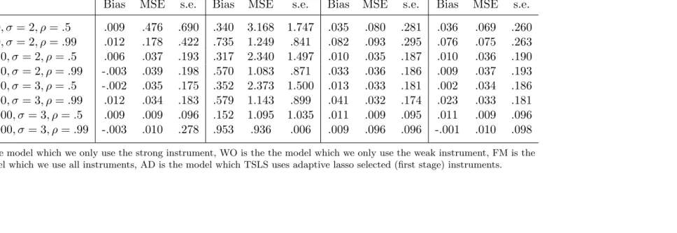
Bias MSE s.e. Bias MSE s.e. Bias MSE s.e. Bias MSE s.e. n= 60, σ= 2, ρ=.5 .009 .476 .690 .340 3.168 1.747 .035 .080 .281 .036 .069 .260 n= 60, σ= 2, ρ=.99 .012 .178 .422 .735 1.249 .841 .082 .093 .295 .076 .075 .263 n= 120, σ= 2, ρ=.5 .006 .037 .193 .317 2.340 1.497 .010 .035 .187 .010 .036 .190 n= 120, σ= 2, ρ=.99 -.003 .039 .198 .570 1.083 .871 .033 .036 .186 .009 .037 .193 n= 300, σ= 3, ρ=.5 -.002 .035 .175 .352 2.373 1.500 .013 .033 .181 .002 .034 .186 n= 300, σ= 3, ρ=.99 .012 .034 .183 .579 1.143 .899 .041 .032 .174 .023 .033 .181 n= 1000, σ= 3, ρ=.5 .009 .009 .096 .152 1.095 1.035 .011 .009 .095 .011 .009 .096 n= 1000, σ= 3, ρ=.99 -.003 .010 .278 .953 .936 .006 .009 .096 .096 -.001 .010 .098
4.3
Adaptive Lasso V.S. Donald and Newey (2001)
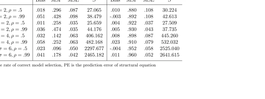
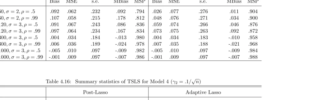
In empirical studies, DN (2001) is most commonly used method in selection of instruments. We now compare TSLS estimator using adaptive lasso with that of DN (2001) which chooses the number of instruments to minimize the leading term of Nagar (1959) type MSE. DN (2001)’s method integrates bias-variance trade-off but it does not target on correct model selection of the reduced form equation. We could improve the bias performance of TSLS using adaptive lasso, since adaptive lasso can give us the correct model. E.g., if the true reduced form equation is Model 5 below, including the irrelevant instrument could reduce the MSE, but as we know, the irrelevant instrument should not be in the model. So DN (2001) only focus on minimizing MSE, but the cost is including some weak instruments3 in the model which could aggravate the bias. We show the advantage of adaptive lasso in bias and inference given the model has both strong and weak instruments. In Table 4.6 and Table 4.7 we report the median bias, correct model selection rate, MSE and prediction error (or sampling error) of TSLS estimator over 500 replicates.
3
Table 4.6: Summary statistics for Model 3: Donald and Newey v.s. adaptive lasso Donald & Newey Adaptive Lasso
Bias MSP MSE Sˆ Bias MSP MSE Sˆ
n= 60, σ= 2, ρ=.5 .038 .320 .082 29.129 .008 .908 .107 32.731 n= 60, σ= 2, ρ=.99 .063 .524 .086 32.201 .024 .906 .101 35.912 n= 120, σ= 2, ρ=.5 .018 .312 .032 23.714 .010 .950 .033 25.321 n= 120, σ= 2, ρ=.99 .040 .546 .035 33.088 .027 .954 .042 35.960 n= 300, σ= 4, ρ=.5 .055 .152 .059 382.778 .021 .930 .081 422.198 n= 300, σ= 4, ρ=.99 .067 .288 .072 505.455 .015 .920 .086 551.779 n= 1000, σ= 6, ρ=.5 .031 .110 .038 1956.240 .016 .984 .046 2097.839 n= 1000, σ= 6, ρ=.99 .021 .192 .038 2714.484 -.011 .968 .047 2939.944
Table 4.7: Summary statistics for Model 4 (γ2=.1/ √
n): Donald and Newey v.s. adaptive lasso
Donald & Newey Adaptive Lasso
Bias MSP MSE Sˆ Bias MSP MSE Sˆ
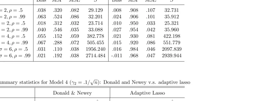
n= 60, σ= 2, ρ=.5 .048 .298 .109 24.833 .018 .876 .132 27.706 n= 60, σ= 2, ρ=.99 .038 .536 .096 35.513 .003 .888 .107 38.545 n= 120, σ= 2, ρ=.5 .040 .316 .038 26.867 .036 .950 .039 28.234 n= 120, σ= 2, ρ=.99 .040 .548 .035 33.062 .027 .954 .042 35.970 n= 300, σ= 4, ρ=.5 .055 .152 .059 380.246 .021 .922 .083 417.718 n= 300, σ= 4, ρ=.99 .066 .288 .072 505.088 .014 .922 .086 551.963 n= 1000, σ= 6, ρ=.5 .031 .104 .038 1955.731 .016 .984 .046 2097.958 n= 1000, σ= 6, ρ=.99 .035 .170 .042 2388.511 .003 .974 .047 2540.909
Table 4.8: Summary statistics for Model 4’: Donald and Newey v.s. adaptive lasso Donald & Newey Adaptive Lasso
Bias MSP MSE Sˆ Bias MSP MSE Sˆ
n= 60, σ= 2, ρ=.5 .018 .296 .087 27.065 .010 .880 .108 30.224 n= 60, σ= 2, ρ=.99 .051 .428 .098 38.479 -.003 .892 .108 42.613 n= 120, σ= 2, ρ=.5 .011 .258 .035 25.659 .004 .922 .037 27.509 n= 120, σ= 2, ρ=.99 .036 .474 .035 44.176 .005 .930 .043 37.735 n= 300, σ= 4, ρ=.5 .032 .142 .063 406.162 .008 .898 .087 445.260 n= 300, σ= 4, ρ=.99 .058 .252 .063 482.168 .023 .910 .079 532.032 n= 1000, σ= 6, ρ=.5 .023 .096 .050 2297.677 -.004 .952 .058 2525.040 n= 1000, σ= 6, ρ=.99 .041 .178 .042 2465.182 .011 .960 .052 2641.615
We now discuss briefly how the DN (2001) method work. Use the notation in (4.1) and (4.2), the 2SLS estimator is
ˆ
β= (X0PKX)−1X0PKY
where X = (x1, . . . , xn)0, Y = (y1, . . . , yn)0 and PK =ZK(ZK0ZK)−1ZK, where K is the
index for the number of instruments included in the regression. In Model 5, since we have 2 instruments, K = 1,2. And for each K, we can have different choice of instruments, e.g., Z1 = (z1,1, . . . , z1,n) or Z1 = (z2,1, . . . , z2,n), Z1 is n×1. And Z2 = (z1, . . . , zn), where
z = (z1, z2), and Z2 is n×2. As pointed out in DN (2001), ZK corresponds to a series of
instruments. But when K is large, we don’t know which instruments we should use, and it could be very computationally consuming when K gets large.
Now we define the necessary variables to minimize MSE with respect to K as described in DN (2001). Let ˜βbe some preliminary estimator ofβ, e.g., it can be the regular 2SLS estimator. ˜
=Y −Xβ. ˜˜ H =X0PKX/n. ˜u= (I−PK)X. ˜uλ = ˜uH˜−1˜λ, where we let ˜λ= 1 (see details
in DN 2001). We have the following variables: ˆσ2 = ˜0˜/n, ˆσλ2 = ˜u0λu˜λ/n, ˆσλ= ˜u0λ/n. These˜
preliminary estimators are not depend on K, they remain as constants as the approximate of MSE for different instruments are calculated. Define a Mallow’s creteria. First, let ˆuK = (I −PK)X, ˆuKλ = ˆuKH˜λ. So the Mallow’s creteria is ˆˆ Rmλ(K) = uˆ
K λ0uˆKλ
n + ˆσ
2
λ(2K/n). Finally,
the approximate MSE of the 2SLS estimator is ˆSλ(K) = ˆσ2λ
K2 n + ˆσ
2
ˆ
Rmλ(K)−σλ2K n
. Table 4.6 and 4.7 show that DN (2001) TSLS estimator has smaller MSE but higher bias than that of adaptive lasso. We can also see that DN (2001) performs sub par in model selection. This is an evidence that only minimizing MSE does not guarantee consistent model selection. So in the aspect of using the correct model in TSLS, adaptive lasso is better. In the case of identifiable model with both strong and weak instruments, adaptive lasso gives us asymptotic efficiency on TSLS estimator. Also notice that bias and MSE is higher as the degree of endogeneity increases.
4.4
Adaptive Lasso V.S. Model Averaging
KO (2010)4 and DN (2001). For comparison of adaptive lasso and DN (2001), we also report correct model selection rate (MSP) and the MSE as defined in DN (2001)5. Table 4.9 to 4.14 report the results based on 500 repeats.
We use the following two setup ofγ :
Model 5 : one nonzero (strong) and one exact zero coefficientsγ = (.8,0)0
Model 6: one nonzero (strong) and one local to zero (weak) coefficients γ = (.8,√t
n)
0
, wheret is a constant real number
4
We report the minimum MSE of KO (2010) among the restrictions U, C, P, Ps.
Table 4.9: Summary statistics for Model 5 (ρ=.1): Model averaging v.s. adaptive lasso Adaptive Lasso Donald & Newey Model Averaging
Bias MSP MSE Sˆ Bias MSP MSE Sˆ Bias MSE
n= 60, σ= 1.5 -.010 .916 .083 22.678 -.008 .690 .071 22.642 -.005 .069 n= 120, σ= 1.5 .001 .952 .032 18.779 .004 .722 .031 18.752 .006 .031 n= 300, σ= 3 -.011 .956 .063 279.272 -.001 .706 .052 279.073 -.001 .052 n= 300, σ= 1.5 .003 .980 .011 13.632 .004 .726 .011 13.620 .003 .011 n= 500, σ= 3 .010 .992 .032 267.588 .009 .698 .033 267.428 .010 .032 n= 1000, σ= 3 .007 .990 .015 222.888 .008 .654 .014 222.795 .009 .015
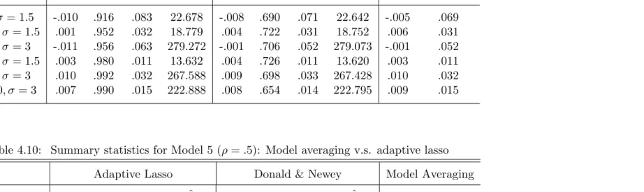
Table 4.10: Summary statistics for Model 5 (ρ=.5): Model averaging v.s. adaptive lasso Adaptive Lasso Donald & Newey Model Averaging
Bias MSP MSE Sˆ Bias MSP MSE Sˆ Bias MSE
n= 60, σ= 1.5 .019 .908 .078 21.651 .033 .750 .073 21.611 .038 .067 n= 120, σ= 1.5 .010 .944 .037 18.601 .017 .742 .034 18.579 .022 .033 n= 300, σ= 3 -.001 .970 .071 337.072 .010 .720 .069 336.861 .025 .062 n= 300, σ= 1.5 .004 .962 .012 14.810 .007 .748 .012 14.799 .011 .011 n= 500, σ= 3 .004 .970 .031 303.306 .018 .716 .030 303.169 .022 .029 n= 1000, σ= 3 .006 .984 .014 228.485 .012 .700 .013 228.399 .013 .013
Table 4.11: Summary statistics for Model 5 (ρ=.9): Model averaging v.s. adaptive lasso Adaptive Lasso Donald & Newey Model Averaging
Bias MSP MSE Sˆ Bias MSP MSE Sˆ Bias MSE
n= 60, σ= 1.5 .016 .888 .093 25.174 .033 .790 .129 25.151 .071 .095 n= 120, σ= 1.5 -.006 .962 .036 22.865 .004 .844 .034 22.845 .021 .032 n= 300, σ= 3 .003 .944 .078 346.590 .022 .698 .062 346.418 .041 .052 n= 300, σ= 1.5 .009 .976 .013 14.950 .020 .798 .012 14.939 .026 .012 n= 500, σ= 3 .010 .982 .039 351.957 .028 .744 .034 351.792 .035 .032 n= 1000, σ= 3 .014 .986 .015 245.571 .020 .748 .014 245.513 .026 .014
Table 4.12: Summary statistics for Model 6 (ρ=.1): Model averaging v.s. adaptive lasso Adaptive Lasso Donald & Newey Model Averaging
Bias MSP MSE Sˆ Bias MSP MSE Sˆ Bias MSE
n= 60, σ= 1.5 -.020 .918 .085 22.013 -.020 .674 .074 21.960 -.020 .073 n= 120, σ= 1.5 .010 .966 .033 17.656 .009 .702 .032 17.629 .009 .031 n= 300, σ= 3 -.009 .954 .067 267.702 .006 .686 .048 267.471 .003 .047 n= 300, σ= 1.5 .005 .982 .012 13.944 .006 .684 .012 13.929 .006 .012 n= 500, σ= 3 .002 .982 .029 250.872 .003 .666 .029 250.704 .004 .028 n= 1000, σ= 3 -.001 .988 .014 235.262 -.001 .732 .014 235.187 -.003 .014
Table 4.13: Summary statistics for Model 6 (ρ=.5): Model averaging v.s. adaptive lasso Adaptive Lasso Donald & Newey Model Averaging
Bias MSP MSE Sˆ Bias MSP MSE Sˆ Bias MSE
n= 60, σ= 1.5 .003 .904 .095 21.767 .020 .752 .082 21.734 .037 .076 n= 120, σ= 1.5 -.007 .930 .035 22.116 .001 .742 .034 22.089 .003 .032 n= 300, σ= 3 .010 .960 .063 310.169 .028 .672 .059 309.944 .034 .055 n= 300, σ= 1.5 -.004 .978 .012 14.975 .001 .744 .012 14.960 .001 .012 n= 500, σ= 3 .001 .968 .029 273.088 .016 .676 .028 272.935 .024 .028 n= 1000, σ= 3 .012 .988 .015 231.736 .014 .734 .014 231.672 .019 .014
Table 4.14: Summary statistics for Model 6 (ρ=.9): Model averaging v.s. adaptive lasso Adaptive Lasso Donald & Newey Model Averaging
Bias MSP MSE Sˆ Bias MSP MSE Sˆ Bias MSE
n= 60, σ= 1.5 .029 .900 .095 28.392 .044 .812 .097 28.372 .072 .080 n= 120, σ= 1.5 .006 .968 .038 24.444 .014 .838 .037 24.430 .033 .033 n= 300, σ= 3 .023 .938 .068 387.483 .041 .738 .064 387.314 .063 .057 n= 300, σ= 1.5 -.003 .978 .014 15.870 .006 .786 .013 15.857 .009 .012 n= 500, σ= 3 -.007 .988 .036 366.645 .005 .766 .034 366.516 .019 .032 n= 1000, σ= 3 .014 .988 .016 239.523 .020 .718 .015 239.446 .025 .015
In both Model 5 and Model 6, KO (2010) weighted TSLS estimator has the least regular MSE among the three methods. Adaptive lasso selected TSLS estimator has greatest MSE among the three methods. Also adaptive lasso selected TSLS estimator has higher DN type MSE than DN (2001) selected TSLS estimator. When endogeneity is weak,ρ=.1, the adaptive lasso selected TSLS is outperformed by both DN (2001) and KO (2010) in bias and MSE in small sample sizes. For ρ=.5 and ρ =.9, adaptive lasso selected TSLS estimator has much smaller bias than both DN (2001) and KO (2010) most of the time (except for Model 6, n = 300, σ = 1.5). As the degree of endogeneity (ρ) increase, the bias of the three TSLS estimators increase compared to collateral group. For DN (2001) and KO (2010), bias decreases as the sample size increases. Adaptive lasso model selection is converging when sample size increases, but DN (2001) does not.
4.5
Adaptive Lasso V.S. Post-Lasso
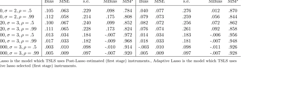
In this section we compare the performance of TSLS estimator by adaptive lasso selection with the one by Post-Lasso estimation of IVs (using Algorithm 2.2 of Belloni et al. (2010)). To estimate the optimal IV set in their method, lasso procedure selects the relevant instruments first. We use Model 3, Model 4 and Model 4’ as the DGP. Using Model 3 as an example, post-lasso is a method that estimates instrument set (and more generally, conditional expectation functions), wherez= (z1, z2), such thatD(z) =E(x|z). The post-lasso procedure doesn’t rely
on model selection of relevant z’s directly, but the selected z plays important role of predict D(z). As showed in Caner and Fan (2011), adaptive lasso is consistent in model selection while
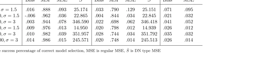
lasso is not. From Table 4.15 we see that when the sample size is small and variance is relatively large, adaptive lasso selected TSLS method has smaller bias. When sample size is large, the two methods are similar and both are consistent. We also show the simulation results using BIC tuning and optimal inequality tuning parameterλ.
Table 4.15: Summary statistics of TSLS for Model 3
Post-Lasso Adaptive Lasso
Bias MSE s.e. MBias MSP Bias MSE s.e. MBias MSP
n= 60, σ= 2, ρ=.5 .092 .062 .232 .092 .794 .026 .077 .276 .011 .904 n= 60, σ= 2, ρ=.99 .107 .058 .215 .178 .812 .048 .076 .271 .034 .900 n= 120, σ= 3, ρ=.5 .091 .067 .243 .086 .836 .059 .074 .266 .046 .876 n= 120, σ= 3, ρ=.99 .097 .064 .234 .167 .834 .073 .075 .263 .092 .872 n= 300, σ= 3, ρ=.5 .004 .034 .184 -.013 .980 .004 .034 .183 -.010 .958 n= 300, σ= 3, ρ=.99 .006 .036 .189 -.024 .978 .007 .035 .188 -.021 .968 n= 1000, σ= 3, ρ=.5 -.005 .010 .097 -.009 .982 -.005 .010 .097 -.009 .984 n= 1000, σ= 3, ρ=.99 -.001 .009 .097 -.007 .986 -.001 .009 .097 -.007 .988
Table 4.16: Summary statistics of TSLS for Model 4 (γ2 =.1/ √
n)
Post-Lasso Adaptive Lasso
Bias MSE s.e. MBias MSP Bias MSE s.e. MBias MSP
n= 60, σ= 2, ρ=.5 .083 .062 .234 .088 .830 .032 .076 .274 .011 .898 n= 60, σ= 2, ρ=.99 .102 .059 .221 .164 .822 .054 .076 .270 .038 .878 n= 120, σ= 3, ρ=.5 .077 .066 .245 .073 .832 .060 .073 .263 .042 .844 n= 120, σ= 3, ρ=.99 .106 .065 .231 .157 .854 .075 .070 .255 .093 .874 n= 300, σ= 3, ρ=.5 .005 .034 .184 -.025 .990 .005 .034 .183 -.024 .974 n= 300, σ= 3, ρ=.99 -.007 .038 .194 -.038 .984 -.006 .038 .195 -.039 .974 n= 1000, σ= 3, ρ=.5 -.005 .010 .098 -.006 .992 -.005 .010 .098 -.006 .996 n= 1000, σ= 3, ρ=.99 .004 .009 .097 -.006 .982 .004 .009 .097 -.006 .980
Table 4.17: Summary statistics of TSLS for Model 4’
Post-Lasso Adaptive Lasso
Bias MSE s.e. MBias MSP Bias MSE s.e. MBias MSP
n= 60, σ= 2, ρ=.5 .105 .063 .229 .098 .784 .040 .077 .276 .012 .870 n= 60, σ= 2, ρ=.99 .112 .058 .214 .175 .808 .079 .073 .259 .056 .844 n= 120, σ= 3, ρ=.5 .100 .067 .240 .099 .852 .082 .072 .256 .072 .862 n= 120, σ= 3, ρ=.99 .111 .065 .228 .173 .824 .076 .074 .261 .092 .858 n= 300, σ= 3, ρ=.5 .013 .034 .184 -.007 .972 .014 .034 .183 -.006 .956 n= 300, σ= 3, ρ=.99 .017 .033 .182 -.009 .968 .018 .033 .181 -.007 .948 n= 1000, σ= 3, ρ=.5 .003 .010 .098 -.010 .914 -.003 .010 .098 -.011 .926 n= 1000, σ= 3, ρ=.99 .005 .009 .097 -.007 .920 .005 .009 .097 -.007 .928
Table 4.18: Summary statistics of TSLS for Model 3
Post-Lasso Adaptive Lasso (λ)
Bias MSE s.e. MBias MSP Bias MSE s.e. MBias MSP
n= 60, σ= 2, ρ=.5 .093 .062 .232 .094 .794 .090 .062 .231 .087 .826 n= 60, σ= 2, ρ=.99 .122 .060 .212 .188 .804 .117 .058 .210 .182 .832 n= 120, σ= 3, ρ=.5 .101 .068 .240 .095 .836 .182 .073 .200 .169 .714 n= 120, σ= 3, ρ=.99 .117 .064 .225 .183 .830 .174 .061 .174 .320 .726 n= 300, σ= 3, ρ=.5 .015 .035 .186 -.008 .980 .015 .034 .183 -.003 .990 n= 300, σ= 3, ρ=.99 .015 .035 .187 -.020 .978 .012 .034 .185 -.014 .992 n= 1000, σ= 3, ρ=.5 -.002 .009 .097 -.001 .990 -.003 .009 .097 -.001 1.000 n= 1000, σ= 3, ρ=.99 .004 .009 .096 -.003 .976 .004 .009 .097 -.004 1.000
Table 4.19: Summary statistics of TSLS for Model 4 (γ2 =.1/ √
n)
Post-Lasso Adaptive Lasso (λ)
Bias MSE s.e. MBias MSP Bias MSE s.e. MBias MSP
n= 60, σ= 2, ρ=.5 .072 .061 .236 .070 .834 .076 .059 .231 .079 .842 n= 60, σ= 2, ρ=.99 .109 .061 .222 .172 .796 .110 .058 .214 .188 .806 n= 120, σ= 3, ρ=.5 .081 .062 .236 .093 .808 .148 .062 .201 .155 .708 n= 120, σ= 3, ρ=.99 .111 .063 .225 .187 .818 .183 .062 .171 .336 .700 n= 300, σ= 3, ρ=.5 .008 .033 .182 -.011 .986 .008 .033 .180 -.006 .994 n= 300, σ= 3, ρ=.99 -.004 .036 .190 -.030 .976 -.009 .036 .190 -.029 .996 n= 1000, σ= 3, ρ=.5 .001 .009 .097 -.004 .982 -.001 .009 .097 -.004 1.000 n= 1000, σ= 3, ρ=.99 .003 .009 .096 -.003 .990 .002 .009 .097 -.004 .998
Table 4.20: Summary statistics of TSLS for Model 4’
Post-Lasso Adaptive Lasso (λ)
Bias MSE s.e. MBias MSP Bias MSE s.e. MBias MSP
n= 60, σ= 2, ρ=.5 .087 .061 .232 .080 .822 .096 .061 .227 .092 .824 n= 60, σ= 2, ρ=.99 .102 .058 .219 .173 .802 .115 .054 .202 .211 .784 n= 120, σ= 3, ρ=.5 .085 .068 .247 .080 .832 .160 .065 .198 .172 .700 n= 120, σ= 3, ρ=.99 .108 .065 .231 .166 .834 .176 .062 .175 .317 .726 n= 300, σ= 3, ρ=.5 -.013 .034 .184 -.015 .956 -.015 .034 .183 -.014 .992 n= 300, σ= 3, ρ=.99 .013 .034 .185 -.014 .954 .008 .033 .182 -.005 .982 n= 1000, σ= 3, ρ=.5 .002 .009 .096 -.002 .908 -.001 .009 .097 -.004 .992 n= 1000, σ= 3, ρ=.99 .002 .010 .098 -.009 .912 -.001 .010 .098 -.012 .994
Table 4.21: Correct Model Selection Percentage for Just Identified Model (One weak.1/√n) Post Lasso Adaptive Lasso (BIC) Adaptive Lasso (λ)
n= 60, σ= 2, ρ=.5 .988 .944 .992
n= 60, σ= 2, ρ=.99 .988 .960 .994
n= 60, σ= 3, ρ=.5 .980 .956 .986
n= 60, σ= 3, ρ=.99 .990 .958 .996
n= 120, σ= 3, ρ=.5 .994 .986 .998
n= 120, σ= 3, ρ=.99 .974 .948 .996
n= 300, σ= 3, ρ=.5 .992 .984 1.000
n= 300, σ= 3, ρ=.99 .986 .988 .998
n= 1000, σ= 3, ρ=.5 .976 .984 1.000
n= 1000, σ= 3, ρ=.99 .982 .992 1.000
Adaptive Lasso (BIC), Adaptive Lasso (λ) are adaptive lasso using BIC and optimal inequalityλtuning methods respectively.
4.6
Adaptive Lasso V.S. AIC and BIC
In this section we compare TSLS performance of adaptive lasso with that of AIC and BIC model selection. The model we use is
yi =βxi+i (4.3)
xi =ziγ+νi (4.4)
where zi = [z1i z2i . . . z9i], γ = (γ1 γ2. . . γ9)T. The model setup is the same as (4.1)
and (4.2) except that the dimension of γ is 9 and the distribution of zi is now N(0,Σz). Let
Q=
1 0 . . . 0
1
√
2 1
√
2 . . . 0
.. . ... . .. ... 1 √ 9 1 √
9 . . . 1 √ 9
a triangular matrix. Qij = √1i, fori≥j and Qij = 0, for i < j.
Σz =QTQ. The true value ofγ is:
Model 7: four nonzero (strong) and five exact zero coefficientsγ = (1,0, .8,0, .7,0,0,0, .9)0 Model 8: four nonzero (strong) and five exact zero coefficientsγ = (1,√t
n, .8, t
√
n, .7, t √ n, t √ n, t √
n, .9)
0
, wheret is a constant real number
Model 8’: four nonzero (strong) and five exact zero coefficientsγ = (1, .1, .8, .1, .7, .1, .1, .1, .9)0, wheret is a constant real number
Table 4.22: Summary statistics for Model 7: AIC / BIC v.s. adaptive lasso
AIC BIC Adaptive Lasso
Bias MSP MSE Bias MSP MSE Bias MSP MSE
n= 60, σ= 1.5, ρ=.5 .024 .10 .004 .025 .07 .004 .017 .14 .004 n= 60, σ= 1.5, ρ=.99 .029 .11 .005 .023 .06 .005 .023 .16 .005 n= 120, σ= 1.5, ρ=.5 .017 .29 .002 .016 .32 .002 .015 .36 .002 n= 120, σ= 1.5, ρ=.99 .007 .29 .002 .005 .28 .002 .004 .39 .002 n= 300, σ= 3, ρ=.5 .023 .17 .005 .023 .01 .005 .021 .24 .005 n= 300, σ= 3, ρ=.99 .036 .16 .003 .030 .03 .003 .029 .22 .003 n= 300, σ= 1.5, ρ=.5 .006 .48 .001 .006 .77 .001 .006 .72 .001 n= 300, σ= 1.5, ρ=.99 .010 .44 .001 .010 .75 .001 .010 .67 .001 n= 500, σ= 3, ρ=.5 .013 .29 .002 .012 .25 .002 .011 .36 .002 n= 500, σ= 3, ρ=.99 .012 .29 .002 .012 .18 .002 .009 .35 .002 n= 500, σ= 1.5, ρ=.5 .006 .52 .001 .005 .91 .001 .005 .86 .001 n= 500, σ= 1.5, ρ=.99 .001 .43 .001 .001 .89 .001 .001 .82 .001 n= 1000, σ= 1.5, ρ=.5 .001 .46 .001 .001 .96 .001 .001 .90 .002 n= 1000, σ= 1.5, ρ=.99 .001 .49 .001 -.001 .97 .001 -.001 .93 .001
Table 4.23: Summary statistics for Model 8 (t=.1): AIC / BIC v.s. adaptive lasso
AIC BIC Adaptive Lasso
Bias MSP MSE Bias MSP MSE Bias MSP MSE
n= 60, σ= 1.5, ρ=.5 .025 .11 .005 .027 .04 .005 .023 .16 .005 n= 60, σ= 1.5, ρ=.99 .019 .06 .003 .015 .09 .003 .015 .16 .003 n= 120, σ= 1.5, ρ=.5 .005 .33 .002 .007 .28 .002 .002 .39 .002 n= 120, σ= 1.5, ρ=.99 .023 .22 .003 .021 .24 .003 .020 .31 .003 n= 300, σ= 3, ρ=.5 .023 .17 .005 .022 .01 .005 .021 .24 .005 n= 300, σ= 3, ρ=.99 .033 .16 .003 .030 .05 .003 .029 .22 .003 n= 300, σ= 1.5, ρ=.5 .002 .41 .001 .001 .75 .001 .001 .68 .001 n= 300, σ= 1.5, ρ=.99 .002 .40 .001 .002 .74 .001 .002 .65 .001 n= 500, σ= 3, ρ=.5 .009 .29 .002 .007 .21 .002 .007 .33 .002 n= 500, σ= 3, ρ=.99 .025 .28 .002 .024 .29 .002 .022 .34 .002 n= 500, σ= 1.5, ρ=.5 .003 .45 .001 .003 .87 .001 .003 .77 .001 n= 500, σ= 1.5, ρ=.99 .003 .40 .001 .002 .88 .001 .001 .76 .001 n= 1000, σ= 1.5, ρ=.5 .003 .47 .001 .003 .98 .001 .003 .94 .001 n= 1000, σ= 1.5, ρ=.99 .001 .40 .001 -.001 .97 .001 -.001 .94 .001
4.7
Adaptive Lasso and Best Subset Selection
The advantage of adaptive lasso compared to other traditional model selection method such as best subset selection using AIC/BIC is of threefold. First, when the number of variables is large, the computation of subset selection becomes infeasible. Second, subset selection is instable because of its discreteness (Breiman 1995). Small changes in the data can result in very different model selection. Third, step wise selection ignores stochastic errors in the variable selection process. We illustrate this problem and compare the model performance of adaptive lasso and best subset selection using a simple example. In the reduced form equation (4.4), zi∼N(0,Σz). Qij = √1i, fori≥j and Qij = 0, for i < j. Σz=QTQ, we have true value of
Model 9 : γ = (1,0, .7,0, .9,0,0,0) Model 10 : γ = (1,√t
n, .7, t
√
n, .9, t
√
n, t
√
n, t
√
n)
Table 4.24 and Table 4.25 show the result. In small samples adaptive lasso has significant advantage over BIC. If we increase the sample size to 1000, BIC is not dominated by adaptive lasso, since both are consistent method.
Table 4.24: Success rate of model selection: Model 9 BIC Adaptive Lasso
n= 60, σ= 1.5 .15 .30
n= 120, σ= 1.5 .41 .52
n= 300, σ= 1.5 .84 .85
n= 1000, σ= 1.5 .98 .98
Table 4.25: Success rate of model selection: Model 10 BIC Adaptive Lasso
n= 60, σ= 1.5 .08 .20
n= 120, σ= 1.5 .76 .64
n= 300, σ= 1.5 .93 .86
n= 1000, σ= 1.5 .95 .93
Chapter 5
Returns to Education Revisited
We attempt to give a theoretical guideline for instruments selection by adaptive lasso in previous chapters. Our Monte Carlo study shows that adaptive lasso method performs better compared to other existing methods in the perspective of reducing finite sample bias and correct model selection. It is very important to point out that our method is computationally efficient so that empirical researcher would find that adaptive lasso first stage selection is easy to implement. It is thus necessary to study the instruments selection problem in a real data set as a demonstration of how our method works. In this chapter we replicate and compare the adaptive lasso method with the celebrated empirical study of returns to education by Angrist and Krueger (1991) (Hereafter referred to as AK 1991). We make important contribution to the empirical results by improving the bias term.
Let us briefly introduce the research question raised by AK 1991. One important question in labor economics is that, will one extra year of compulsory education increase the wage of a worker? School education is one of the crucial factors for human capital accumulation, which will in turn improve the labor’s performance at work. There are many other forms of human capital accumulation which are heterogeneous, such as professional training (non-degree) and learning by doing. But some of these activities are not recorded in the survey questions such as the U.S. census data. Therefore one common problem in the study of returns to education is that the variable ‘years of education’ could be endogenous due to the correlation of education level and missing variable ‘ability’ in the error term. In AK 1991, quarter of birth is employed as pivotal instrumental variable which is manipulated to create more instruments. Also in AK 1991, year of birth dummy variables along with the interaction terms are used in the TSLS regression. Our ‘instruments pool’ is the full instruments set used in AK 1991. So we do not create any more instruments than the original paper.
interaction terms). In empirical studies, it is a common theme that there is no clear boundary of instruments set other than using the F-test for ‘all or none’ decision (as we show in Chapter 4, it does not work). We apply adaptive lasso method to select the instruments for years of education in the first stage. In the second stage, we include only the selected instruments. We compare the TSLS results using all instruments and the selected instruments as reported in Table 5.1.
First, we briefly describe the model and data of AK 1991. To control for the endogeneity and time trend, they use the following TSLS model:
lnWi =Xiβ+ ΣcYicξc+ρEi+µi (5.1)
Ei =Xiπ+ ΣcYicδc+ ΣcΣjYicQijθjc+i (5.2)
In the structural equation, the dependent variable lnW is the log of weekly wage. X is the vector of covariates which includes race, marital status, region of residence (SMSA), age, square of age, etc. Y is the year of birth dummy variable. The variable of interests is years of education E. Quarter of birth (Q) and year of birth (Y) dummy variables (and interaction terms) are used as instruments 6. The sample was drawn from 1980 U.S. Census data. In this replicate we use the cohort of 329,509 men whose birth year is between 1930 and 1939. We use the same variables and data as in AK 1991 Table V. And we will do adaptive lasso model selection in the first stage. We report the TSLS estimate with ‘all instruments’ as in AK 1991 Table V and the adaptive lasso selected instruments in Table 5.1. We interpret the coefficient of years of education ˆβ as following. If the representative individual increases the years of education by one more year, she would expect to have an increase (decrease if negative
ˆ
β) of wage by 100×βˆ%. For example in column 6 of Table 5.1, if the representative worker has one more year of education, her expected wage will increase by 6.65%.
Table 5.1 contains the TSLS estimate of years of education and other included exogenous variables. For each structural model setup (different included exogenous variables as shown in the very left column), we report the original TSLS estimate of AK 1991 (in odd columns) and the adaptive lasso selected TSLS (in even columns adjacent to the AK 1991 estimate). From the last row of Table 5.1 we see that adaptive lasso method always selects a subset of the instruments set. This result implies that each full model (with all instruments) has unwanted instruments. In our first stage adaptive lasso estimation, year of birth dummy variables are in most of the selected sets. But some year and quarter of birth interaction terms are not selected (shrunk to zero by adaptive lasso). These instruments that we throw out may satisfy the orthogonality condition but they are not correlated with the endogenous variable hence they are very weak. By doing adaptive lasso shrinkage, we are able to get a desired parsimonious
6
model with less ‘noise’ from many junk instruments. This is important for finite sample bias term especially when the instruments set is large and sparse such as the one used in AK 1991. Therefore our method can give us the guideline in empirical studies that which instrument is strong and which one is weak. In table 5.1, the TSLS estimates are similar except for columns 5 and 6. The adaptive lasso TSLS estimate in column 6 is much smaller than the original estimate and less significant. This result gives us another angle to look at the effect of years of education. It is also clearly shown in the first row of the table, the adaptive lasso TSLS estimator is different from the AK 1991. The difference is due to finite sample properties and different instrument set.
Another concern of this study is that quarter of birth is a weak instrument (Bound et. al, 1995). The conventional asymptotic properties of TSLS will not hold under this scenario. Confidence intervals will have distorted coverage of the true coefficient. We compare adaptive lasso and conditional likelihood ratio (CLR) confidence interval reported in Table 3 of Cruz and Moreira (2005). In that paper they emphasize on the weak IV problem. It is likely that quarter of birth itself is exogenous, but it is very weakly correlated to years of education. Therefore all the instruments that are created using this instrument might also be weak. Cruz and Moreira (2005) suggests using first stage F-test as an indicator of the strength of instruments. If the instruments were very weak, more powerful test such as conditional likelihood ratio or Wald should be reported to give the correct confidence interval. We also think weak IV is a realistic problem in this case, so it might be a good id