Mathematical modelling in river pollution control

(1)

MATHEMATICAL MODELLING IN RIVER POLLUTION CONTROL

DARREL WEE CHIA KEE

(2)

MATHEMATICAL MODELLING IN RIVER POLLUTION CONTROL

DARREL WEE CHIA KEE

A thesis submitted in partial fulfillment of the requirements for the award of degree of Master of Science (Engineering Mathematics).

Faculty of Science Universiti Teknologi Malaysia

(3)

iii

My utmost dedication to Mum and Dad. Thank you for always being there for me.

(4)

iv

ACKNOWLEDGEMENT

I am indebted to my supervisor, Associate Professor Dr. Shamsuddin Ahmad for guiding me throughout this research. Through his valuable support and advices, I was able to conduct my research without encountering difficulties. His efforts have proved to be very useful when I was able to finally complete this research.

I would also like to extend my gratitude to my family members, mainly my father and mother. They have been an indispensable source of encouragement and motivation. Without them, I would not have the chance to conduct this research. Besides that, I would also like to take this opportunity to thank Miss Kee Boon Lee who has helped me in this research.

(5)

v

ABSTRACT

(6)

vi

ABSTRAK

(7)

vii

TABLE OF CONTENTS

CHAPTER TITLE PAGE

TITLE PAGE i

DECLARATION ii

DEDICATION iii

ACKNOWLEDGEMENT iv

ABSTRACT v

ABSTRAK vi

TABLE OF CONTENTS vii

LIST OF TABLES xi

LIST OF FIGURES xii

LIST OF APPENDICES xv

LIST OF SYMBOLS xvi

1 INTRODUCTION 1

1.1 Background of the Study 1

1.2 Statement of the Problem 3

1.3 Objectives of the Study 4

1.4 Scope of the Study 4

1.5 Significance of the Study 5

(8)

viii

2 LITERATURE REVIEW 7

2.1 Introduction 7

2.2 Modelling Fecal Coliform Bacteria – Model Development and Application

7

2.3 A Review on Optimal Location for Sampling Points 8

2.4 Water Quality Monitoring of Maong River, Malaysia

9

2.5 2.6

Introduction to Flow Simulation Mathematics of Transport Phenomena 2.6.1 Conservation Principles

2.6.2 Convective and Diffusive Fluxes 2.6.3 The Generic Transport Equation 2.6.4 Initial and Boundary Conditions

2.6.5 Elliptic Transport Equations 2.6.6 Hyperbolic Transport Equations 2.6.7 Parabolic Transport Equations 2.6.8 Summary of Model Problems

12 13 13 15 17 18 19 20 22 23

3 RESEARCH METHODOLOGY 25

3.1 Introduction 25

3.2 Model Design 25

3.3 Linear Advection Equation

3.3.1 Analytical Solution of the Linear Advection

Equation

3.3.2 Numerical Solution of the Linear Advection

Equation

3.3.3 First Order Upwind (FOU) Scheme

28 29

31

34 3.4 Linear Advection Equation with Decay Term

(9)

ix

Equation with Decay Term

3.4.2 Numerical Solution of the Linear Advection Equation

38

41 3.5 Linear Advection Equation with Decay and

Constant Source Term

3.5.1 Analytical Solution of the Linear Advection Equation with Decay and Constant Source Term

3.5.2 Numerical Solution of the Linear Advection Equation with Decay and Constant Source Term

41

42

43

45 3.6 Convection Reaction Equation

3.6.1 Properties of the Dirac Delta Function

3.6.2 Analytical Solution of the Convection Reaction Equation

46 47

49

4 RESULTS AND DISCUSSION 54

4.1 Introduction 54

4.2 Output for Linear Advection Equation 55

4.3 Output for Linear Advection Equation with Decay Term

58

4.4 Output for Linear Advection Equation with Decay and Constant Source Term

61

(10)

x

5 CONCLUSION AND RECOMMENDATION 70

5.1 Introduction 70

5.2 Conclusion 70

5.3 Recommendation 72

(11)

xi

LISTS OF TABLES

TABLE NO. TITLE PAGE

2.1 Summary of the models for the elliptic, hyperbolic and parabolic PDE types.

(12)

xii

LISTS OF FIGURES

FIGURE NO. TITLE PAGE

1.1 Fecal coliform bacteria. 2

2.1 Relationships of flow and water quality simulation.

11

2.2 A fixed control volume V bounded by the control surface S.

14

3.1 General Diagram of a River. 26

3.2 Initial concentration profile. 30

3.3 Concentration profile after time t (solid)

compared to initial profile (dashed), v>0.

31

3.4 Stencil of the first order upwind scheme. 36

3.5 The δ

( )

x function at x=0. 47

(13)

xiii

4.1 Solution at time, t =0s. 56

4.2 Solution at time, t=3s. 56

(14)

xiv

4.13 3D plot for time t =0 till t =10s. 65

4.14 3D plot for time t =0 till t =100s. 65

4.15 2D plot for time t=0s. 66

4.16 2D plot for time t=12.5s. 66

(15)

xv

LISTS OF APPENDICES

APPENDIX TITLE PAGE

A MATLAB Code: Linear Advection Equation. 75

B MATLAB Code: Linear Advection Equation with Decay Term.

77

C MATLAB Code: Linear Advection Equation with Decay and Constant Source Term.

79

(16)

xvi

LISTS OF SYMBOLS

A - Area of section occupied by water

j

e - Point where the j-th wastewater

discharge is located

f - Flux function

H - Height of the water

( )

x

H - Heaviside step function

0

I - Surface light energy

k - Loss rate for total coliform bacteria

1

k - Mortality rate

e

k - Extinction coefficient

i

k - Bacterial loss caused by the effect of light

s

k - Settling loss rate

( )

t

mj - Mass coliform flow rate at the j-th

wastewater discharge

s

P - Sea water’s percentage

( )

x t

u , - Coliform concentration

v - Average velocity in the river

β - Proportionality constant close to unity

(

x−b

)

δ - Dirac measure at point b

( )

t

Lx ∆ - Differential marching operator

θ - Temperature

(17)

CHAPTER 1

INTRODUCTION

1.1 Background of the Study

Since the beginning of time, people have always used rivers as garbage

disposal sites. Due to the rapid development of industries and populations,

wastewater discharges in our rivers have increased at a rapid rate. As the problem of

water pollution becomes more chronic, various developed countries have created

stringent laws concerning wastewater disposal in rivers.

Wastewater in river can be classified into two types, which are domestic

wastewater and industrial wastewater. Domestic wastewater refers to wastewater

which comes from a purifying plant where water is collected from a sewer system.

On the other hand, industrial wastewater refers to wastewater which comes from an

industrial plant.

By choosing the proper indicators of pollution levels and designing a

sampling technique which gives us the value of these indicators along the river, we

are able to ensure that the river is absorbing the discharges. To control pollution

caused by pathogenic microorganisms coming from domestic wastewater, one of the

best indicators is the concentration (units m-3) of the fecal coliform bacteria, due to

the fact that its concentration in wastewater discharges is much more compared to the

(18)

2

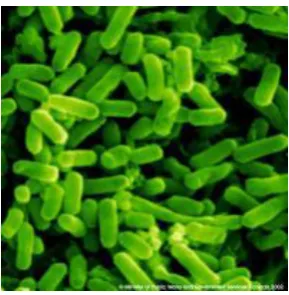
Fecal coliform bacteria are commonly found in faeces, or waste. They belong

to a larger group of organisms known as coliform bacteria. In Standard Methods for

the Examination of Water and Wastewater, 19th Edition, coliform bacteria are

classified as facultative anaerobes, which also mean that they can survive without

oxygen and are rod-shaped bacteria that produce lactose, a type of sugar.

Figure 1.1: Fecal Coliform Bacteria

Fecal coliform bacteria can originate from various sources and it depends on

the hydrologic conditions. The two main sources from which fecal coliform bacteria

originate from are human sources and non-human sources.

Human sources can be divided into two categories, sewered watersheds and

non-sewered watersheds. Sewered watersheds sources can be associated with

combined sewer overflows, sanitary sewer overflows, illegal sanitary connections to

storm drains, illegal disposal to storm drains and leaking sewer lines. Meanwhile,

non-sewered watersheds can be related to failing septic systems, small,

self-contained sewage-treatment systems and marinas and pumpout facilities.

On the other hand, non-human sources can also be split into two categories,

which are domestic animals and urban wildlife, and livestock and rural wildlife.

Dogs, cats, rats, pigeons and ducks are categorised in the domestic animals and urban

wildlife section, whereas cattle, horse, poultry and deer are categorised in the

(19)

3

To control the concentration of coliform bacteria in rivers, we can divide the

river into several sections with respect to the morphology of the river basin and the

number, type and location of the discharges, and to obtain samples of water at each

particular point of each section. The point at where the sampling station is located,

also known as sampling point, is very important if we are looking for information

about the pollution in the whole section of the river. (Alvarez-Vazquez L.J., Martinez

A., Vazquez-Mendez M.E., Vilar M., 2006)

Thus, a further study on the mathematical model development for the

transport of coliform bacteria along a river section is to be conducted. By using this

model, we are able to determine the concentration of coliform bacteria along the

river at any time.

Once we have obtained the knowledge on how the coliform bacteria are

transported, we will be able to determine the point at which the concentration of

coliform bacteria is highest. When the point has been determined, we are able to

proceed with various ways to reduce the concentration, such as building wastewater

treatment plant or sampling station at the particular point.

1.2 Statement of the Problem

To control pollution in a river, we must first determine the characteristics of

the pollution in the river. This can be done by formulating a mathematical model to

simulate the real life phenomenon. In this research, we will build a mathematical

model to determine the concentration of coliform bacteria in a river. The model will

then be solved via analytical and numerical methods. Once we have obtained the

solution to the model, the solutions will be computed using MATLAB and Maple.

Then, we will be able to identify the concentration level of coliform bacteria along a

(20)

4

1.3 Objectives of the Study

The objectives of this study are:

a) To use mathematical modelling in determining the concentration of coliform

bacteria in a river.

b) To solve the mathematical model based on the linear advection equation

using analytical and numerical methods.

c) To study the effect of Dirac delta function in the mathematical model based

on the convection reaction equation.

d) To present the results graphically using MATLAB and Maple.

1.4 Scope of the Study

This study emphasizes on the formulation of the mathematical model to

determine the concentration of coliform bacteria based on the linear advection

equation and convection reaction equation at a fixed initial condition.

We will also determine the best way to solve the complete mathematical

model analytically and numerically. Once the mathematical model is solved, the

result is presented in graphical outputs using MATLAB to observe the concentration

of coliform bacteria at different points and also at different time.

We will also conduct a mathematical study on the mathematical model based

on the convection reaction equation. The model will be solved analytically and the

results will then be produced using the Maple software. Once the results have been

(21)

5

1.5 Significance of the Study

The findings and discussions of this study are beneficial to several parties,

including students taking Engineering Mathematics in Universiti Teknologi Malaysia

(UTM) and also various water governing bodies.

1. Engineering Mathematics Student

Students taking Engineering Mathematics from Universiti Teknologi

Malaysia would benefit from this study as they will learn and explore deeper

on the application of their theoretical knowledge into real world scenarios. In

this research, the theoretical knowledge is applied into determining the

concentration of coliform bacteria along a river.

2. Water Governing Bodies

Through the study conducted, the water governing bodies around the world

will be able to determine where to build the sampling stations or wastewater

treatment plant and obtain information regarding the characteristics of the

pollution in the whole section of a river. With this knowledge, water pollution

in a river can be controlled with the data obtained from the water pollution

monitoring stations.

1.6 Outline of the Study

This study focuses on using mathematical modelling to model the

concentration of coliform bacteria along a river and, analytical and numerical

methods to solve the mathematical model. The first chapter includes the background

of study, the statement of problem, objectives of study and scope of study, which is

(22)

6

Chapter 2 discusses about the literature review. We will discuss on the

reviews on previous researches conducted relating to the modelling of pollutant

transport. An introduction to the mathematics of pollutant transport will also be

included in this chapter. We will also take a look at the various models of pollutant

transport based on the elliptic, parabolic and hyperbolic transport equations.

Chapter 3 will discuss on the methodology of the study. We will focus on

how to obtain the mathematical model for determining the concentration of coliform

bacteria along a river. Once the model has been obtained, the analytical and

numerical methods used to solve the model will be discussed in depth.

Chapter 4 will discuss on the expected outcome of this research. The

solutions obtained in Chapter 3 will be programmed using MATLAB and Maple to

obtain the graphical outputs for a clearer understanding of the solution. The graphical

outputs will be presented in this chapter, where we are able to interpret the

concentration of coliform bacteria along a river.

Chapter 5 meanwhile discusses on the conclusion of this study based on the

results obtained from Chapter 4. Recommendations relating to this study will also be

(23)

73

REFERENCES

Alvarez-Vazquez L.J., Martinez A., Vazquez-Mendez M.E., Vilar M. (2006).

Optimal location of sampling points for river pollution control.Mathematics and

Computers in Simulation, 71, 149-160. Elsevier.

Benedini M. (1998). Water quality in river systems management: application of risk

and reliability analysis in: Computer methods and water resources: Water

Quality, Planning and Management (D. Ouazar, C.A. Brebbia and G.E. Stout,

ed.). 237-250. Springer.

Benedini M. (2011). Water quality models for rivers and streams. State of the art and

future perspectives. European Water, 34, 27-40.

Bercovier M., Pironneau O., V Sastri. (1983). Finite elements and characteristics for

some parabolic-hyperbolic problems. Appl. Math. Modelling, 7, 89-96.

Butterworth & Co. Ltd.

Canale R.P., Auer M.T., Owens E.M., Heidtke T.M., Effler S.W. (1991). Modeling

Fecal Coliform Bacteria-II. Model Development and Application. Wat. Res., 27,

703-714. Pergamon Press Ltd.

Causon D.M., Mingham C.G. (2010). Introductory Finite Difference Methods for

PDEs. Ventus Publishing.

(24)

74

Dixon W., Smyth G.K., Chiswell B. (1999). Optimized selection of river sampling

sites. Water Res., 33, 971-978. Elsevier.

I-Liang Chern. (2009). Finite Difference Methods for Solving Differential Equations.

National Taiwan University.

Kuzmin D. (2010). A Guide to Numerical Methods for Transport Equations.

Friedrich-Alexander-Universitat Erlangen-Nurnberg.

Sterck H.D., Ullrich P. (2009). Introduction to Computational PDEs. University of

Waterloo.

Thomann R.V., Mueller J.A. (1987). Principles of Surface Water Quality Modelling

and Control. New York: Harper & Row.

Wilkinson J., Jenkins A., Wyer M., Kay D. (1995). Modelling faecal coliform