ABSTRACT
ZHANG, LIXIA. Classification and Variable Selection by Maximizing the Area under the Curve. (Under the direction of Dr. Howard Bondell.)
The receiver-operating characteristic (ROC) curve is considered as a gold standard to
visu-alize and evaluate classification performance. The area under the curve is the most commonly
used measure. The ROC curve and its area also have been applied in constructing classifiers and
selecting the optimal subset of variables. When the class label distribution is highly unbalanced,
in which the majority of the objects belong to one group, the precision recall (PR) curve is a
desirable alternative to the ROC curve. In the first part of this thesis, we construct the optimal
linear classifier by maximizing the area under the PR curve, where the area is estimated
non-parametrically. We demonstrate that the ranking produced by this classifier outperforms the
one produced by maximizing the area under ROC curve in terms of false discovery rate, when
one group is dominant. In the second part of this thesis, we propose an ROC-based forward
selection algorithm for variable selection to construct a linear classifier. The empirical area
un-der the ROC curve is used as the objective function, and the selection sequence is based on the
score statistics. We apply the sigmoid function as an approximation to the non-differentiable
empirical expression, which is equivalent to the two-sample Mann-Whitney statistics. From the
theory of two-sample U-statistics, we obtain the asymptotic distribution for the score statistic
and obtain the associated p-value. Simulation studies show the superiority of the proposed
al-gorithm over the traditional logistic regression forward selection in terms of variable selection
solution path, especially when the covariates are highly correlated. The approach also extends
©Copyright 2016 by Lixia Zhang
Classification and Variable Selection by Maximizing the Area under the Curve
by Lixia Zhang
A dissertation submitted to the Graduate Faculty of North Carolina State University
in partial fulfillment of the requirements for the Degree of
Doctor of Philosophy
Statistics
Raleigh, North Carolina
2016
APPROVED BY:
Dr. Lexin Li Dr. Hua Zhou
Dr. Eric Laber Dr. Howard Bondell
DEDICATION
BIOGRAPHY
Lixia Zhang was born in Shanghai, China. She graduated with a bachelor’s degree in
mathe-matics from Shanghai University in June 2009. In August, she came to North Carolina State
University to earn her master in statistics. To purse advanced degree, she joined the Ph.D.
pro-gram in statistics in Spring 2011. Her primary research interest includes classification, variable
selection, the receiver operating characteristic curve, and the precision-recall curve. During her
Ph.D. study, she also served as a student intern United Therapeutics for four and half years.
ACKNOWLEDGEMENTS
I would like to express my sincere gratitude to my advisor Dr. Howard Bondell for his
super-vision, thoughtful advice, kindness, patience, and his continued support and encouragement
throughout my Ph.D. study. His guidance towards being a professional is an invaluable asset
which I will carry in the future. My appreciation also goes to Dr.s Lexin Li, Hua Zhou and Eric
Laber for serving on my committee and valuable comments on my research work. I thank Dr.
John Stone as well for being the graduate representative in my committee.
Many thanks to my mentors at United Therapeutics, Dr. Yi Zhou and Jody Cleveland, when
I worked as a statistician intern from 2010 to 2015. They offered me great opportunities to gain
industrial experience. I also thank all of my co-workers and colleagues at United Therapeutics
for being so supportive of me. Besides, I thank Dr. John Iacoviello at L.E.K. consulting company
for advices on the future career path, when I served as a intern from 2015 to 2016.
Last but not the least, I would like to express my gratitude to my parents and my husband
TABLE OF CONTENTS
LIST OF TABLES . . . vii
LIST OF FIGURES . . . .viii
Chapter 1 Introduction . . . 1
1.1 Binary Classification Problems . . . 1
1.2 Receiver Operating Characteristics Curve . . . 3
1.3 Precision-Recall Curve . . . 8
1.4 Relationship between the ROC Curve and the PR Curve . . . 10
1.5 Two sample U-Statistics . . . 11
1.6 Dissertation Outline . . . 14
Chapter 2 Classification for Highly Unbalanced Data by Maximizing the Area Under the Precision-Recall Curve . . . 16
2.1 Introduction . . . 16
2.2 The ROC and PR Curves . . . 21
2.2.1 Metrics in Two Curves . . . 21
2.2.2 Receiver Operating Characteristic Curve . . . 22
2.2.3 Precision Recall Curve . . . 23
2.2.4 A Simple Example . . . 24
2.3 AUC Calculation . . . 27
2.4 Optimization . . . 28
2.5 Simulation Study . . . 29
2.5.1 Different Preference in Optimal Linear Classifier . . . 30
2.5.2 Comparison of Optimal Linear Classifiers by FDR . . . 32
2.6 Conclusion . . . 35
Chapter 3 Forward Selection via Maximizing the Area under the ROC Curve for Classification . . . 37
3.1 Introduction . . . 37
3.2 Background . . . 41
3.2.1 The Receiver Operating Characteristic Curve . . . 41
3.2.2 Forward Selection . . . 45
3.2.3 Hypothesis Testing . . . 45
3.3 Statistics Inference Using Two-sample U-statistics . . . 49
3.3.1 Covariance Matrix for a Vector of Two-sample U-Statistics . . . 50
3.3.2 Asymptotic Distribution . . . 52
3.4 Implementation of the AUCROC Forward Selection Algorithm . . . 53
3.4.1 Choice of the Scale ParameterσN . . . 53
3.4.2 The AUCROC Forward Selection Algorithm . . . 54
3.4.3 Empirical Estimator for Variance-Covariance Matrix . . . 55
3.5 Simulation Study . . . 57
3.5.1 Data Generation . . . 57
3.5.2 Variable Selection Complete Solution Path . . . 59
3.5.3 Stopping Rule Using P-value . . . 62
3.5.4 Predictive Performance . . . 64
3.6 Real Data Analysis . . . 65
3.6.1 Nominal Data . . . 65
3.6.2 Experiment on Real Data . . . 66
3.7 Conclusion . . . 68
LIST OF TABLES
Table 1.1 Confusion Matrix . . . 2
LIST OF FIGURES
Figure 1.1 ROC Space . . . 4 Figure 1.2 The approximation of the sigmoid function, s(x) = 1/(1 + exp(−x/σN)),
to the indicator function for different values of the scale parameter σN. . . 7 Figure 1.3 PR space . . . 8
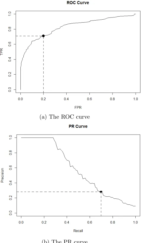
Figure 2.1 The ROC curve and PR curve for an unbalanced data. The unbalanced ex-ample dataset is composed of 100 positive and 1000 negative objects. The point (0.2,0.7) shown in ROC space corresponds to the point (0.7,0.26) on PR space. The point represents that 270 out of 1100 objects are clas-sified as positive. Among 270 clasclas-sified positives, only 70 observations are correct and 200 observations are incorrect. . . 19 Figure 2.2 Scatter plot for the contrived example data. The bivariate X data is
composed of 30 positives and 80 negatives. Red plus symbol refers to the object in the positive group; blue minus symbol indicates the object in the negative group. . . 24 Figure 2.3 ROC curves and PR curves for the scoring S1 and S2. . . 26
Figure 2.4 (a) Simulated data pattern; (b) The averaged vectors over 100 datasets for PR maximizer vs. ROC maximizer. . . 29 Figure 2.5 The averaged PR curves and ROC curves for the optimal linear PR
classi-fiers and ROC classiclassi-fiers over 100 datasets, and the averaged AUC values. The subfigures from (a) to (d) in order are: the PR curve produced by optimal PR classifiers; the PR curve produced by optimal ROC classifiers; the ROC curve produced by optimal PR classifiers; and the ROC curve produced by optimal ROC classifiers. . . 31 Figure 2.6 False discovery rate comparison between the optimal linear classifiers by
the PR curve and the ROC curve on data with different proportions of positivesπ. . . 33 Figure 2.7 False positive rate comparison between the optimal linear classifiers by
the PR curve and the ROC curve on data with different proportions of positivesπ. . . 34
Figure 3.1 The approximation of the sigmoid function, s(x) = 1
1 + exp(−x/σN) , to
the indicator function, and its first derivative with respect tox,s0(x) = exp(−x/σN)
σN(1 + exp(−x/σN))2 ,
under different values of the scale parameterσN. . . 43 Figure 3.2 The comparisons between AUCFW and LogFW algorithms on the
pre-dicted AUCROC value over the test sets. Two graphs are generated for each real data: one plots ”the predicted AUCROC vs. the number of se-lected variables” and the other plots ”the predicted AUCROC vs. p-value”. 69 Figure 3.3 Solution path presented in the ROC curves for Data #1, whereN = 500,
Figure 3.4 Solution path presented in the ROC curves for Data #2, whereN = 500,
p= 50, π= 0.5, andβ = (0.4,0.4,0.8,0.8,0.8,0, . . . ,0)T. . . 71 Figure 3.5 Solution path presented in the ROC curves for Data #3, whereN = 500,
p= 50, π= 0.1, andβ = (0.8,0.8,0.8,0.8,0.8,0, . . . ,0)T. . . 72 Figure 3.6 Solution path presented in the ROC curves for Data #4, whereN = 500,
p= 50, π= 0.1, andβ = (0.4,0.4,0.8,0.8,0.8,0, . . . ,0)T. . . 73 Figure 3.7 Solution path grid on p-value presented in the partial ROC curves and
the PR curves for Data #1A, where N = 500, p = 50, π = 0.5, and
β = (0.8,0.8,0.8,0.8,0.8,0, . . . ,0)T. . . 74 Figure 3.8 Solution path grid on p-value presented in the partial ROC curves and
the PR curves for Data #1B, where N = 500, p = 50, π = 0.5, and
β = (0.4,0.4,0.8,0.8,0.8,0, . . . ,0)T. . . 75 Figure 3.9 Solution path grid on p-value presented in the partial ROC curves and
the PR curves for Data #1As, where N = 500, p = 50, π = 0.1, and
β = (0.8,0.8,0.8,0.8,0.8,0, . . . ,0)T. . . 76 Figure 3.10 Solution path grid on p-value presented in the partial ROC curves and
the PR curves for Data #1Bs, where N = 500, p = 50, π = 0.1, and
β = (0.4,0.4,0.8,0.8,0.8,0, . . . ,0)T. . . 77 Figure 3.11 Investigation in prediction: predicted AUCROC vs. the number of variable
selected for Data #1, wherep= 50,π= 0.5, andβ= (0.8,0.8,0.8,0.8,0.8,0, . . . ,0)T. 78 Figure 3.12 Investigation in prediction: predicted AUCROC vs. the number of variable
selected for Data #2, wherep= 50,π= 0.5, andβ= (0.4,0.4,0.8,0.8,0.8,0, . . . ,0)T. 79 Figure 3.13 Investigation in prediction: predicted AUCROC vs. the number of variable
selected for Data #3, wherep= 50,π= 0.1, andβ= (0.8,0.8,0.8,0.8,0.8,0, . . . ,0)T. 80
Figure 3.14 Investigation in prediction: predicted AUCROC vs. the number of variable
Chapter 1
Introduction
1.1
Binary Classification Problems
Binary classification is one of the most widely discussed topics, which have received a great
amount of attention in various research areas, including medical diagnosis, credit scoring, and
anomaly detection. Classification is to construct a rule that maps each object to a predicted
class based on a set of training objects whose memberships are known. Consider a binary
classification problem with outcome Y ∈ {0,1}, whereY = 1 denotes the positive group and
Y = 0 is the negative group. For each object, ap-dimensional covariate vector is measured and
is denoted asX ∈Rp. Without loss of generality, assume that the classification rule is given by:
ˆ
Y =I(g(X)≥c), (1.1)
for some function g(·) and threshold c, where I is the indicator function. The score, g(X),
generates an ordering among objects, while the thresholdccreates a classification decision from
this ordering. Thus, in general, there are two types of classifiers. One is a discrete classifier that
gives a hard-labeled outcome. The other is called a scoring classifier that generates an ordered
object ranking by score values. The object ranking indicates that the one with higher score value
interested in the ranking score rather than the hard-labeled outcome, since a ranking not only
provides the potential label assignment but also conveys information about the ordering among
objects. If the function g(X) takes a linear combination of covariates X, βTX, it indicates a
linear classifier. Furthermore, suppose there are N objects involved, among which n subjects
are from the positive group and the remainingm =N −n ones belong to the negative group.
The proportion of positives among the whole population is introduced to describe the class
label distribution, which is defined as π = Pr(Y = 1) in population and can be estimated as
ˆ
π =n/N under a random sampling. The data is balanced when the number of objects in each
group is approximately equal, e.g.π = 0.5; on the other hand, the data is unbalanced when the
majority of the objects belong to one group, e.g. π = 0.1 or 0.9.
Table 1.1: Confusion Matrix
Actual Class
p n
P True False
Predicted Positives Positives Class
N False True
Negatives Negatives
Given an object and a threshold c in the classification rule (3.1), there are four possible
classification outcomes:
• True positive: a correctly classified positive object;
• False positive: a misclassified negative object;
• True negative: a correctly labeled negative object;
• False negative: a incorrectly classified negative object.
by a confusion matrix as in Table 1.1. It is a 2 by 2 table, and each cell counts the number of
objects having the corresponding outcome. As the thresholdcin the classification rule is varied,
a series of confusion matrices are generated.
Both the Receiver Operating Characteristic (ROC) curve and the Precision-Recall (PR)
curve are widely used techniques to visualize a series of confusion matrices and evaluate the
classification performance of a scoring classifier. Since the superiority of a classifier can be
determined by the ROC or PR curve, we intend to implement these two curves to construct
classifiers. Here are the introductions about the ROC curve and the PR curve.
1.2
Receiver Operating Characteristics Curve
The ROC curve was first developed for assessing the accuracy of radar equipments in battlefields
during World War II, and was soon introduced to psychology for perceptual detection of stimuli
study (Egan (1975), Swets (1973)). Swets and Pickett (1982) brought the theory and the practice
of the ROC curve to the biomedical realm, and then the ROC technique was widely treated as a
comprehensive guide to make medical decision. Over the years, the ROC curve also increasingly
gained attention for model evaluation and classifier selection in many applications of machine
learning (Bradley (1997), Spackman, Kent A. (1989)). In summary, the ROC curve is useful to:
(1) evaluate the discriminatory ability of a ranking score to correctly assign class labels; (2) find
an optimal cut-off point to best classify the two-group objects; (3) compare the classification
performances among two or more classifiers; and (4) select variables to construct a optimal
classifier that maximizes diagnosis accuracy.
The ROC curve represents the tradeoff between false positive rate (FPR = 1- specificity)
vs. true positive rate (TPR = sensitivity). Since the metrics in ROC space are defined based on
the confusion matrix, both of them are functions of the threshold c and given as FPR(c) and
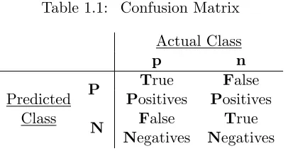
Figure 1.1: ROC Space
Then the metrics are written by:
FPR = FP
FP + TN, TPR =
TP
TP + FN. (1.2)
Since the denominators for the ROC metrics in (3.4) are fixed, the value for either FPR or TPR
increases as the threshold c gets larger. Thus, TPR is a monotonically increasing function of
FPR.
In ROC space in Figure 1.1, three important points need to be introduced. The origin point
A (0, 0) is the curve starting point, which represents the strategy of never assigning an object
to the positive group. On the other hand, the upper right corner point C (1, 1) is the curve
endpoint and represents the strategy of unconditionally predicting objects as positives. If the
curve reaches the point B (0,1), then it indicates a perfect separation, where all positives are
positioned ahead of negatives. Besides, the diagonal line in ROC space represents the strategy
upper left triangle leads to a better classification outcome than a random guess does.
In addition to TPR and FPR, the area under the ROC curve (AUCROC) is also one of
the metrics that summarize the whole curve as well as the discriminatory accuracy of a scoring
classifier. The AUCROC is defined by:
AUCROC =
Z 1
0
TPR dFPR. (1.3)
This integral area is a portion of a unit square, so its value is always between 0 and 1. Without
any assumptions on the data, one intuitive empirical approach to estimate the integral area in
Equation (3.2) is interpolating points using a step function with jumps at the data values. The
rationale is that any value between two adjacent data values doesn’t change the label
assign-ments. Given a decreasing ranking, by treating the score value of each object as a threshold,
we obtainN rectangles in ROC space and the estimation of AUCROC is denoted as
ˆ
AUCROCRec=
N
X
i=1
(FPRi−FPRi−1)×TPRi, (1.4)
where FPRi and TPRi are the corresponding rate values when theith object in the decreasing ranking is treated as the threshold in the classification rule (3.1), and FPR0= 0. This rectangle
estimation AUCROCˆ Rec is also equivalent to the one by adopting the empirical cumulative
density functions for positive and negative groups respectively. Besides, Bamber (1975) gave
an important statistical property to AUCROC by linking the integral area with a probability
expression as:
AUCROC = Pr(g( ˜X1)> g( ˜X0)), (1.5)
where ˜X1 denotes a randomly picked positive object and ˜X0 is a randomly picked negative
object. Replacing the probability in (1.5) by its empirical version, we obtain the estimated
and McNeil (1982) ), which is expressed as:
ˆ
AUCROCMW=
1 nm n X i=1 m X j=1
I(g(X1i)−g(X0j)>0), (1.6)
where X1i is the covariate vector for the ith object in the positive group, and X0j is the covariate vector for the jth object in the negative group. Although the empirical estimated
ˆ
AUCROCMW in Equation (2.11) has nice interpretation and is easy to compute, it is not a
continuous or differentiable function. Thus, it becomes a challenging task to obtain the optimizer
using AUCROCˆ MW as the target function. In order to make AUCROCˆ MW differentiable, the
sigmoid function, s(x) = 1/(1 + exp(−x/σN)), is adopted to smooth the indicator function in
Equation (2.11), and then the approximated AUCROC is given by:
ˆ
AUCROCMWS=
1 nm n X i=1 m X j=1 1
1 + exp − g(X1i)−g(X0j)
/σN
, (1.7)
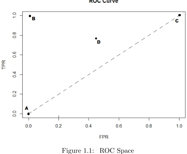
whereσN is a scale parameter. The scale parameterσN determines the magnitude of the sigmoid
function’s approximation to the indicator function. Figure 3.1 shows the plots of the sigmoid
function under different values of σN. The plot in Figure 3.1(a) displays a somewhat linear
fashion under σN = 2, thus it is a poor approximation to the indicator function. On the other
hand, Figure 3.1(b) gives a perfect approximation underσN = 0.05. Therefore, in order to make
the sigmoid function approximate the indicator function excellently, we need to obtain a small
σN value, which leads to large value of|x/σN |.
Recall that the empirical AUCROC estimations in Equations (1.4), (2.11) and (1.7) only
depend on the ranking score produced by the functiong(X). There are two remarks about the
functionality of the scoring classifiers. First, any constant adding to the score value does not
alter the object ranking or the empirical AUCROC estimations. So it is fair to assume that no
intercept is included in the scoring classifier g(X). Second, any multiplier to the current score
value does not alter the object ranking either. In other words, g(X) is only identified up to a
(a)σN = 2 (b)σN = 0.05
Figure 1.2: The approximation of the sigmoid function, s(x) = 1/(1 + exp(−x/σN)), to the indicator function for different values of the scale parameter σN.
anchor and its coefficient estimate should be fixed with norm of 1.
In literature, in addition to the aforementioned empirical AUCROC estimations, there are
also other non-parametric estimation methods proposed for AUCROC estimation, e.g. Faraggi
and Reiser (2002) obtained a non-parametric estimation of AUCROC by adopting Gaussian
kernels to estimate probability density functions for positive and negative groups respectively.
Besides, the underlying binormal distribution is the most commonly considered assumption
for parametric AUCROC estimation, where the covariate vectors for both positive and
neg-ative follow normal distributions. Hanley (1998) discussed the robustness of binormal latent
distribution for ROC curve fit; Gu and Ghosal (2009) obtained AUCROC under binormal
as-sumption by Bayesian approach using a rank likelihood; and Gon¸calves et al. (2014) gave a
broad overview on the Bayesian approach to estimate AUCROC both semi-parametrically and
non-parametrically.
For a long time, AUCROC has been used as a standard tool to evaluate diagnosis
accu-racy and compare classification performance among algorithms. Nowadays, many researches
(2003) adopted the ROC curve to rank diagnostic performance of genes in microarray
experi-ments; Ma and Huang (2005) implemented the threshold gradient decent algorithm to obtain
the coefficients for selected biomarkers by maximizing AUC and then applied cross-validation
approach to determine the optimal classifier; and Graf and Bauer (2009) investigated the
rela-tionship between false discovery rate threshold for multiple tests control and the optimal AUC
value for future independent population prediction so as to determine the number of variables
to be chosen.
1.3
Precision-Recall Curve
Figure 1.3: PR space
The PR curve is considered as a desirable alternative to the ROC curve when the class
label distribution is highly unbalanced. It was originally introduced to evaluate information
where the non-relevant queries are the majority (Raghavan et al. (1989a)). Recently, it gained
great attention in the machine learning as well (Peltonen and Kaski (2011)). The PR curve
describes the tradeoff between recall and precision as the threshold c in the classification rule
(3.1) is varied. As functions of the thresholdc, the two rate metrics in PR space are defined as:
Recall = TP TP + FN, Precision = TP
TP + FP = 1−FDR.
(1.8)
Since the denominator of precision changes as c varies, there is no certain patten displayed between recall and precision.
In PR space, the three important points shown in Figure 1.3 have the same interpretation
as those in ROC space, however they have totally different locations. The PR curve starts from
the upper left corner A (0,1), where no objects are misclassified, and ends at the point C (1,π).
The endpoint of the PR curve is not a fixed point as the one in ROC space. It depends on one
data’s proportion of positives. More skewed the data is, lower the curve endpoint is located.
Besides, the upper right corner B (1,1) is the point that represents the perfect separation.
Furthermore, one important measure to evaluate the classification performance in PR space,
which is the area under the PR curve (AUCPR), is given by:
AUCPR =
Z 1 0
Precision dRecall. (1.9)
Similar to AUCROC, this integral area is also ranged from 0 to 1. Besides, the empirical
estimated AUCPRˆ Rec can be obtained by using a step function to interpolate points in PR
space. Given a decreasing ranking, it is written as:
ˆ
AUCPRRec=
N
X
i=1
(Recalli−Recalli−1)×Precisioni, (1.10)
(AP) estimation. It is known that the value of recall alters only when a true positive object is
classified correctly and the difference between any two adjacent recall values is identical. So we
can calculate AUCPRˆ Rec using the precision value when one positive object is treated as the
threshold. Thus, AUCPRˆ Recin Equation (1.10) can be simplified as
ˆ
AUCPRRec=
1
n
n
X
j=1
Precision(X1j), (1.11)
where Precision(X1j) is the precision value when thejth positive object is classified as positive among a decreasing object ranking. In addition to AUCPRˆ Rec estimator, Boyd et al. (2013)
discussed other AUCPR estimators as well, such as trapezoidal estimator, interpolation
esti-mator, etc. Similar to AUCROC, the underlying binormal distribution is also a widely used
assumption to calculate AUCPR (Brodersen et al. (2010)). Besides, Keilwagen et al. (2014b)
derived and discussed AUCPR for binary classification with soft labels.
1.4
Relationship between the ROC Curve and the PR Curve
The metrics in both PR space and ROC space are defined based on the confusion matrices, so
these two curves share many common features. Davis and Goadrich (2006) showed that for any
dataset with fixed numbers of positive and negative objects, points can be one-to-one translated
between the ROC and PR spaces. However, the two curves also have a lot of differences. The
classifier that maximizes AUCROC doesn’t always optimize AUCPR, and vice versa (Davis and
Goadrich (2006)).
Comparing the metrics’ definitions, we notice that recall is the same as TPR. The difference
between the metrics of ROC and PR is the denominator of FPR versus that of FDR. We see
that FPR considers the total number of true negative objects; while FDR instead takes the
number of predicted positive objects into consideration. This difference is analogous to the
difference between Type I error and FDR in that the ROC curve relates to Type I error, while
sensitivity towards the skewness of class label distribution of the two curves. The ROC curve
is insensitive to the class label distribution, while the PR curve is extremely sensitive. For
the ROC curve, either TPR or FPR focuses only on the portion of objects that are labeled
correctly within each group. Thus, in the situation where the negative objects are the majority,
the ROC curve would not be able to detect the large number of incorrectly labeled negatives,
because such great number results in only a small portion compared to the totally number
of negative objects. For the PR curve, on the other hand, precision is able to capture and
reflect such situation. Knowing the positive is the minority, the slightly changed numerator
over the dramatically increased denominator would definitely alert that too many negatives are
misclassified.
1.5
Two sample U-Statistics
The empirical estimated AUCROC in Equation (1.7) is a two-sample U-statistics. So does its
first derivative with respect to the coefficient, if g(X) takes a linear functionality as βTX. In
the third chapter, we took advantage of the property of the two-sample U-statistics to conduct
forward selection, when treatingAUCROCˆ MWS as the target function. Thus, we give a general
and brief introduction about U-statistics in this chapter.
U-statistics, a distribution-free unbiased estimator, was first introduced by Hoeffding (1948),
and had asymptotic normal distribution in large samples. Hoeffding (1961) developed H-decomposition
to further discuss its asymptotical property. In addition to Wassily Hoeffding’s theoretical
con-tribution to U-statistics, Sproule (1974) developed a Kolmogorov-like inequality to examine the
converge properties; Ahmad (1981) discussed the rates of convergence in central limit theory;
and Lenth (1983) investigated interesting characteristics of U-statistics by linking the
jack-knife procedure with the existed properties. Meanwhile, U-statistics has great impact and wide
applications on non-parametric inference. Fu (2012) applied one-sample U-statistics to assess
the asymptotic distribution of a non-parametric estimator for the multivariate functional data
asymp-totic results for some inequality and poverty measures. Moreover, for two-sample U-statistics,
Dehling and Fried (2012) derived the asymptotical distribution of the two-sample empirical
U-quantiles in the case of correlated data; Dehling et al. (2013) studied a robust test for detecting
change-points of a stochastic process based on the two-sample Wilcoxion test statistics. For
problem of the variable selection, Song and Ma (2010) implemented U-statistics in penalized
variable selection using LASSO and ridge.
Suppose we have ˜X11, . . . ,X˜1n, ˜X01, . . . ,X˜0m independently and identically distributed (i.i.d.) with cumulative distribution functions F1 and F0, then a kernel ψ is a function defined
withk+l arguments
ψ(X11, . . . , X1k;X01, . . . . , X0l)
which is symmetric in each set of arguments. Then the corresponding two-sample U-statistics
based onψ has the form
Un,m=
n k −1 m l −1 X
(n,k)
X
(m,l)
ψ(X11, . . . , X1k;X01, . . . , X0l), (1.12)
where (n, k) represents all possible unordered subsets ofkelements chosen without replacement
from the set{X11, X12, . . . , X1n}, and the same interpretation for (m, l) in the set{X01, X02, . . . , X0m}. Moreover, it can be shown thatUn,m is an unbiased estimator for
θ=R ···R
ψ(u1, . . . , uk;v1, . . . , vl) k
Q
i=1
dF1(ui) l
Q
j=1
dF0(vj).
Based on Hoeffding (1961)’s decomposition, U-statistics can be decomposed into a sum of
uncorrelated components. We take two-sample U-statistics withk=l= 1 as an example, and
write it in general as
ψ(X1i, X0j) =θ+h1,0(X1i) +h0,1(X0j) +g(X1i, X0j), (1.13)
h1,0(X1i) =ψ1,0(X1i)−θ
h0,1(X0j) =ψ0,1(X0j)−θ
g(X1i, X0j) =ψ(X1i, X0j)−h1,0(X1i)−h0,1(X0j)−θ.
Since both ˜X1i and X˜0j are independent random variables with the same distribution respec-tively, it is obvious to find that h1,0( ˜X1i) and h0,1( ˜X0j) are also independently distributed with
E(h1,0( ˜X1i)) = 0, V ar(h1,0( ˜X1i)) =ς12,0;
E(h0,1( ˜X0j)) = 0, V ar(h0,1( ˜X0j)) =ς02,1.
Therefore, the two-sample U-statistics in (1.12) withk=l= 1 can be written as
U =θ+H1,0+H0,1+R, (1.14)
whereH1,0=n−1Pin=1h1,0( ˜X1i), H0,1 =m−1Pmj=1h1,0( ˜X0j), andR is the remaining element whose variance has a lower order infinitesimal of sample size. Thus, it is easy to proof that,
by large number theory,n12H1,0 and m 1
2H0,1 both converge to normal distributions with mean
zero and variances ς12,0 and ς02,1 respectively. Moreover, let N =n+m and n/N → p1 ∈ (0,1)
asnand m→ ∞, then we have
√
N(U−θ) =√N H1,0+H0,1+R
= r N n √ n n P i=1
h(1,0)(X1i)
n + r N m √ m m P j=1
h(0,1)(X0j)
m +op(1).
Since H1,0 and H0,1 are independent, it follows thatN
1
2(U −θ) converges in distribution to a
normal random variable with zero mean and variance p−11ς12,0 + (1−p1)−1ς02,1. Therefore, the
asymptotic distribution for a single two-sample U-statistics in (1.14) is written by
√
N(U(q)−θ(q))−→D N(0, p−11ς1(q,0)2+ (1−p1)−1ς0(q,1)2). (1.15)
gener-alized to the case of a U-statistics vector U = (U1, . . . , U(p))T, where the components in the vectorUare defined based on the same two independent sampleX11, . . . , X1nandX01, . . . , X0m. Then the joint limiting distribution ofUis a multivariate normal distribution. IfF1 andF0 are
continuous and both of their second moments exist, then asn→ ∞ and m→ ∞, by applying
the central limit theorem, the joint distribution of
√
N(U(1)−θ(1)),√N(U(2)−θ(2)), . . . ,√N(U(p)−θ(p))
converges to a multivariate normal distribution with zero vector mean and the limiting
variance-covariance matrix Σlim. Furthermore, the asymptotic variance-covariance matrix can be
ob-tained asΣlim= (σ
2((s),(t)
lim ), where
σ2((lims),(t)= 1
p1
ς12((,0s),(t))+ 1 1−p1
ς02((,1s),(t)),
withn/N →p1 ∈(0,1).
1.6
Dissertation Outline
In this dissertation, we investigate two patterns of datasets and develop the best approaches
to obtain the optimal linear classifier using AUC respectively. In Chapter 2, we focus on the
unbalanced data, where the majority of objects belong to the negative group. The gold standard
tool AUCROC fails to select the optimal linear classifier in terms of the object ranking due to
its insensitivity to the class label distribution. We take the advantage of PR curve’s control on
FDR, and construct the optimal linear classifier, which positions the majority of positive objects
ahead of negative ones. Since the accuracy of AUC estimation is not the primary interest, we
adopt the rectangle estimation for both AUCROC and AUCPR. The superiority of PR curve
over ROC curve on the unbalanced data is shown in simulation studies.
In Chapter 3, we developed a ROC-based variable selection algorithm to obtain the optimal
subset of variables. The algorithm treats AUCROC as the target function to be maximized,
likelihood-based hypothesis statistics, we adopt score statistics to be the selection criterion as
well as the stopping rule. In order to make AUCROC differentiable, the empirical estimated
ˆ
AUCROCMWS is used. We further show the score function derived from AUCROCˆ MWS is a
two-sample U-Statistics, and follows an asymptotic normal distribution. Simulation studies in
different scenarios, e.g. magnitude of correlation between covariates, are conducted to compare
the proposed AUCROC forward selection algorithm with the regular linear logistic regression
using forward selection by the whole solution path as well the relation between p-value and the
Chapter 2
Classification for Highly Unbalanced
Data by Maximizing the Area Under
the Precision-Recall Curve
2.1
Introduction
Binary classification problems have received a great amount of attention in various research
areas, including medical diagnosis, credit scoring, and anomaly detection. Consider a binary
classification problem with class label Y ∈ {0,1} indicating negative and positive group
as-signment, and predictor variable vector X ∈ Rp. If the number of objects in each group is
approximately equal, then we say the data is balanced; on the other hand, if the majority of the
objects belong to one group, the data is unbalanced. Without loss of generality, assume that
the classification rule is given by
ˆ
Y =I(g(X)≥c) (2.1)
for some function g(·) and a threshold c. The score, g(X), gives the rank order of the objects,
g(X) takes a linear combination of the predictor variable vectorX, which isβTX, it indicates
a linear classifier. In many instances, researchers are more interested in the ranking score rather
than the hard-labeled outcome, since a ranking not only provides the potential label assignment
but also conveys information about the ordering among objects.
For a fixed thresholdc, the performance of a classifier can be assessed by a confusion matrix as in Table 1.1. A confusion matrix is composed of four components:
• True positives (TP): the number of positive objects correctly classified as positive;
• False positives (FP): the number of negative objects incorrectly classified as positive;
• True negatives (TN): the number of correctly labeled negative objects;
• False negatives (FN): the number of misclassified positive objects.
An overall picture of a classifier can then be viewed as a series of confusion matrices as the
threshold varies.
The receiver-operating characteristic (ROC) curve is a widely used approach and often
con-sidered as a gold standard to visualize a series of confusion matrices. The plot of the ROC curve
represents the trade-off between true positive rate (TPR) and false positive rate (FPR), where
TPR measures the fraction of positive objects that are correctly labeled and FPR measures
the fraction of negative ones that are misclassified as positive. The area under the ROC curve
(AUCROC), given in (3.2), is the most common scalar measurement that summarizes the curve,
as well as the performance of a score ranking.
AUCROC =
Z 1
0
TPR dFPR (2.2)
Larger AUCROC leads to a better overall classification performance. For a long time, the
AUCROC is widely used to evaluate classification performance. Recently many researchers
AUCROC as the objective function for combining biomarkers for classification; Ma and Huang
(2005) implemented an AUCROC-based Threshold Gradient Descent Regularization algorithm
to select important biomarkers for disease classification; Marrocco et al. (2008) constructed
a nonparametric linear classifier that relied on the Wilcoxon–Mann–Whitney statistic; Castro
and Braga (2008) proposed an algorithm to maximize AUCROC based on gradient descent;
and Graf and Bauer (2009) selected a best classification model that optimizes AUCROC based
on FDR-thresholding. However, despite its popularity, the ROC curve has some drawbacks that
make it a less ideal tool to evaluate and construct classifiers under unbalanced data.
A disadvantage of the ROC curve is its ignorance to the proportion of the positive objects
relative to the negative objects. In the situation where negative objects are the majority, we
can observe two facts from ROC space, (1) a small change in FPR value indicates a large
increase in the actual number of misclassified negative objects; (2) the majority of the AUCROC
corresponds to the region of high FPR. Therefore, under unbalanced situations, false discovery
rate (FDR) can be very high in the region that dominates the curve.
As an example to demonstrate this phenomenon, consider a dataset composed of 100 positive
and 1000 negative objects. Figure 2.1(a) is an example of a ROC curve for a classification
algorithm for this unbalanced dataset. The point (0.2,0.7) shown in Figure 2.1(a) represents that
270 out of 1100 objects are classified as positive. However, among the 270 classified positives,
only 70 objects are correctly predicted and the remaining 200 are not. At the point (0.2,0.7),
where FPR is still relatively low, i.e. 0.2, the FDR reaches 200
270, which means nearly three-fourths of the classified positives are incorrect. Furthermore, we can see that the FDR would
increase as FPR gets larger, in the region where the slope of the ROC curve becomes flat.
We can see that the majority of the AUCROC is added in the region which is not of interest.
Therefore, under unbalanced cases, the ignorance to class label distribution makes AUCROC
a poor measure of classification performance, and the linear classifier obtained by maximizing
AUCROC becomes a less desirable one.
(a) The ROC curve
(b) The PR curve
the partial area under the ROC curve (pAUCROC) in (2.3) has been proposed. The partial
area is considered over a pre-specified range of FPR rather than the whole range.
pAUCROC(s) =
Z s
0
TPR dFPR, for some 0< s <1 (2.3)
For the example in Figure 2.1(a), we can constrain the range of FPR to be (0,0.2) and obtain the
optimal classifier by maximizing pAUCROC in order to meet low FDR demand. McClish (1989)
introduced pAUCROC under the binormal assumption to solve the problem when the entire
range is not of interest and proposed a test statistics to compare two partial areas; Yousef,
Waleed A. (2013) assessed the performance of a classifier by pAUCROC, and discussed its
nonparametric estimator; Ma et al. (2013) discussed pAUCROC and standardized pAUCROC
to evaluate diagnostic performance. In the context of obtaining optimal classifiers, Wang and
Chang (2011), Hsu and Hsueh (2013b) and Ricamato and Tortorella (2011) proposed algorithms
to select the best linear classifier by maximizing pAUCROC when low FPR is prerequisite; and
Komori and Eguchi (2010) developed a new pAUCROC-focused method based on a boosting
technique to construct nonlinear classifiers. However, in general, the cutoff, s, is an arbitrary
choice, and thus pAUCROC has not gained in popularity.
The precision recall (PR) curve, has become an increasingly competitive and useful
alterna-tive to the ROC curve. It plots the recall, equivalent to TPR, against the precision, or posialterna-tive
predictive rate. The area under the PR curve (AUCPR), in (2.4), is also considered as a
com-prehensive performance measure and has attracted many recent investigations (e.g. Oliphant
et al. (2010b)).
AUCPR =
Z 1
0
Precision dRecall (2.4)
Due to the sensitivity of precision to the class label distribution, AUCPR controls the number of
misclassified negatives, and consequently meets low FPR and FDR demands. Most importantly,
the AUCPR does not require a chosen bound on the region under consideration as does the
aforementioned algorithm for the unbalanced example data. The point (0.2,0.7) in ROC space
in Figure 2.1(a) corresponds to the point (0.7,0.26) in PR space shown in Figure 2.1(b). It
shows that the small partial area in ROC space corresponds to the majority of the area in
PR space. It further indicates that even when the whole range of recall is taken, the FDR is
relatively low in the dominated area of AUCPR. Therefore, AUCPR is an important tool for
classification problems under unbalanced data.
Davis and Goadrich (2006) showed that for any dataset with fixed numbers of positive and
negative objects, points can be one-to-one translated between the ROC and PR spaces. So the
ROC curve and the PR curve share many common features, but they also differ a great deal.
In this paper, we point out that the classifiers constructed by maximizing the two areas could
be very different; and demonstrate that under unbalanced situations, the classifier obtained by
maximizing AUCPR outperforms the one obtained by maximizing AUCROC in terms of FDR.
In section 2, we give brief introductions to the ROC curve and the PR curve, and
demon-strate their different preferences on score rankings by example. We introduce the empirical
area under the curve (AUC) estimation applied in this paper for the two curves in section 3.
In section 4, the implementation of maximizing AUC to obtain linear classifiers is described
in details. In section 5 we summarize the comparisons between the optimal linear classifiers
obtained by the two curves from a simulation study. Conclusion is summarized in section 6.
2.2
The ROC and PR Curves
Suppose there areN objects involved in the classification problem, among whichnsubjects are
from the positive group and the remainingm=N−nones belong to the negative group. The
proportion of positives in the population is given by Pr(Y = 1) and denoted asπ.
2.2.1 Metrics in Two Curves
Given a threshold c, the classification outcome can be represented in a confusion matrix as in
given confusion matrix. The ROC curve is composed of TPR versus FPR; while the PR curve
plots precision against recall. Equations (3.4) and (2.6) give the definitions for the ROC and
PR metrics:
FPR = FP
FP + TN, TPR =
TP
TP + FN = Recall; (2.5)
Precision = TP
TP + FP = 1−FDR. (2.6)
Notice that recall is the same as TPR. The difference between the metrics of ROC and PR
is the denominator of FPR versus that of FDR. We see that FPR considers the total number
of true negative objects; while FDR instead takes the number of correctly predicted positive
objects into consideration. This difference is analogous to the difference between Type I error
and FDR in that the ROC curve relates to Type I error, while the PR curve measures FDR.
In either ROC or PR space, one classification decision determined by a given threshold is
displayed as a single point. A ROC curve or a PR curve is obtained as the threshold varies.
Then AUC is a common metric that measures the overall classification performance.
2.2.2 Receiver Operating Characteristic Curve
The ROC curve was first developed in the early 1950’s as a signal detection technique (Swets
(1986)). One of its first application was to assess the accuracy of radar equipment in World War
II. Later the ROC curve gained attention in radiology imaging diagnosis (Lusted (1960), Metz
(1986)), as well as solving medical decision problems (Metz (1978), Lusted (1978)). Recently
it has been widely used for model evaluation and selection in many applications of machine
learning (Spackman, Kent A. (1989), Bradley (1997)). Its wide applications not only owing
to its comprehensive presentation of tradeoff between FPR and TPR, but also a summarized
number measuring classification performance, which is AUCROC. In addition to the defined
property by linking the integral area with a probability expression as:
AUCROC =P(g(Xpos)> g(Xneg)), (2.7)
whereXposdenotes a randomly picked object from the positive group and Xneg is a randomly
picked negative object. The estimation for AUCROC has been widely discussed in both
para-metric and non-parapara-metric approaches. For parapara-metric approaches, based on the underlying
binormal distribution assumption, AUCROC can be represented using the standard normal
distribution. Hanley (1988) discussed the robustness of binormal latent distribution for ROC
curve fit; Tosteson and Begg (1988) applied ordinal regression model to estimate the ROC curve
parameters and its AUC for categorical rating data; Gu and Ghosal (2009) obtained AUCROC
under the binormal assumption via a Bayesian approach. For AUCROC estimation, replacing
the probability in (2.7) by its empirical version, we obtain the AUCROC value as equivalent to
the Mann-WhitneyU-statistics (Hanley and McNeil (1982)), given by
ˆ
AUCROC(β) = 1
nm
n
X
i=1
m
X
j=1
I(g(Xpos,i)−g(Xneg,j)>0), (2.8)
whereXpos,i indicates theith object in the positive group andXneg,j refers to thejth object in the negative group.
2.2.3 Precision Recall Curve
As an alternative to the ROC curve, the PR curve was originally introduced to evaluate
in-formation retrieval system by judging both efficiency and effectiveness of the whole retrieval
process (Raghavan et al. (1989b)), and have been gaining popularity for classification
per-formance evaluation under unbalanced data. AUCPR, as a counterpart of AUCROC, can be
interpreted as average precision. Similar to AUCROC, an underlying binormal distribution is
one widely used parametric assumption to calculate AUCPR (Brodersen et al. (2010)). For
that linear interpolation is not appropriate in PR space when two points are far apart due to
its varied denominator of precision, and then proposed an expression for the intermediate PR
point. Cl´emen¸con and Vayatis (2009) introduced a nonparametric approach to assess PR curve,
and examined its related theoretical and practical issues; Boyd et al. (2013) discussed several
different approaches to compute empirical AUCPR point estimators, e.g. trapezoidal estimator,
interpolation estimators, and obtained confidence intervals by performing bootstrap procedure;
Keilwagen et al. (2014a) pointed out AUCPR is highly informative about the classifier
perfor-mance, and discussed AUCPR for weighted and un-weighted data.
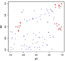
2.2.4 A Simple Example
To further investigate the different behaviors for score rankings under the ROC curve and
the PR curve, we will give a simple contrived example. Consider a bivariate X, where the data is
composed of 30 positives and 80 negatives. Figure 2.2 displays the scatter plot for this example
data. We investigate two candidate linear classifiers. The first linear classifier is the classifier
according to the variablex1, while the second one would be according tox2. These two classifiers
generate the rankingS1 and S2 correspondingly.
S1 :
20 times
z}|{
1...1
70 times
z}|{
0...0
10 times
z}|{
1...1
10 times
z}|{
0...0
S2 :
10 times
z}|{
1...1
30 times
z}|{
0...0
20 times
z}|{
1...1
50 times
z}|{
0...0
Comparing the two rankings above, we see that, S1 places 20 positive objects at the top
of the ordering, so we are able to have 20 correctly classified positives without any mistakes.
Meanwhile we would need to consider sacrificing the remaining 10 positives positioned at the
tail, in favor of zero-misclassified 20 positives. In rankingS2, there are only 10 positive objects
listed at the top. Thus, if more than 10 positive objects are desired, we will be required to include
30 misclassified negative objects. Therefore, under the situation where the positive group is the
minority, S1 is still able to keep most of the positives at the top of a score ranking, while S2
would result in many false positive objects if we want to keep a significant number of positive
label correctly.
Observing the corresponding ROC and PR curves and AUC values for the ranking S1 and
S2 in Figure 2.3, we are able to tell the different preferences these two curves have. In ROC
space, the top 20 positive objects in the rankingS1lead to relative higher TPR than the ranking
S2 does when FPR is low. However, when we look at FPR above 0.4, thenS2 has a large jump.
This region that is not likely of interest adds the most area. Because of this, the ROC curve
prefersS2 with an area of 0.75 over S1 with an area of 0.71. On the other hand, the PR curve
shows the opposite selection. The PR curve generated by the ranking S1 stays at value 1 of
precision longer than the one byS2, so the overall AUCPR of S1 is higher with area value 0.76.
(a) the ROC curve forS1
with AUCROC = 0.71
(b) the ROC curve forS2
with AUCROC = 0.75
(c) the PR curve forS1
with AUCPR = 0.76
(d) the PR curve forS2
with AUCPR = 0.6
thex2 direction, while the PR curve prefers the one towards thex1 direction. Moreover, we can
conclude that, in general, the linear classifier that positions more positive objects at the top
would outperform in PR space. This seems like a more desirable outcome in typical cases.
2.3
AUC Calculation
The primary interest in this paper is to construct an optimal linear classifier by maximizing
AUC, which takes the form ofβTXin the classification rule (3.1). Thus, in this section, we
com-pute the metrics for both two curves based on linear classifiers, and specify the corresponding
AUC calculations.
Recall that either AUCROC or AUCPR is determined by a score ranking among objects.
Since our focus is on constructing the optimal classifiers by maximizing the AUC rather than
the accuracy of the AUC values, the method of interpolation that we use does not effect our
results. Therefore, we implement the intuitive empirical approach resulting in a step function
with jumps at the data values. By treating the score value of each object as a threshold in
the classification rule (3.1), we are able to obtain n possible classification outcomes based on
the data, which consequently generate n rectangles in either of the two spaces. Then given
the ordered ranking, we can estimate AUCROC and AUCPR as the summation ofnrectangle
areas, and written by
ˆ
AUCROC(β) = n
X
i=1
(FPR(β)i−FPR(β)i−1)×TPR(β)i, (2.9)
ˆ
AUCPR(β) = n
X
i=1
(recall(β)i−recall(β)i−1)×precision(β)i, (2.10)
where the index i denotes the ith object among the decreasing ranking, and the data-based metric rates are calculated as
• TPR(β)i = recall(β)i =
Pn
j=1I(βTXj ≥βTXi|Yj = 1)
Pn
j=1I(Yj = 1)
• FPR(β)i=
Pn
j=1I(βTX ≥βTXi|Y = 0)
Pn
j=1I(Yj = 0)
,
• precision(β)i=
Pn
j=1I(Yj = 1|βTXj ≥βTXi)
Pn
j=1I(βTXj ≥βTXi) ,
• FPR(β)0 = recall(β)0 = 0 under the assumption that the plot starts from the origin
(0,0).
As an alternative to the expression for the AUCROC in (2.9), we can also estimate AUCROC
empirically using the expression in (2.8). Given a linear classifier βTX, we have
ˆ
AUCROC(β) = 1
nm n X i=1 m X j=1
I(βTXpos,i−βTXneg,j >0). (2.11)
2.4
Optimization
In this section, we concentrate on describing the approach to obtain optimal linear classifiers
on both ROC and PR spaces, and illustrating the optimization implementation in details.
Either of the AUCROC estimation in (2.9) or the AUCPR estimation in (2.10) is a function
of β, so the target function is to find the optimal β that maximizes AUC and can be written,
in general, as
ˆ
β = argmax{AUC(β)}. (2.12)
First note that the objective function, which results from either (2.10) or (2.11), only depends on
the ranking of βTXi, and changing β will not change the ranking on a small region. Therefore,
the target function (2.12) is a non-linear and non-differentiable function with respect toβ. To
optimize, we use Nelder and Mead (1965) ’simplex’ direct search method.
In addition to the non-linear and non-differentiable property of the target function, there
are two additional issues involved. First is the identifiability of β, and second is the choice of initial starting point in the optimization.
Constructing a linear classifier is to find a vector direction that produces a score ranking
Addition-ally,β is only identified up to a scalar-multiple. In order to make β identifiable, we choose one
variable as an anchor and fix its coefficient estimate to have norm of 1. The predictor variable
that has the maximal marginal AUC is selected as the anchor, and then its corresponding
esti-mate is set to be 1 or -1, depending on the direction of its marginal maximizer. The coefficient
estimation from a linear logistic regression model is applied as the starting value forβ, rescaling
so that the anchor has magnitude of 1.
2.5
Simulation Study
We now conduct a simulation to support the conclusions that (1) the linear classifier by
opti-mizing the PR curve is different from the one by optiopti-mizing the ROC curve; and (2) the optimal
PR linear classifier outperforms the optimal ROC classifier in terms of FDR.
(a) (b)
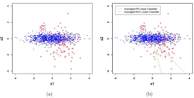
Figure 2.4: (a) Simulated data pattern; (b) The averaged vectors over 100 datasets for PR maximizer vs. ROC maximizer.
inves-tigated, wherex1 and x2 represent the covariate values for each observation. The data pattern
is composed of 1000 points with 100 positives, so π = 0.1. The data points belonging to the
positive group denoted in red (+) in Figure 2.4(a) are generated from a mixture of normal
distributions,
X|Y=1 ∼p*N
1
−0.8
, 1 0
0 1.2
+ (1-p)*N −1
1.5
,
0.2 0
0 0.2
,
where N(µ,Σ) denotes a normal distribution with mean µ and covariance matrix Σ ,and p is
the probability from the first normal distribution, which is set to be 0.85 in the simulation. The
data points in the negative group denoted in blue (−) are generated from a normal distribution
as
X|Y=0∼N
0 0 ,
1.2 0
0 0.35
.
2.5.1 Different Preference in Optimal Linear Classifier
We generate 100 datasets using the data structure described above, and construct the optimal
PR linear classifiers and ROC linear classifiers by maximizing the area under the two curves
correspondingly for each dataset. Figure 2.4(b) displays two averaged vectors over the simulated
100 datasets for the PR maximizer in green solid line and the ROC maximizer in dashed brown
line, where the two vectors point towards different directions. Figure 2.5 present the averaged
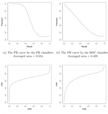
PR and ROC curves for the optimal PR and ROC classifiers correspondingly. Specifically, Figure
2.5(a) shows the averaged PR curve that is obtained via the optimal PR linear classifiers. Then
the Figures from 2.5(b) to 2.5(d) in order are: the PR curve by the optimal PR linear classifier;
the PR curve by the optimal ROC linear classifier; the ROC curve by the optimal PR linear
classifier; and he ROC curve by the optimal ROC linear classifier.
Comparing the top two figures, we see that the averaged AUCPR value at the top-left corner
(a) The PR curve by the PR classifiers Averaged area = 0.554
(b) The PR curve by the ROC classifiers Averaged area = 0.429
(c) The ROC curve by the PR classifiers Averaged area = 0.669
(d) The ROC cure by the ROC classifiers Averaged area = 0.701
that optimizes AUCROC doesn’t optimize AUCPR. The similar conclusion can be obtained for
ROC space and the optimal ROC classifier from the bottom two figures. In addition, observing
Figure 2.5(a) and 2.5(b), we find that there is a flat platform where precision stays at value
1 in PR space and a vertical line where TPR stays at value 0 in ROC space. It means the
optimal PR linear classifier intends to position positives at the early part of the ranking, and
the corresponding region likely adds the most area in PR space. However, the horizontal and
vertical flat part at the end of two curves correspondingly also indicate that the optimal PR
linear classifier meanwhile scarifies some positives by leaving at the tail of the ranking. On the
other hand, the optimal ROC linear classifier positions positive and negative objects in a more
balanced way, and try to avoid positives left behind, thus no obvious flat parts can be observed
at either the early or tail part in Figure 2.5(c) and 2.5(d).
2.5.2 Comparison of Optimal Linear Classifiers by FDR
As discussed earlier, FDR is a common criterion to measure the degree of misclassification,
particularly under the unbalanced case, and then can be used to determine the superiority of
one classifier over another. Thus, the FDR values are compared between the optimal ROC and
PR linear classifiers averaging over 100 simulated datasets. Since we are interested to examine
the impact of the data’s skewness, from a highly skewed situation to a balanced case, the
datasets with proportion of positives in{0.05, 0.1, 0.2, 0.3, 0.4, 0.5} are investigated.
Figure 2.6 displays the FDR comparisons between the optimal PR and the ROC linear
classifiers for each of the 6 positive proportions. The linear classifiers are trained on a dataset
with 1000 observations and evaluated on a testing dataset with 10000 observations. Each graph
plots the averaged FDR over 100 datasets as a function of the number of total positives correctly
identified. Thus, the range for x-axis varies for each graph depending on the total number of
positives in the dataset. In each graph, two FDR lines are generated, where the FDR line by
the ROC classifier is in red dashed line and the one by the PR classifier is the blue solid line.
(a)π= 0.05 (b)π= 0.1
(c) π= 0.2 (d)π= 0.3
(a)π= 0.05 (b)π= 0.1
(c) π= 0.2 (d)π= 0.3
ROC classifier increases in a somewhat linear fashion, while the FDR by the PR classifier stays
at zero until 25% of the positives enter. The optimal ROC linear classifiers always lead to a
higher FDR value than the optimal PR classifiers until reaching just above 50% of the true
positives. This occurs at a high FDR, somewhere between FDR of 0.3 and 0.8 depending on
the proportion of positives. Besides, more skewed the dataset is, more obvious the disparity
between two FDR lines can be observed.
In addition, the FPR comparisons between the optimal PR and ROC linear classifiers are
also examined in Figure 2.7. Each graph plots the averaged FPR against the number of true
positives correctly classified. We see that the shapes of averaged FPR curves are nearly the same
under 6 different scenarios of positive proportions. It is consistent with the fact that FPR is
ignorant to the class label distribution. Although the PR curve doesn’t focus on controlling the
metric FPR, the optimal PR linear classifiers lead to a lower FPR value than the optimal ROC
classifiers until FPR reaches 0.2. Therefore, we can reach the conclusion that, the score ranking
by the optimal PR linear classifier outperforms the optimal classifier by the optimal ROC linear
classifier in terms of FDR as well as FPR, especially under highly unbalanced situation.
2.6
Conclusion
In this paper, we provide examples to support the statement that the classifier optimizing the
ROC curve does not always optimize the PR curve, and further demonstrate that the linear
classifier obtained by the PR curve outperforms the ROC curve under unbalanced data. There
is no global rule to determine the superiority of classifiers. In general, it depends on the data
and potential misclassification costs trading off Type I vs Type II error. In the case of the
unbalanced situation, where the number of positive objects is relatively fewer comparing to
negative ones, FDR is a common measure on the number of misclassified negatives. In that
case, the number of misclassified negatives at the early part of a score ranking is minimized,
and consequently the number of correctly labeled positives is maximized. Due to the ROC
at the tail, negative objects are often positioned ahead of positives under unbalanced data,
which could lead to high FDR even early on. Although the partial ROC curve is able to meet
low FDR demand, it involves specification of threshold for FPR. On the other hand, the PR
curve is sensitive to the proportion of positive, which meets the low FDR demand and if free of
choice of threshold. Therefore, the PR curve is shown to be a worthwhile approach to construct
Chapter 3
Forward Selection via Maximizing
the Area under the ROC Curve for
Classification
3.1
Introduction
Classification and variable selection are two widely discussed topics in various research areas
and statistical applications. Consider a binary classification problem with outcome Y ∈ {0,1}
indicating the positive group and the negative group respectively, and covariate vectorX∈Rp.
Classification methods intend to construct a classification rule that maps each object to a
predicted class, e.g. positive or negative, based on a set of training objects whose memberships
are known. The classification rule, in general, takes the form as:
ˆ
Y =I{g(X)> c}, (3.1)
whereIis the indicator function,g(.) generates a score value for each object, and the threshold
the pool, while ignoring irrelevant ones. The objective of variable selection is four-fold: providing
a better understanding of the underlying relationship between outcomes, improving the accuracy
to the estimation of the interested quantities, enhancing the model’s generalization and avoiding
overfitting, and reducing time and economic cost on data collection in the future. Therefore, the
selection of variables becomes an important and essential task as hundreds to tens of thousands
of variables are currently available.
Many variable selection methods in the classification context are explored. In general, there
are three types of variable selection methods (Guyon and Elisseeff (2003)): filter, wrapper, and
embedded. The filter approach is a preprocessing step to score the importance of each variable
independently according to a particular metric, e.g. correlation coefficient, individual predictive
power, and etc. It is favored because of its simplicity, scalability, and computational efficiency.
Meanwhile, the filter method is limited because the measured score is ignorant to the other given
variables. Thus the filter method, e.g. variable ranking, is normally used as a baseline method
prior to using the variable selection metrics (Weston et al. (2003), Forman (2003)). The wrapper
approach utilizes an objective function to assess the usefulness of subsets of variables according
to their prediction performances (Kohavi and John (1997)). It is a powerful and robust tool to
find the optimal subset. Although the wrapper method is often criticized for requiring massive
of amounts of computation, forward selection and backward elimination have computational
advantages. This is because both two greedy search strategies yield nested subsets of variables.
Forward selection starts with an empty set of variables and adds one variable at each iteration
until the full set is reached; on the other hand, backward elimination begins at a full set and
removes one variable at a time. The wrapper approach is widely used and can be incorporated
with any classification algorithm, e.g. logistic regression, random forest, CART, etc. (In Lee and
Koval (1997), Peng et al. (2010), Zellner et al. (2004) ). The embedded method is an approach
that combines two terms together: the objective function to be optimized and the number
of selected variables to be minimized. Regularization method is one of the typical embedded
(Tibshirani (1996)) and forward stagewise selection to construct the optimal linear classifier;
Zhu et al. (2003) and Wang et al. (2006) introduced 1-norm and 2-norm support vector machines
in two-class classification problems respectively; and Friedman et al. (2010) developed fast
algorithms for generalized linear models with penalties of LASSO, ridge regression, and elastic.
In addition to the aforementioned methods, the receiver operating characteristic (ROC)
curve, a gold criterion to evaluate classification performance, also has wide applications dealing
with tasks for variable selection. The ROC curve assesses classification accuracy by true positive
rate (TPR) and false positive rate (FPR) of class label assignments. TPR measures the fraction
of positive objects that are correctly classified; and FPR measures the fraction of negative
objects that are misclassified as positive. The area under the curve (AUCROC) is a
threshold-free metric for performance evaluation, which is defined as:
AUCROC =
Z 1
0
TPR dFPR. (3.2)
Bamber (1975) investigated the integral area in (3.2) and gave an important statistical property
by:
AUCROC = Pr(g( ˜X11)> g( ˜X01)), (3.3)
where ˜X11 denotes a random object from the positive group and ˜X01 is a random object from
the negative group. Thus it is the probability of the score for a randomly chosen positive
object higher than the score for a random chosen negative object. Pepe et al. (2003) adopted
the ROC curve to rank diagnostic performance of genes in microarray experiments. Ma and
Huang (2005) implemented the threshold gradient decent algorithm to obtain the coefficients
for selected biomarkers by maximizing AUCROC. They then applied cross-validation approach
to determine the optimal classifier. In order to determine the number of variables to be chosen,
Graf and Bauer (2009) investigated the relationship between false discovery rate threshold
for multiple tests control and the optimal AUCROC value for future independent population