ABSTRACT
XUE, XIANGMING. Novel Robust and Adaptive Distributed Protocol for Consensus-based Control of Uncertain Multi-agent Systems. (Under the direction of Dr. Fen Wu.)
This dissertation addresses the consensus problem for linear multi-agent systems subject to uncertainty and external disturbance. A set of novel distributed robust and adaptive control protocols are designed with the knowledge of graph theory, system transformation, application of robustH∞ control and adaptive control.
A multi-agent system is a system composed of multiple interacting intelligent agents. The distributed control of multi-agent systems has great efficiency due to the team of agents operating in a coordinated fashion and reduction of computational cost. In the distributed control system, each agent has its own controller, which utilizes the local information from itself and/or its neighbors. As one of the important issues in multi-agent system control, consensus of multi-agent systems means that the states of agents reach an agreement by utilizing the local information.
In practice, it is difficult to obtain all the agent’s states due to economic reasons and constraints on measurements. Therefore, it is important to study the output feedback consensus protocol. A novel distributed dynamic output feedback controller is proposed to investigate theH∞consensus problem of linear multi-agent systems subject to external disturbance. An important contribution of this protocol lies in that theH∞output-feedback consensus synthesis conditions are, for the first time, convexified without introducing any conservatism and formulated as linear matrix inequalities, which can be solved efficiently via convex optimization.
Moreover, the agent dynamics are not all identical and precisely known. Agents usually work in different environment with uncertain dynamics and unknown external disturbance. Therefore, studying the robustness of multi-agent systems is a major issue in consensus control field. The distributed robustH∞ consensus problem for a general class of uncertain linear multi-agent systems via state and output feedback protocols were studied. The state-space matrices of the uncertain multi-agent systems depend on the structured uncertainty, which is the most general uncertainty description among the current robust consensus research field, in linear fractional transformation (LFT) form. These works are the first attempt to investigate the robust consensus with respect to a structured uncertainty of the multi-agent systems via state feedback and output feedback protocols.
Novel Robust and Adaptive Distributed Protocol for Consensus-based Control of Uncertain Multi-agent Systems
by Xiangming Xue
A dissertation submitted to the Graduate Faculty of North Carolina State University
in partial fulfillment of the requirements for the Degree of
Doctor of Philosophy
Mechanical Engineering
Raleigh, North Carolina 2019
APPROVED BY:
Dr. Aranya Chakrabortty Dr. Xiaoning Jiang
Dr. Richard F. Keltie Dr. Fen Wu
DEDICATION
BIOGRAPHY
ACKNOWLEDGEMENTS
I would like to express my sincere gratitude to my advisor Dr. Fen Wu for the continuous support of my research, for his patience, motivation, and immense knowledge throughout the last three years. His guidance helped me in all the time of research and writing of this thesis.
Besides my advisor, I would like to thank the rest of my thesis committee: Dr. Aranya Chakrabortty, Dr.Xiaoning Jiang and Dr. Richard F. Keltie for their insightful comments and encouragement, which incented me to widen my research from various perspectives.
TABLE OF CONTENTS
LIST OF TABLES . . . .viii
LIST OF FIGURES. . . ix
LIST OF SYMBOLS . . . xi
Chapter 1 INTRODUCTION . . . 1
1.1 Background . . . 1
1.2 Objectives . . . 4
1.3 Overview of related work . . . 4
1.3.1 Consensus Control . . . 4
1.3.2 Uncertainties and disturbances in multi-agent systems . . . 6
1.3.3 Communication in multi-agent systems . . . 8
1.4 Contributions . . . 9
1.5 Outlines . . . 10
Chapter 2 Preliminaries of Consensus control . . . 12
2.1 Mathematical Preliminaries . . . 12
2.2 Graph Theory . . . 16
2.2.1 Fundamental of Graphs . . . 16
2.2.2 Matrix Representation of Graphs . . . 18
2.3 Stability theory . . . 21
Chapter 3 Consensus control for Multi-agent systems with external disturbances. . . 24
3.1 Introduction . . . 24
3.2 Problem statement . . . 25
3.2.1 Model description . . . 25
3.2.2 Design Objective . . . 26
3.3 Main Results . . . 27
3.3.1 The novel output feedback consensus protocol structure . . . 27
3.3.2 Consensus under the novel protocol . . . 28
3.3.3 Stability analysis for consensus problem . . . 30
3.3.4 Performance analysis for consensus problem . . . 32
3.3.5 Convexified synthesis conditions . . . 33
3.3.6 Consensus value . . . 37
3.4 Extensions to unbalanced directed graphs . . . 38
3.4.1 DirectedH∞consensus description . . . 39
3.4.2 Consensus under the output-feedback protocol with directed graph . . . 40
3.5 LMI regions for multi-agent systems . . . 45
3.5.1 Definition of LMI regions . . . 45
3.5.2 Interesting LMI region examples . . . 47
3.5.3 H∞consensus synthesis with pole placement . . . 49
3.6.1 Definition of Laplacian spectral constraint . . . 51
3.6.2 Upper and lower eigenvalue constraints . . . 51
3.6.3 Application of graph design problems . . . 52
3.7 Simulations . . . 53
3.7.1 Compare with conventional output feedback protocol . . . 54
3.7.2 H∞consensus with LMI regions . . . 56
3.7.3 Consensus value simulation . . . 59
3.7.4 DirectedH∞consensus . . . 60
3.7.5 Laplacian spectral constraints design . . . 64
3.7.6 H∞consensus under external disturbance . . . 69
3.8 Conclusions . . . 74
Chapter 4 Robust Consensus control for Multi-agent systems with external disturbances and structured uncertainties . . . 76
4.1 Introduction . . . 76
4.2 Problem Statement . . . 78
4.2.1 Model description . . . 78
4.2.2 Objective . . . 79
4.3 Robust consensus control for multi-agent systems with structured uncertainties: State-feedback protocol . . . 80
4.3.1 The state-feedback consensus protocol structure . . . 80
4.3.2 Consensus under the state-feedback protocol . . . 80
4.3.3 Stability analysis for state-feedback consensus problem . . . 82
4.3.4 Performance analysis for consensus problem . . . 85
4.3.5 Synthesis Condition for RobustH∞Consensus . . . 88
4.4 Robust Consensus control for Multi-agent systems with structured uncertainties: Output-feedback protocol . . . 90
4.4.1 The novel output-feedback consensus protocol structure . . . 90
4.4.2 Stability analysis for output-feedback consensus problem . . . 93
4.4.3 Performance analysis for consensus problem . . . 97
4.4.4 Synthesis Condition for RobustH∞Consensus . . . 99
4.4.5 BMI Iteration Algorithm . . . 103
4.5 Robust Consensus control for Multi-agent systems with structured uncertainties: Unbalanced Directed graph . . . 104
4.5.1 Directed RobustH∞consensus description . . . 104
4.5.2 Consensus under the output-feedback protocol with directed graph . . . 105
4.6 Simulations . . . 109
4.6.1 Structured uncertain multiple Mass-Spring-Damper model description . . . . 110
4.6.2 Simulation 1: State feedback robust consensus protocol . . . 113
4.6.3 Simulation 2: output feedback robust consensus protocol with undirected network . . . 116
4.6.4 Simulation 3: Output feedback robust consensus protocol with large-scale agents . . . 119
Chapter 5 Novel Distributed Output-Feedback Adaptive Consensus Protocol for
Multi-Agent Systems. . . .130
5.1 Introduction . . . 130
5.2 Problem Statement . . . 131
5.2.1 Model description . . . 131
5.2.2 Objective . . . 132
5.3 Main Results . . . 132
5.3.1 The novel adaptive protocol structure . . . 132
5.3.2 Consensus under the novel adaptive protocols . . . 133
5.3.3 Stability analysis for adaptive consensus problem . . . 134
5.3.4 Performance analysis for adaptive consensus problem . . . 138
5.3.5 Convexified synthesis conditions . . . 141
5.3.6 Consensus under Switching interaction topologies . . . 145
5.4 Simulations . . . 146
5.4.1 Simulation 1: Consensus under node-based protocol with fixed graph . . . 147
5.4.2 Simulation 2: Consensus under edge-based protocol with fixed graph . . . 149
5.4.3 Simulation 3: Consensus under edge-based protocol with switching graph . . 152
5.5 Conclusion . . . 152
Chapter 6 Conclusion and Future work. . . .158
6.1 Conclusion . . . 158
6.2 Future Work . . . 160
LIST OF TABLES
Table 3.1 Comparison of condition numberκunder different weighting bounds. . . 66 Table 3.2 ComputedL2gains vs. different number of iterations with weighting bound
as[0.001, 1000]. . . 67 Table 4.1 Comparison ofL2gains under different levels of uncertainty. . . 118 Table 4.2 ComputedL2gains vs. different number of iterations whenpm =0.3,pc =
0.4,pk=1. . . 118 Table 4.3 Comparison ofL2gains under different levels of uncertainty with large-scale
network. . . 122 Table 4.4 ComputedL2gains vs. different number of iterations whenpm =0.3,pc =
0.4,pk=1 with large-scale network. . . 123 Table 4.5 Comparison ofL2gains under different levels of uncertainty. . . 126 Table 4.6 ComputedL2gains vs. different number of iterations whenpm =0.3,pc =
LIST OF FIGURES
Figure 1.1 Diagram of multi-agent systems with six agents. . . 2
Figure 1.2 Diagram of a centralized approach. . . 2
Figure 1.3 Diagram of a distributed approach. . . 3
Figure 2.1 The lower linear fractional transformation . . . 16
Figure 2.2 The upper linear fractional transformation . . . 16
Figure 2.3 A network of four agents represented by nodes and edges in the graph theory 17 Figure 2.4 An undirected graphG= (V,E)with 5 agents . . . 17
Figure 3.1 Chain graph with 30 nodes. . . 53
Figure 3.2 Network graph of four agents . . . 54
Figure 3.3 closed-loop poles location with a vertical band[−10,−0.1] . . . 57
Figure 3.4 closed-loop poles location with disk band . . . 58
Figure 3.5 closed-loop poles location with conical sector . . . 60
Figure 3.6 State consensus without disturbance . . . 61
Figure 3.7 Network graph of six interconnected agents. . . 62
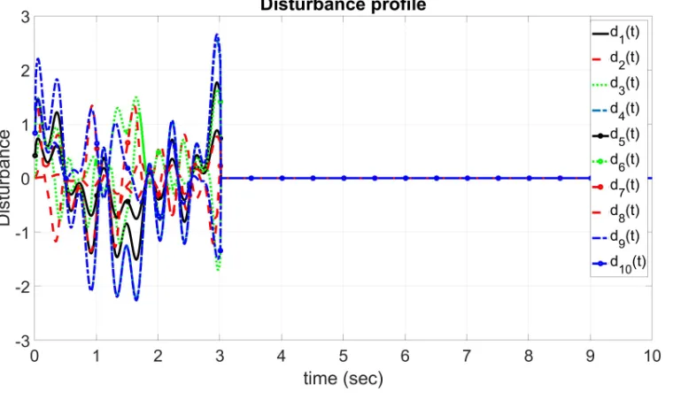
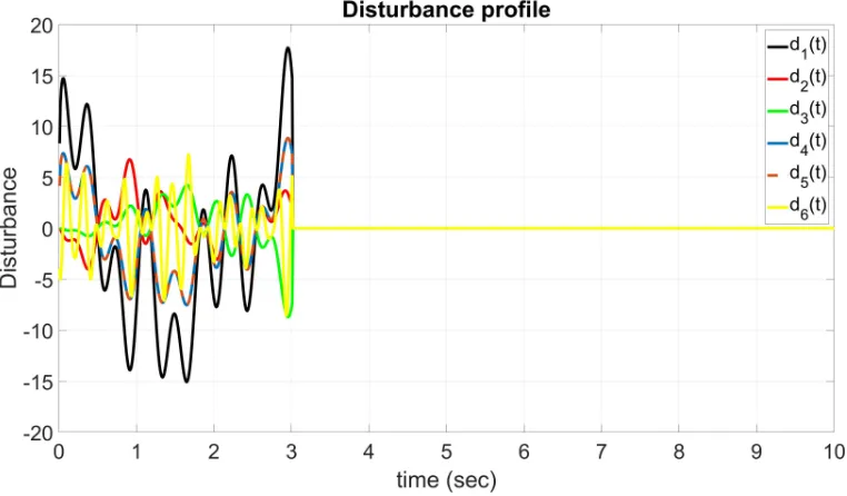
Figure 3.8 Disturbance profile. . . 64
Figure 3.9 State consensus under disturbance with output-feedback protocol. . . 65
Figure 3.10 Controlled output profile with output-feedback protocol. . . 66
Figure 3.11 Controlled output profile for 30 agents with weighted Laplacian matrix. . . 69
Figure 3.12 Disturbance profile . . . 70
Figure 3.13 State consensus under disturbance . . . 71
Figure 3.14 Controlled output profile. . . 72
Figure 3.15 Network graph of ten agents . . . 72
Figure 3.16 closed-loop poles location for 10 agents with vertical band[−10,−0.1]. . . 73
Figure 3.17 Disturbance profile with 10 agents . . . 74
Figure 3.18 Controlled output profile for 10 agents. . . 75
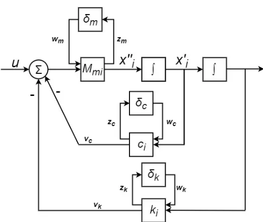
Figure 4.1 Block diagram of uncertain mass-spring-damper systems . . . 110
Figure 4.2 LFT form ofmi . . . 111
Figure 4.3 LFT form ofciandki . . . 111
Figure 4.4 LFT representation of uncertain mass-spring-damper systems . . . 112
Figure 4.5 Input/output block diagram of the mass-damper-spring system. . . 113
Figure 4.6 Undirected network graph of six interconnected agents. . . 114
Figure 4.7 Disturbance profile . . . 116
Figure 4.8 State consensus under disturbance with state-feedback protocol. . . 117
Figure 4.9 Controlled output profile with state-feedback protocol. . . 118
Figure 4.10 Disturbance profile. . . 119
Figure 4.11 State consensus under disturbance with output-feedback protocol. . . 120
Figure 4.12 Controlled output profile with output-feedback protocol. . . 121
Figure 4.13 Network graph of ten agents . . . 122
Figure 4.14 Disturbance profile with 10 agents . . . 124
Figure 4.16 Controlled output profile for 10 agents. . . 126
Figure 4.17 Network graph of six interconnected agents. . . 126
Figure 4.18 Large-scale consensus under disturbance with output-feedback protocol. . . . 128
Figure 4.19 Controlled output profile for 10 agents. . . 129
Figure 5.1 Undirected network graph of six interconnected agents. . . 148
Figure 5.2 Disturbance profile . . . 149
Figure 5.3 State consensus under disturbance with node-base protocol. . . 150
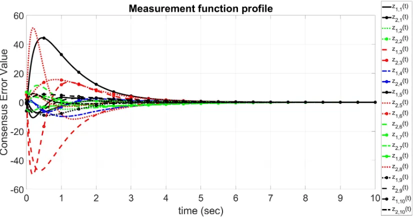
Figure 5.4 Consensus error profile with node-base protocol. . . 151
Figure 5.5 Coupling weights for each node profile. . . 151
Figure 5.6 State consensus under disturbance with edge-base protocol. . . 153
Figure 5.7 Consensus error profile with edge-base protocol. . . 154
Figure 5.8 Coupling weights for each edge profile. . . 154
Figure 5.9 Switching Network graphG1andG2. . . 155
Figure 5.10 Switching information versus time. . . 155
Figure 5.11 State consensus under disturbance and switching graph . . . 156
Figure 5.12 Consensus error profile with switching graph. . . 157
LIST OF SYMBOLS
Mathematical Symbols
R Set of real numbers
R+ Set of non-negative real numbers
Rn Set ofn-dimensional real vectors Rm×n Set of realm×nmatrices
Sn×n Set of symmetric matrices inRn×n Sn+×n Set of positive definite matrices inRn×n
In n×nIdentity matrix;also denoted asI if the dimension is clear from the context 0m×n n×nIdentity matrix;also denoted asI if the dimension is clear from the context
1n n- dimensional column vector with all elements being 1
diag{X1,X2,· · ·,Xn} A block diagonal matrix with matricesX1,X2,· · ·,Xpon its main diagonal A⊗B Kronecker product of matricesAandB
col{x1,x2,· · ·,xn} A column vectors by stackingx1,x2,· · ·,xntogether ? Entries in LMIs that follow from symmetry
MT the transpose of the matrixM
M−1 the inverse of the invertible matrixM
M∗ the conjugate transpose transpose of the matrixM
M >0(M ≥0) the matrixM is positive definite (positive semi-definite) M <0(M ≤0) the matrixM is is negative definite (negative semi-definite)
L2 space of square integrable functions λi(M) ith eigenvalue ofM
Symbols for Graph Theory
D directed graph
V vertex set;if necessary, denoted byV(G)orV(D) E vertex set;if necessary, denoted byE(G)orE(D)
ei j= (vi,vj) edge in a graph; also denoted byvivj ori j N(i) set of agents adjacent toi
∆(G) degree matrix of graphG
A(G) adjacency matrix of graphG
D(G) incidence matrix of graphG L(G) graph nominal Laplacian ofG Le(G) graph edge-weighted Laplacian ofG
CHAPTER
1
INTRODUCTION
1.1
Background
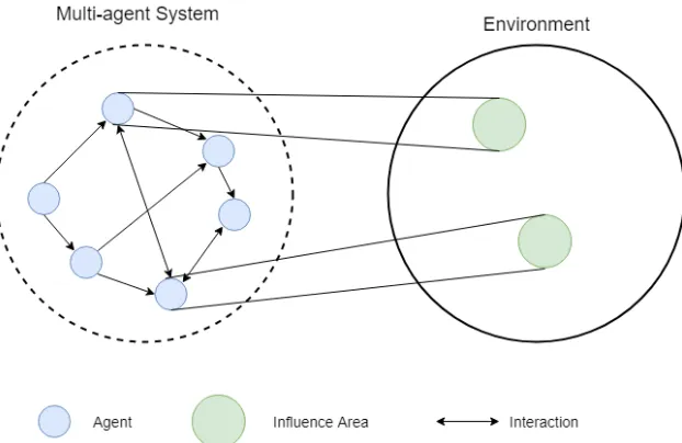
With the development of sensor technology, information communication technique and the modern control theory, control of multi-agent systems and their coordinated movement has attracted many research interests because of its various applications in engineering and modern industry, such as formation control, rendezvous, attitude alignment, flocking, foraging, task and role assignment, payload transport and air traffic control[72]. Better operational capability and efficiency can be achieved from multi-agent systems in a coordinated fashion in comparison to a single agent. By using multi-agent systems, global objectives can be achieved through sensing, exchange of information using communication and control[108]. Difficulties in modeling and computation can be organized as subsystems and/or agents. A multi-agent system is a computerized system composed of multiple interacting intelligent agents, which can interact with each other through communication as shown in Fig. 1.1.
Figure 1.1Diagram of multi-agent systems with six agents.
its own controller, which utilizes the local information from itself and/or its neighbors. Compared to the centralized approach, the distributed control of multi-agent systems has greater efficiency due to many physical constraints such as limited resources and energy, short wireless communication ranges, narrow bandwidths, and large sizes of vehicles to manage and control[6]. Moreover, the distributed control approach offers greater robustness and flexibility to realistic circumstances since the damage of a few agents doesn’t affect achievement of the goal for the whole system.
Figure 1.2Diagram of a centralized approach.
Figure 1.3Diagram of a distributed approach.
control in the field of control systems including: consensus[55, 62, 74], distributed formation[36, 61], distributed optimization[7, 67]and distributed estimation[5, 109, 102, 10, 54, 103, 81].
As one of the important problems, consensus of multi-agent systems means that the states of agents reach an agreement based on the relative information of each agent. The word "relative" means agents can only obtain the information related to each other instead of the absolute states. Consensus of multi-agent systems can be achieved by utilizing the consensus algorithms and local distributed protocol. Various applications benefit from consensus control including rendezvous[46, 47, 57], formation control[13, 34, 49, 32, 68], flocking[62, 84, 89, 12, 59, 35], attitude alignment[33, 73, 69], and sensor networks[97, 82, 63, 15]. As a result, the study of consensus control has received growing attention in recent years.
However, the consensus control of multi-agent systems presents many challenges to the control designers. Briefly speaking, a consensus protocol design is desired to address the following problems: • It is often difficult to obtain the states of all agents due to economic reasons and limitations
on measurements.
• With the increasing size of multi-agent systems, it is necessary to provide a tractable distributed control design approach with less conservatism and computational efficiency.
• Achieving consensus for multi-agent systems with both general class of uncertainty descrip-tion and external disturbance remains an open problem in the field.
1.2
Objectives
This dissertation will provide systematic and optimized distributed control design strategies to the problem of multi-agent systems with dynamic uncertainty and unknown external disturbance. Specifically, we will aim at the following consensus problems:
• For the general linear multi-agent systems subject to unknown external disturbances, a dis-tributed dynamic output-feedback control protocol design for solvingH∞consensus problem and convexified consensus synthesis will be proposed.
• For the general linear multi-agent systems subject to unknown external disturbances and structured uncertainties, two types of consensus protocols, namely state feedback control protocol and output-feedback protocol, for solving robustH∞consensus problem will be studied.
• For the general linear multi-agent systems subject to unknown external disturbances, two types of fully distributed adaptive consensus protocols, a node-based protocol and an edge-based protocol, for solvingH∞consensus problem and convexified consensus synthesis will be investigated.
1.3
Overview of related work
1.3.1 Consensus Control
Consensus refers to the group behavior that all the agents asymptotically reach a certain common agreement through a local distributed protocol[6]. The basic idea of a consensus algorithm is to impose similar dynamics on the information states of each agent. If the communication network among vehicles allows continuous communication, then the information state update of each agent is modeled using a differential equation[72]. Some pioneer works about the algorithm can be found in[75]and[27].
a Laplacian matrix is the algebraic connectivity, which represents the convergence rate of consensus algorithms[31]. Details about graph theory will be presented in the next chapter.
From graph theory, consensus control problem was studied in three main directions, which are dynamic of agents, control architectures, and network communications[26]. The dynamic of agents can be organized into three groups, which are single integrator dynamics, double integrator dynamics and high-order dynamics. The early work on consensus problem has mainly focused on integrator dynamics, such as single-integrator[3, 70, 74, 62, 27], double-order integrator[71, 98, 16]and higher-order[66, 87, 41, 76, 78, 110, 65, 24]. Specifically,[3]studied average consensus problems for undirected networks of dynamic agents having communication delays. In[70], the consensus problem of the information states of all agents approaching a time-varying reference state was investigated.[74, 98, 16]considered the problem of information consensus among multiple agents in the presence of limited and unreliable information exchange with dynamically changing interaction topologies.[62]proposed consensus problems for a network of single integrator dynamic agents with fixed and switching topologies. Then the extension to double integrator models has been considered in[71]. The average-consensus problem for networks of double-order integrator dynamic agents was investigated in[98].[16]considered a group of agents communicating through an undirected and weighted network towards a consensus point.
Since the practical complex systems can be hardly described or linearized as single integrator or double integrator dynamic, the study has shifted to multi-agent systems with general linear dynamics.[66]introduced the framework that to analyze and design cooperative controls for a group of individual dynamical systems.[87]presented the conditions for synchronizability in arrays of coupled linear system.[41]addressed the consensus problem of multi agent systems with a time-invariant communication topology consisting of general linear node dynamics. Synchronization of a network of identical linear state-space models under a possibly time-varying and directed interconnection structure was investigated in[76].[78]showed the consensus problem for multi-agent linear dynamic systems, which all the multi-agents have identical MIMO linear dynamics that can be of any order.
convex problem in term of Lyapunov matrix and static controller gain. Although computational methods based on iterative solutions of the two convex LMI problems with respect to Lyapunov matrix and its inverse have been proposed to find stabilizing static output-feedback gains, but convergence of the iterative algorithms is not guaranteed.
In addition, observer-type consensus protocols were introduced in[39, 114, 14]. An observer-type consensus protocol based on the relative outputs of the neighboring agents was adopted in[39] [114] studied multi-agent systems with time delays in both the communication network and inputs by observer-based output-feedback protocols.[14]characterized necessary and sufficient conditions for consensus of agents under distributed observer-based output-feedback control. However, it should be noted that the protocols of observer-type require an estimate of the system state.[51, 92, 1]presented dynamic output feedback protocols to achieveH∞consensus. A distributed dynamic output-feedback protocol was proposed in[51]to solve theH∞consensus problem.[92]investigated theH∞consensus problem for networks of multi-agent systems subject to external disturbances. In particular, a distributed dynamic output-feedback controller with time-varying delays was provided. Nevertheless, the synthesis conditions assume decoupled structure of the Lyapunov matrix, which is conservative and cannot achieve minimalL2gain performance. Essentially, the protocols in[51, 92, 1]are combinations of state feedback protocol and observer-type protocol. On the other hand, [111]solved the consensus problem via general dynamic output-feedback, the resulting synthesis conditions are however formulated as bilinear matrix inequalities (BMIs), which are difficult to solve.
It should be noted that the topic of distributed output-feedback consensus control for leader-following multi-agent systems (see[106]and references therein) is different from the leaderless topic. Specifically, for leader-following consensus, the output-feedback synthesis problem can be easily formulated as convex conditions. But when it comes to leaderless consensus, the problem becomes very challenging. Conventional dynamic output-feedback leaderless consensus algorithms often lead to non-convex synthesis conditions[111]. Therefore, developing computationally tractable and performance optimized output-feedback control synthesis conditions for leaderless multi-agent systems remains as an open problem in the field.
1.3.2 Uncertainties and disturbances in multi-agent systems
the multi-agent systems with addictive dynamic uncertainties under a dynamic output-feedback protocol of the observer-based type were studied in[38].[85]considered uncertainty in the form of additive perturbations of the transfer matrices of the nominal dynamics. References[48, 52, 92, 43, 25]considered parametric uncertainties of linear multi-agent systems.[52]was devoted to the robustH∞consensus control of multi-agent systems with model parameter uncertainties. In[92], consensus problem was discussed for a class of multi agent systems with parameter uncertain-ties under a fixed directed graph. Mixed uncertainuncertain-ties were investigated in[25]. The robustness to external disturbance was also investigated in[83, 52, 53].
Consensus problems of multi-agent systems under uncertainties and external disturbances were reformulated as robustH∞consensus problem. With the help ofH∞techniques, sufficient conditions are given to achieve the robust consensus with prescribedH∞performance, and the proposed consensus protocol is obtained[53]. Some related literature were presented in[42, 48, 53, 51, 52]. The disturbance rejection problem in multi-agent system arisen in[42]. The agent network is said to possess a desired level of disturbance rejection, if theH∞norm of its transfer function matrix from the disturbance to the controlled output is satisfactorily small. The consensus prob-lems for directed networks of first-order agents with external disturbances and model uncertainty was studied in[48]. It proved that the problem could be transformed into a robustH∞control problem. The consensus control of general linear multi-agent systems with state and measurement disturbances were proposed in[53, 51].[52]was devoted to the robustH∞consensus control of multi-agent systems with model parameter uncertainties and external disturbances. In particu-lar, networks of multiple agents with general linear dynamics under uncertain communication delays were considered. Generally speaking, to solve the robustH∞consensus problem, the model of multi-agent systems will be transformed to an equivalent reduced-order system regarding the
H∞performance. Then the reduced-order system converts to a set of independent linear systems described by a single agent. Finally, the consensus problem can be determined by robust control techniques.
1.3.3 Communication in multi-agent systems
The network communications describe the approach that the agents interact with each other. The interaction between agents can be characterized by the graph Laplacian matrix[79]. The graph Laplacian can be specified into different categories, like fixed[94, 60, 93, 92]and switching[60, 62, 53, 52]Laplacian, or undirected[113, 104, 43]and directed graph. The Laplacian matrix is a constant matrix in the fixed graph and a time-varying matrix in the switching graph. Note that the undirected graph is a special case of directed graph. The details about Laplacian graph will be introduced in the next chapter.
It should be noted that the robust consensus protocols in[52, 92, 43]were applicable to only undirected graphs or balanced directed graphs. The robust consensus problem under undirected graphs or balanced directed graph is different from the unbalanced graph. Specifically, for consensus problem under undirected graphs or balanced directed graph, the multi-agent systems can be easily decoupled with orthogonal transformation. But when it comes to unbalanced directed consensus, the problem becomes very challenging because the Laplacian matrices of directed graphs are generally asymmetric, which renders the decoupling of the multi-agent systems a far from being easy.
One common feature in the aforementioned research is that the consensus protocols require information of nonzero eigenvalues of the Laplacian matrix associated with the communication graph. However, the nonzero eigenvalue of the Laplacian matrix is global information that cannot be acquired by the agents in the fully distributed implementation, which means using only the local information of its own and neighbors. To overcome the limitation, distributed full state adaptive consensus protocols have been proposed in[44, 40, 17]. Specifically, distributed relative-state consensus protocols with an adaptive law for adjusting the coupling weights between neighboring agents were designed in[44]for general linear and Lipschitz nonlinear dynamics. Full state consensus node and edge protocols with adaptive gains of general linear dynamics multi agent systems subject to bounded external disturbances was investigated in[40].[17]considered the consensus problem of multi-agent systems with matched disturbances. Distributed adaptive protocols were proposed, which rely on the state information of neighbor agents. Note that the protocols in[44, 40, 17]rely on all relative states information of neighboring agents, which is difficult to obtain due to economic reasons and limitations on state measurements.
[45, 28]are restrictive in the following aspects. Firstly, the synthesis conditions used structured Lyapunov matrix, which is conservative in achieving minimalL2gain performance. Secondly, the
H∞norm in[28]is represented by three indices, which cannot be solved by minimal optimization problem. Thirdly, necessary and sufficient conditions for the existence of consensus protocols in[28] is actually the necessary conditions only. The sufficiency conditions need to be verified after solving the Lyapunov matrix. Therefore, there are few works focusing on convex solutions for adaptive multi-agent output-feedback consensus.
1.4
Contributions
Major contributions of the dissertation can be summarized as follows:
• A novel distributed dynamic output-feedback protocol, which utilizes not only relative mea-surement output information but also relative state information of neighboring controllers, is designed for general linear multi-agent systems under unknown external disturbance and structured uncertainties.
• Convexified synthesis conditions for multi-agent under unknown external disturbance is established in an LMI form without introducing additional conservatism to optimize the novel distributed dynamic output-feedback protocol.
• Synthesis condition for multi-agent consensus using state-feedback control is established in terms of LMIs. Meanwhile, synthesis condition for multi-agent consensus using output-feedback control is established in terms of BMIs without introducing any conservatism from analysis condition, which can be used to optimize the proposed distributed control protocol via an iterative algorithm.
• Two types of novel fully distributed adaptive dynamic output-feedback adaptive protocols are designed for linear multi-agent systems under unknown external disturbance. With the help of such novel structure of consensus protocols, the Lyapunov matrix can be assumed as a general form without introducing restriction.
• Convexified synthesis condition for multi-agent output-feedback adaptive consensus con-trol in an LMI form is derived without introducing additional conservatism. The synthesis conditions are unified for both node-based and edge-based adaptive protocols.
1.5
Outlines
The detailed outline of this dissertation is as follows:
Chapter 1 introduces the background of multi-agent systems and distributed control, the aim of the research. Then some related works, which include consensus control, uncertainties, disturbances and communication in multi-agent systems, are reviewed. Finally, the major contributions of the dissertation are summarized.
Chapter 2 presents some preliminaries of consensus control, which covers the mathematical background and definition, graph theory and some definitions and theorems about stability theory.
Chapter 3 investigates theH∞consensus problem for general linear multi-agent systems subject to external disturbances. A novel distributed dynamic output-feedback controller will be proposed. Through model transformation, theH∞consensus control problem of multi-agents network is reduced to a set of independentH∞stabilization sub-problems forn-dimensional linear sys-tems. Sufficient analysis conditions are derived using Lyapunov method. TheH∞output-feedback consensus synthesis conditions are convexified without introducing additional conservatism and formulated as linear matrix inequalities, which can be solved efficiently via convex optimization. Moreover, the consensus value analysis,H∞consensus synthesis with pole placement and Lapla-cian spectral constraint for synthesis conditions will be also presented in chapter 3.
time-varying coupling weight to each edge in the communication graph. The proposed protocols utilize relative output information of neighboring agents and relative state information of neigh-boring controllers, which are in a fully distributed fashion. With the help of such novel structures of consensus protocol and congruent transformation, we will be able to derive the linear matrix inequality (LMI) conditions for multi-agent adaptive output-feedback control in distributed manor. The adaptiveH∞consensus under the switching graph is also introduced in this chapter.
CHAPTER
2
PRELIMINARIES OF CONSENSUS
CONTROL
2.1
Mathematical Preliminaries
Some mathematical theory, basic notation and definition will be introduced in this section for further use in the thesis.
Kronecker Product
Kronecker Product[23]is defined for two matrices of arbitrary size. In the consensus control of the multi-agent systems, it is used to describe the connection of the networks.
Definition 2.1. If there exists a matrix A∈Rm×n and matrix B∈Rp×q, then the Kronecker product A⊗B is defined as
A⊗B=
a11B · · · a1nB ..
. ... ... am1B · · · am nB
∈R
m p×n q
• A⊗(B+C) =A⊗B+A⊗C
• (A+B)⊗C =A⊗C+B⊗C
• (k A)⊗B=A⊗(k B) =k(A⊗B)
• (A⊗B)⊗C =A⊗(B⊗C)
• (A⊗B)(C ⊗D) = (AC)⊗(B D)
• (A⊗B)−1=A−1⊗B−1
• (A⊗B)T =AT⊗BT and(A⊗B)∗=A∗⊗B∗
• If A and B are both positive definite (semi-positive definite), so is A⊗B .
where A, B , C and D are matrices with compatible dimension, k is scalar.
Eigenvalues and Eigenvectors
Eigenvalues and eigenvectors have their importance in the design of consensus control because the eigenvalues of Laplacian matrix are required. The definition of eigenvalues and eigenvectors[50]is given as:
Definition 2.2. Let A be a square matrix A∈Rn×n. A scalarλis called an eigenvalue of A if there exists a nonzero (column) vector v such that
Av=λv
Any vector satisfying this relation is called an eigenvector of A belonging to the eigenvalueλ.
In engineering and stability theory, a square matrixA∈Rn×nis called a Hurwitz matrix[30](or sometimes a stable matrix) if every eigenvalueλiofAhas strictly negative real part, that is,
Re(λi)<0.
Gershgorin Disc Theorem
Lemma 2.1. Let A= [ai j]∈Rn×n, and let
Ri0(A) = n
X
j=1,j6=i
ai j
, 1≤i≤n
denotes the deleted absolute row sums of A. Then all the eigenvalues of A are located in the union of n discs
G(A)≡
n
[
i=1
z∈C:|z−ai i| ≤Ri0(A)
Furthermore, if a union of k of these n discs forms a connected region that is disjoint from all remaining n−k discs, then there are precisely k eigenvalues of A in this region.
Schur Complement Lemma
A nonlinear convex inequalities can be presented as LMI form using Schur complements[4]. The basic idea is as follows:
Lemma 2.2. Let S be a symmetric matrix of the partitioned form that
S= [Si j] =
S11 S12 ST
12 S22
with S11∈Rr×r, S12∈Rr×(n−r)and S22∈R(n−r)×(n−r). Then the following statements are equivalent: • S<0.
• S11<0, S22−S21S−1 11S12<0. • S22<0, S11−S12S−1
22S21<0. Hilbert space
A Hilbert space[115]is a complete inner product space with the norm induced by its inner product. For example,Cnwith the usual inner product is a (finite-dimensional) Hilbert space. More generally, it is straightforward to verify thatCn×m with the inner product defined as
〈A,B〉:=traceA∗B= n
X
i=1 m
X
j=1 ¯
ai jbi j ∀A,B∈Cn×m
A well-know infinite-dimensional Hilbert space isL2[a,b], which consists of all square integrable and Lebesgue measurable functions defined on an interval[a,b]with the inner product defined as
f,g:=
Z b
a
f(t)∗g(t)d t
forf,g ∈ L2[a,b]. Similarly, if the functions are vector or matrix-valued, the inner product is defined correspondingly as
f,g:=
Z b
a
trace[f(t)∗g(t)]d t
Some spaces used often in this book areL2[0,∞),L2(−∞, 0],L2(−∞,∞), More precisely, they are defined as
• L2=L2(−∞,∞): Hilbert space of matrix-valued functions onR, with inner product
f,g:=
Z ∞
−∞
f(t)∗g(t)d t
• L2+=L2[0,∞): subspace ofL2(−∞,∞)with functions zero fort <0. • L2−=L2(−∞, 0]: subspace ofL2(−∞,∞)with functions zero fort >0.
Linear Fractional Transformations
Linear Fractional Transformations (LFT) is a powerful and flexible tool in modern and robust control theory. It is naturally related to feedback interconnection and provides a systematic approach in representing uncertainty. For a complex matrixM, relatingr andv throughv=M r. Partition into top and bottom, we have
v1=M11r1+M12r2 v2=M21r1+M22r2
Matrix∆relatingv2tor2asr2=∆v2. The linear fractional transformation (LFT) ofM by∆ Eliminatev2andr2leaving
Figure 2.1The lower linear fractional transformation
Figure 2.2The upper linear fractional transformation
v2= [M22+M21Ω(I−M11∆)−1M12]r2=:FU(M,Ω)r2
2.2
Graph Theory
In this section, the fundamental concept of graph theory is introduced. Algebraic graph theory plays an important role in describing the communication topology of multi-agent system. The material in this section is from[58, 72].
2.2.1 Fundamental of Graphs
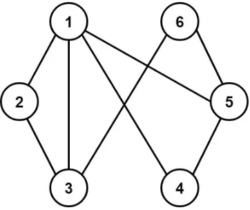
The graph identifies agents withnodesin a graph and encodes the existence of an interaction between nodes asedges. The interaction graph plays an important role in the analysis and synthesis of the networked multi-agent systems regardless of whether the information exchange takes place over a communication network or though active sensing. For example, as shown in Fig.2.3, a network of four agents can be viewed as a graph, with four nodes corresponding to the agents and four edges to the interactions.
Suppose that a multi-agent system consists ofnagents. A directed graph of ordernis defined as
Figure 2.3A network of four agents represented by nodes and edges in the graph theory
of ordered pairs of nodes. The edge set consists of elements of the form(i,j), wherei,j=1, 2,· · ·,n andi6=j. The edge(i,j)in the edge set denotes that agentj can receive information from agent i, but not necessarily vice versa. For the edge(i,j),i is the parent mode and j is the child node. If(i,j)∈ E, we said nodei is a neighbor of nodej. The set of neighbors of nodei is denoted as
Ni. Contrary to a directed graph, the pairs of nodes in an undirected graph are unordered. The edge(i,j)in undirected graph denotes that agentj and agenti can obtain information from each other. Therefore, an undirected graph is a special case of a directed graph with an edge(i,j)in an undirected graph corresponds to edges(i,j)and(j,i)in a directed graph. Fig. 2.4 provides an example of an undirected graphG= (V,E)with the node setV :={v1,v2,v3,v4,v5}and the edge set
E ⊆ V × V ={v1v2,v2v3,v3v4,v3v5,v2v5,v4v5}.
Figure 2.4An undirected graphG= (V,E)with 5 agents
2.2.2 Matrix Representation of Graphs
In graph theory, a multi-agent systems not only can be graphically represented by nodes and edges, but also expressed in term of matrices. In this section, some important matrices in graph theory will be introduced.
Adjacency and Degree matrices
For the graphG = (V,E), the degree of the nodesd(vi)is the cardinality of the neighbors setNiand is equal to the number of nodes that are adjacent to nodevi. The degree matrix∆(G)is a diagonal matrix with the degree of the nodes as the diagonal elements, which is
[∆(G)]i j=
¨
d(vi) i=j 0 i6=j Therefore, the degree matrix∆(G)for the graph shown in Fig. 2.4 is
∆(G) =
1 0 0 0 0
0 3 0 0 0
0 0 3 0 0
0 0 0 2 0
0 0 0 0 3
The adjacency matrixA(G)is an×nmatrix, which describes the adjacency relationships in graph
G, that is
[A(G)]i j=ai j=
¨
postive weight ifvivj∈ E 0 otherwise
If the weights are not relevant or the graphs are unweighted, thenai jis set equal to 1 for all(j,i)∈ E. A graph is called balanced ifPn
j=1ai j=
Pn
matrix is:
A(G) =
0 1 0 0 0
1 0 1 0 1
0 1 0 1 1
0 0 1 0 1
0 1 1 1 0
Incidence Matrix
For an undirected graphG(V,E)withnnodes andmedges, the incidence matrixD(G)∈Rn×m is defined as
[D(G)]i j=di j =
−1 ifviis the tail ofej, 1 ifviis the head ofej, 0 otherwise.
Note that the incidence matrixD(G)is neither unique for an undirected graph nor changed by the orientation of the graph. The incidence matrixD(G)for the graph shown in Fig. 2.4 is
D(G) =
1 0 0 0 0 0
−1 1 0 0 1 0
0 −1 1 0 0 1
0 0 −1 1 0 0
0 0 0 −1 −1 −1
As can be seen from this example, this incidence matrix has a column sum equal to zero, which is a fact that holds for all incidence matrices since every edge has to have exactly one tail and one head.
Nominal Laplacian matrices
Nominal Laplacian matrixL(G)is another matrix representation of graphG. There are several ways to define nominal Laplacian matrixL (henceforth Laplacian matrix). The first definition of the graph Laplacian associated with a graphG is
where∆(G)is the degree matrix andA(G)is the adjacency matrix. An alternative way to define Laplacian matrixL(G)is
[L(G)]i j=
¨ PN
j=1,j6=iai j i=j
−ai j i6=j
The Laplacian matrixL(G)can also be represented by the incidence matrixD(G)as
L(G) =D(G)D(G)T
Hence, the Laplacian matrix associated with the graphG in Fig. 2.4 is
L(G) =
1 −1 0 0 0
−1 3 −1 0 −1
0 −1 3 −1 −1
0 0 −1 2 −1
0 −1 −1 −1 3
Laplacian matrixLhas the following important properties[13, 72]in consensus protocol design. • For an undirected graph,Lis symmetric. For a directed graph,Lis not necessarily symmetric. • Since Laplacian matrixLhas zero row sums, 0 is an eigenvalue ofL associated with
eigen-vector1N.
• L is diagonally dominant and has non-negative diagonal entries.
• According to Gershgorin disc theorem[22], for an undirected graph, all nonzero eigenvalues ofL are positive, whereas, for a directed graph, all of the nonzero eigenvalues ofL have positive real parts. Therefore, all of the nonzero eigenvalues of−L have negative real parts. • For an undirected graph, 0 is a simple eigenvalue ofL if and only if the undirected graph is
connected. For a directed graph, 0 is a simple eigenvalue ofL if the directed graph is strongly connected.
• For an undirected graph, setλiLbe theith smallest eigenvalue ofL withλ1(L)≤λ2(L)≤
Graph weighted Laplacian
Together with the edge and node sets, functionsk :E →Randm:V →Rare given that associate a value to each edge and node, respectively. Then one can form the edge-weighted LaplacianLe as
Le=D(L)K D(L)T
and the node- and edge-weighted Laplacian (henceforth weighted Laplacian)Lg as
Lg=M−1D(L)K D(L)T
WhereK 0 is anm×mdiagonal edge weighting matrix, withk(ei),i=1,· · ·,m, the edge weight for each edge on the diagonal andM 0 is ann×ndiagonal edge weighting matrix, withm(vi),i= 1,· · ·,n, the node weight for each node on the diagonal.
The edge-weighted Laplacian Le has some similar properties to the nominal LaplacianL proposed in[79]:
• The matricesL andLe are symmetric positive semidefinite, with at least one eigenvalue at zero corresponding to an eigenvector1n= (1/
p
n)[1· · ·1]T.
• If the graph represented byL orLe is connected, thenL orLe , respectively, has exactly one eigenvalue at zero.
AlthoughLg is not symmetric in general, its eigenvalues possess properties similar to those ofL or
Le
Lemma 2.3. [79]Every eigenvalue ofLg=M D(L)K D(L)T is real and non-negative. IfLgrepresents a connected graph, then all eigenvalues ofLg, excepting one at zero, are positive.
The edge-weighted LaplacianLe and weighted LaplacianLg are important in the Laplacian spectral constrains design. The details will be introduced in Chapter 3.
2.3
Stability theory
Stability theory plays an essential role in control systems. In this thesis, Lyapunov stability theory, which focuses on the stability of equilibrium points, is used to determine the stability of dynamic systems. In this section, some basic definitions and theorems will be introduced. The material in this section is mainly from[30].
Consider the nonlinear system
˙
where f :D →Rn is a locally Lipschitz map from a domain D ⊂Rn intoRn. Suppose ¯x is an equilibrium point of (2.1); that is, f(x¯) =0. There is no loss of generality in doing so because any equilibrium point can be shifted to the origin via a change of variables. Therefore, we will always assume that f(x)satisfies f(0) =0 and study the stability of the originx =0. The definition of stability will be stated in the following.
Definition 2.3. The equilibrium point x =0of (2.1) is • stable if, for each" >0, there isδ=δ(")>0such that
kx(0)k< δ⇒ kx(t)k< ",∀t ≥0
• unstable if it is not stable
• asymptotically stable if it is stable andδcan be chosen such that
kx(0)k< δ⇒ lim
t→∞x(t) =0
Lyapunov stability
Having defined stability and asymptotic stability of equilibrium points, Lyapunov stability theorem [30]gives an approach to determine stability.
Theorem 2.1. Let x=0be an equilibrium point for (2.1) and D⊂Rnbe a domain containing x=0. Let V :D→R be a continuously differentiable function, such that
V(0) =0 and V(x)>0 inD− {0} (2.2) ˙
V(x)≤0 inD (2.3)
Then, x=0is stable. Moreover, if
˙
V(x)<0 inD− {0} (2.4)
then x=0is asymptotically stable.
A continuously differentiable functionV(x)satisfying (2.2) is called a Lyapunov function. The surfaceV(x) =c, for somec>0, is called a Lyapunov surface. A functionV(x)satisfying condition (2.2) is said to be positive definite. If it satisfies the weaker conditionV(x)≥0 forx6=0, it is said to be positive semi-definite. A functionV(x)is said to be negative definite or negative semi-definite if
The Invariance Principle
From Lyapunov stability Theorem 2.1 we know thatx=0 is asymptotically stable if the derivative of Lyapunov function ˙V(x)is negative definite. While the derivative of Lyapunov function ˙V(x)is semi-negative definite, the asymptotically stable is not guaranteed. However, this problem can be if we can find ˙V(x)≤0 and no trajectory can stay at points where ˙V(x) =0 except at thex=0. Then asymptotically stable ofx=0 is achieved. LaSalle’s theorem[30]is used to prove the asymptotically stable under ˙V(x)≤0.
Theorem 2.2. [30]LetΩ⊂D be a compact set that is positively invariant with respect to (2.1). Let V :D→Rbe a continuously differentiable function such thatV˙(x)≤0inΩ. Let E be the set of all points inΩwhereV˙(x) =0. Let M be the largest invariant set in E . Then every solution starting inΩ approached M as t→ ∞.
Different from the Lyapunov stability Theorem 2.1, LaSalle’s Theorem 2.2 doesn’t require the functionV(x)to be positive definite. When our interest is in showing thatx(t)→0 ast → ∞, we need to establish that the largest invariant set inE is the origin. This is done by showing that no solution can stay identically inE, other than the trivial solutionx(t)≡0. We obtain the following two corollaries that extend Theorem 2.1 and 2.2.
Corollary 2.1. Let x=0be equilibrium point for (2.1). Let V :D→Rbe a continuously differentiable function on a domain D containing the origin x=0, such thatV˙(x)≤0in D . Let S=x∈D|V˙(x) =0 and suppose that no solution can stay identically in S , other than the trivial solution x(t)≡0. Then, the origin is asymptotically stable.
CHAPTER
3
CONSENSUS CONTROL FOR
MULTI-AGENT SYSTEMS WITH
EXTERNAL DISTURBANCES
3.1
Introduction
In this chapter, we investigate theH∞consensus problem for general linear multi-agent systems subject to external disturbances. The objective of this chapter is to design a distributed output-feedback protocol of multi-agent systems to solve theH∞consensus control problem.
A novel distributed dynamic output feedback controller will be proposed. Through model transformation, theH∞consensus control problem of multi-agents network is reduced to a set of independentH∞stabilization sub-problems forn-dimensional linear systems. Sufficient analysis conditions are derived using Lyapunov method and theH∞output-feedback consensus synthesis conditions are convexified without introducing additional conservatism and formulated as linear matrix inequalities, which can be solved efficiently via convex optimization. Moreover, the consensus value analysis andH∞consensus synthesis with pole placement will be also presented in this chapter.
of neighboring agents but also relative state information of neighboring controllers. With the help of such a novel structure of consensus protocol and congruent transformation, we will be able to derive the linear matrix inequality (LMI) conditions for multi-agent output feedback control.
The rest of this chapter is organized as follows. The problem statement and objective are rep-resented in Section 3.2. The novel distributed dynamic output feedback control protocol,H∞ consensus analysis, synthesis conditions and consensus values are studied in sections 3.3. Section 3.4 extends theH∞consensus to the unbalanced directed graph. Section 3.5 introduces the defini-tion of LMI regions and its applicadefini-tion to multi-agent systems. The effectiveness of the proposed protocol is demonstrated by two numerical examples in section 3.7. Finally, the chapter concludes in section 3.8.
3.2
Problem statement
3.2.1 Model description
Consider a multi-agent system consisting ofN dynamic agents with identical linear dynamics subject to external disturbance
˙
xi=A xi+B1di+B2ui yi=C xi+D di
, (3.1)
wherexi∈Rnis each agent’s state,di∈Rn1is the external disturbance applied toith agent,y
i∈Rm represents the measured output andui∈Rn2represents the control input for the agenti. All matrices
in eqn. (3.1) are known real constant matrices of appropriate dimensions. Without loss of generality, B2is assumed of full column rank.
Some assumptions are needed for system matrices and the network graphG associated the multi-agent system (3.1).
Assumption 3.1. The associated network graphGis undirected and connected.
Assumption 3.2. For the system matrices in (3.1),(A,B2)is stabilizable and(A,C)is detectable.
Remark 3.1. The assumption that B2is of full column rank is made without loss of generality for the multi-agent systems (3.1). If the matrix B2in (3.1) is not of full column rank, we can still develop an equivalent model satisfying full column rank conditions of B2and use it for controller design. Detailed explanations are given below.
Consider matrix B2∈Rn×n2 is of rank l and is not of full column rank. A singular value
andB¯2is given by
¯ B2=
Σl 0l×(n2−l)
0(n−l)×l 0(n−l)×(n2−l)
WhereΣl ∈Rl×l is a diagonal matrix with entries of the singular value of B2. Define u¯ =
¯ u1
¯ u2
= V u , where u represents the control input and u¯1 ∈ Rl. Then consider a
full column rank matrixBˆ2=U
Σl
0(n−l)×l
∈Rn×l. It follows that B2u(t) =Bˆ2u¯1(t). Therefore the B2u(t)can be replaced withBˆ2u¯1(t)in the design of the controller. We can observe thatu¯2(t)has no contribution to B2u(t)henceu¯2(t)can be chosen arbitrarily and set to be a zero vector. The actual control input can be obtained as u(t) =V−1
Σl
0(n2−l)×1
. Therefore there is no loss of generality in
considering the full column rank of B2.
3.2.2 Design Objective
The objective of this chapter is to design a distributed output-feedback protocol of multi-agent system (3.1) to solve the followingH∞consensus control problem.
Definition 3.1(H∞Consensus problem). For the multi-agent systems (3.1), design a distributed dynamic output feedback protocol ui(t)such that the closed-loop multi-agent system achievesH∞ consensus. Specifically, the multi-agent system is said to reach the consensus if the state of each agent satisfies
lim
t→∞(xi(t)−xj(t)) =0, ∀i,j∈I[1,N] (3.2) when di=0,i∈I[1,N]. If consensus is achieved, then we define the consensus stateζas
ζ(∞) = lim
t→∞xi(t), ∀i∈I[1,N]. (3.3) Moreover, the multi-agent system is said to reachH∞performance if there exists a positive number γsuch that
Z ∞
0
zT(t)z(t)d t < γ2
Z ∞
0
dT(t)d(t)d t, ∀d∈ L2, (3.4) where we denote the aggregate vectors byd:=col{d1,d2,· · ·,dN},z:=col{z1,z2,· · ·,zN}and the state consensus error zi of i th agent relative to the average state of all agents is defined as
zi(t) =xi(t)− 1 N
N
X
j=1
Therefore, iflimt→∞zi(t) =0, ∀i,j ∈ I[1,N], than xi(t) = xj(t)holds for∀i,j ∈ I[1,N], which indicates that theH∞consensus for the multi-agents (3.1) is achieved.
3.3
Main Results
3.3.1 The novel output feedback consensus protocol structure
In this section, we will propose the distributed output feedback consensus protocol with a novel structure, which utilizes not only relative output information of neighboring agents but also relative state information of neighboring controllers.
˙
vi=Ekvi+Ak
PN
j=1ai j(vi−vj) +Bk
PN
j=1ai j(yi−yj) ui=Fkvi+CkPN
j=1ai j(vi−vj) +Dk
PN
j=1ai j(yi−yj)
∀i∈I[1,N]
(3.6) wherevi∈Rnk is the state of the distributed controller,a
i j are the adjacency elements of network interaction graphG.Ak,Bk,Ck,Dk,Ek andFk are constant matrices of compatible dimensions to be determined. In the proposed control protocol,yi−yj represents relative measurement outputs andvi−vj is relative controller states.
3.3.2 Consensus under the novel protocol Denoting the aggregate state and signal vectors by
x:=col{x1,x2,· · ·,xN} v:=col{v1,v2,· · ·,vN} y:=coly1,y2,· · ·,yN d:=col{d1,d2,· · ·,dN}
z:=col{z1,z2,· · ·,zN},
By interconnecting the system (3.1) with distributed control protocol (3.6), we will obtain the closed-loop system of the overall network.
˙ x ˙ v z =
IN⊗A+L ⊗B2DkC L ⊗B2Ck+IN⊗B2Fk IN⊗B1+L ⊗B2DkD
L ⊗BkC L ⊗Ak+IN⊗Ek L ⊗BkD
Lc⊗IN 0 0
x v d (3.7) where
Lc =
N−1 N − 1
N · · · − 1 N
−N1 N−1
N · · · −
1 N ..
. ... ... ...
−N1 −N1 · · · NN−1
=IN− 1 N1N1
T N.
For matrixLc, it has the following properties represented in[51].
Lemma 3.1. For the matrix Lc = [Lci j]∈R
N×N be a symmetric matrix with
Lci j =
¨ N−1
N i=j
−N1 i6=j
then the following statements hold:
• The eigenvalues of Lc are1with multiplicity N−1and0with multiplicity1.The vectors1TNand
1N are the left and the right eigenvectors of Lc associated with the zero eigenvalue, respectively.
following relations hold
U1TLU1=
L1 0N−1 0TN−1 0
:=L˜
U1TLcU1=U1TU1− 1
NU T
1 1N1TNU1=
IN−1 0N−1 0TN−1 0
.
Then we perform the following transformation to the interconnected system equation (3.7) with signals defined as
˜
x= (U1T⊗In)x
˜
v= (U1T⊗In k)v
˜
d= (U1T⊗In1)d
˜
z= (U1T⊗In)z
and will obtain the transformed closed-loop model as
˙˜ x ˙˜ v ˜ z =
IN⊗A+L ⊗˜ B2DkC L ⊗˜ B2Ck+IN⊗B2Fk IN⊗B1+L ⊗˜ B2DkD ˜
L ⊗BkC L ⊗˜ Ak+IN⊗Ek L ⊗˜ BkD
IN−1 0N−1 0TN−1 0
⊗In 0 0
˜ x ˜ v ˜ d
. (3.8)
Dividingx˜=colx˜1,x˜2 withx˜1=col{x˜
1, ˜x2,· · ·, ˜xN−1}andx˜2=x˜N, likewise defining˜v1,d˜1,z˜1. Therefore, the system (3.8) can be divided into the following two subsystems:
˙˜ x1 ˙˜ v1 ˜ z1 = ¨
IN−1⊗A +L1⊗B2DkC
« ¨
L1⊗B2Ck +IN−1⊗B2Fk
« ¨
IN−1⊗B1 +L1⊗B2DkD
«
L1⊗BkC L1⊗Ak+IN−1⊗Ek L1⊗BkD
IN−1⊗In 0 0
˜ x1 ˜ v1 ˜ d1
. (3.9)
˙˜ x2 ˙˜ v2 ˜ z2 =
A B2Fk B1
0 Ek 0
0 0 0
˜ x2 ˜ v2 ˜ d2
. (3.10)
Remark 3.3. We have the following observations from the above system transformation
of the system (3.7)-(3.10), it can be easily verified that
kzk2< γkdk2 ⇔ kz˜k2< γkd˜k2 ⇐ kz˜1k2< γkd˜1k2.
• From the subsystem (3.10), we can seez˜2 =0, which meansz˜=0is equivalent toz˜1 =0. Moreover,z˜=0indicates the multi-agent system achieves consensus. Therefore,limt→∞z˜1(t) = 0implies that the multi-agent system achieves consensus.
• From the third equation of (3.9),z˜1=0is equivalent tox˜1=0. To summarise, the stability of
the reduced-order system (3.9) will ensureH∞consensus of multi-agent systems (3.1).
3.3.3 Stability analysis for consensus problem
In this subsection, the following theorem will be first established for the subsequent consensus and stability analysis use.
Theorem 3.1. Consider the multi-agent system (3.7) with the network graphG satisfying Assumption 3.1 and 3.2. The system achieves theH∞consensus with its performance less thanγ, if the following N−1subsystems
˙¯ xc l,i
¯ zi
=
Ac l,i Bc l,i Cc l 0
¯ xc l,i
¯ di
(3.11)
are asymptotically stable and achieve theH∞performanceγ, where
Ac l,i=
A 0 0 0
+λi
0 B2 I 0
Ak Bk Ck Dk
0 I C 0 +
0 B2 I 0
0 Ek 0 Fk
=
A B2Fk 0 Ek
+λi
B2DkC B2Ck BkC Ak
Bc l,i=
B1 0
+λi
0 B2 I 0
Ak Bk Ck Dk
0 D (3.12) =
B1+λiB2DkD λiBkD
Cc l =
In 0n×nk
andλi,i∈I[1,N−1]are positive eigenvalues of the Laplacian matrixL.