Modeling Bumble Bee Population Dynamics with Delay Differential Equations
H.T. Banks∗, J.E. Banks@, Riccardo Bommarco+, Maj Rundl¨of†, and Kristen Tillman∗ ∗Center for Research in Scientific Computation
North Carolina State University Raleigh, NC 27695-8212 USA
and
@Undergraduate Research Opportunities Center
California State University, Monterey Bay Seaside, California 93955
and
+Swedish University of Agricultural Sciences
Department of Ecology 750 07 Uppsala, Sweden
and
†Department of Biology
Lund University 223 62 Lund, Sweden
June 30, 2016
Abstract
Bumble bees are ubiquitous creatures and crucial pollinators to a vast assortment of crops worldwide. Bumble bee populations have been decreasing in recent decades, with demise of flower resources and pesticide exposure being two of several suggested pressures causing declines. Many empirical investigations have been performed on bumble bees and their natural history is well documented, but the understanding of their population dynamics over time, causes for observed declines, and potential benefits of management actions is poor. To provide a tool for projecting and testing sensitivity of growth of populations under contrasting and combined pressures, we propose a delay differential equation model that describes multi-colony bumble bee population dynamics. We explain the usefulness of delay equations over ordinary differential equations, particularly for bumble bee modeling. We then describe a particular numerical method that approximates the solution of the delay model. Next, we provide simulations of seasonal population dynamics in the absence of pressures. We conclude by describing ways in which resource limitation, pesticide exposure and other pressures can be reflected in the model.
Key words: population models, delay differential equations, non-linear, non-autonomous, spline approximations,
Bombus terrestris, reproduction, neonicotinoids
1
Introduction
[12, 36]. However, much less is understood about its populationdynamics over time and the growth of bumble bee populations subjected to pressures and limitations of resources (see [18]).
Mathematical modeling based on empirical information on life history parameters can be a strong tool to project population dynamics and identify vulnerable traits and life stages, e.g., through sensitivity analysis [9, 19, 51]. With a realistic time-dependent model, it is possible to implement and study many suggested single and combined pressures that may affect bumble bees. Empirical research has concluded that forage resources (pollen and nectar) in the landscape affect overall bumblebee abundancy. Furthermore, explicit modeling of resource dynamics over time bears potential to elucidate the mechanisms underlying these patterns and explain observed discrepancies (e.g., [17, 61, 70, 72]) in which life stages (of queens, workers, males, and gynes) are supported under contrasting timing, amount, type and quality of food resources.
Recently, and adding to the list of pressures, the exposure of nontarget organisms, especially economically important arthropods that provide ecosystem services such as biological control and pollination, to insecticides, designed to control insect pests in agricultural crops, has received increasing attention [16, 27, 30, 48, 52]. One recently much debated scenario is that of exposure of bumble bees from insecticides used to control insect pests in agricultural crops. In particular, neonicotinoids, a class of insecticides introduced to the market in the 1990s [25] have been under intense scrutiny for their suspected negative effects on bees [34, 37, 47]. Neonicotinoids are systemic; i.e., they are absorbed into plant tissues, rather than sticking to the surface of plants [25]. Consequently, although often applied to seeds, they can be present in pollen and nectar, and negative effects on bumblebee colony growth and reproduction have been detected in both laboratory [26, 27, 31] and field experiments [62]. However, more can be learned about long term consequences on population dynamics of pesticide exposure of the entire life cycle, something that is logistically extremely difficult to assess empirically, but lends itself to dynamic modeling. We are motivated by the desire to understand the various ways in which B. terrestris populations are dynam-ically affected by environmental pressures, including pesticide exposure and resource limitation. Mathematical modeling, especially in an iterative approach [9], can be used for projecting population abundance and under-standing the importance of key life traits, such as survival, reproduction and seasonal reproductive switch times under contrasting scenarios. Mathematical modeling, particularly when paired with rich empirical data, provides analytic tools that experimentation alone cannot offer [7]. In this paper, we present a delay differential equa-tion (DDE) model to simulate the abundance of different bumble bee casts and in-nest resources over time, with dynamics including colony establishment, mortality, colony growth, reproduction, and queen hibernation. Delay equations have been used in various applications, including biology, ecology, engineering (see [2, 20, 35, 39] for examples) and even honeybee population modeling [42]. We refer the reader to [64] for an introduction to DDEs and applications, as well as [45] for DDEs in ecology.
We first introduce the class of DDEs and provide a brief overview for the reader. We motivate why a DDE model may be preferable over the more commonly used ordinary differential equation (ODE) system for describing bumble bee and other population dynamics. Next, we present our model with the underlying assumptions, including a description of the literature references which provided us either direct or indirect estimates of some model parameters. We describe a linear spline approximation method for obtaining a numerical solution to our model. Subsequently, we provide model simulations in the absence of pressures. Lastly, we propose ways in which pressures such as resource limitation and insecticide exposure can be reflected in the model.
2
Methods
2.1 Delay differential equations
We explain the key features of a DDE system by comparing it with a more well-known class of equations: the ODE. Let’s first consider the ODE model in the context of an n-dimensional initial value problem
˙
x(t) =f(t,x(t),q), x(t0) =x0, (1)
at some initial timet0 is required. For simplicity, lett0 = 0. Next consider the DDE model, presented here as the n-dimensional vector system
˙
x(t) =f(t,x(t),q,xt), t≥0
x(0) =η∈Rn,x(s) =φon [−r,0)
(2)
where xt≡x(t+s) fors∈[−r,0) for some finiter >0. In other words, the change in x at time tis a function
of time, parameters q and the state at timet as well as the state at prior discrete and/or continuous timest−s with the above restrictions on s. This direct dependence of the solution on the solution at prior time(s) is one fundamental difference between ODEs and DDEs. In addition, we see that we need not only the initial conditions of the states at time t0, but also a n−vector function φ describing the state at previous time t ∈ [−r,0). The combined information η and φ is known as the history of the system. For our methodology, it is not required that lims→0−φ(s) = η. This additional requirement of a history function φ is another fundamental difference
between ODEs and DDEs. Lastly, we point out that the solution of a DDE at time ¯t is not simply x(¯t), but also must include the history x(¯t+s) for all s ∈[¯t−r,¯t). This leads us to a further distinction between ODEs and DDEs: the solution to a n-dimensional ODE is finite-dimensional, whereas the solution to an n-dimensional DDE is infinite-dimensional. We propose that DDEs offer an advantage over ODEs when modeling bumble bee populations as well as other populations exhibiting hysteresis effects. Included in these is the incubation time of all colony offspring, which is described in detail in the next section.
2.2 Our Proposed Model
Our system of DDEs describes six state variables in a collection of bumble bee colonies: in-nest nectar abundance A(t), in-nest pollen abundanceB(t), queensQ(t), workers W(t), males M(t) and gynes (daughter queens) G(t). While our model certainly allows for multiple year projections, we consider a time span of less than one year here. We define the first day of spring TS := 0, which denotes the day on which all hibernating gynes emerge from
hibernation to become queens and found new colonies. The independent variabletmeasures time in days. We use exposure to neonicotinoid insecticides to exemplify how the impact of a pressure can be modeled and projected. We denote the environmental neonicotinoid level as ˆn. While many variables and parameters are functions of ˆn, we will only consider ˆn= 0 for our first simulation, to present projections free of neonicotinoid exposure.
We consider the following assumptions and basic seasonal timeline [12, 22, 36, 52]. Hibernating gynes emerge and become queens that found new colonies at t=TS. These queens immediately begin foraging for and storing
resources (nectar and pollen) inside the nest, as well as producing worker eggs. Assuming a 22-day worker incubation time (from an egg laid to the emergence of an adult worker) [22, 36], the first workers emerge at t = TS + 22. At this time, the workers take over resource foraging and tending to new eggs, while the queens
devote all energy to production of worker eggs [36]. The authors of [12,36] discuss in detail the somewhat mysterious process of bumble bee reproduction. There are varying theories on what factors contribute to the switch from worker to male and queen offspring production; these factors include, but are not limited to, queen condition during the season or during hibernation, queen pheromones, and worker abundance [12, 22, 23, 36, 38, 46, 52, 60]. Environmental conditions can also cause nests to have either early or late season switch times [22]. In our model, we assume at time t =T∗(W), i.e., some time which is dependent on the number of workers present, the queen begins to lay sexual (male and gyne) eggs while continuing to produce worker eggs. At time t = T∗∗(W), the queen stops producing worker eggs and devotes all energy to sexual egg production. At timet=T∗∗(W) + 22, the last new worker emerges. At times t=T∗(W) + 26, andt=T∗(W) + 30, respectively, the first males and gynes emerge (assuming respective 26 and 30 day incubation periods [22]). Because of these important incubation times, we defineτ1(t) :=t−22, τ2(t) :=t−26, andτ3(t) :=t−30, which are seen in the model. Sexuals continue to emerge until time t =TW, at which point workers, queens and males die, and gynes go into hibernation and
seasonal life cycle is depicted in Figure 1. To first demonstrate the usefulness of the DDE model, we fix timeline valuesT∗,T∗∗, TSandTW at constant values estimated by [52], which are given in Table 1 and described in Section
2.3 below.
Figure 1: Timeline of bumble bee seasonal dynamics
dA dt =
bAQ−µAQQ−2lW(t, Q) TS ≤t < TS+ 22;
bAWW −µAQQ−µAWW −2lW(t, Q) TS+ 22≤t < T∗;
bAWW −µAQQ−µAWW −2(lW(t, Q) +lM(t, Q) +lG(t, Q)) T∗ ≤t < T∗∗+ 22;
BAWW −µAQQ−µAWW −2(lM(t, Q) +lG(t, Q)) T∗∗+ 22≤t < TW;
dB dt =
bBQ−µBQQ−lW(t, Q) TS≤t < TS+ 22;
bBWW −µBQQ−µBWW −lW(t, Q) TS+ 22≤t < T∗;
bBWW −µBQQ−µBWW −(lW(t, Q) +lM(t, Q) +lG(t, Q)) T∗ ≤t < T∗∗+ 22;
bBWW −µBQQ−µBWW −(lM(t, Q) +lG(t, Q)) T∗∗+ 22≤t < TW;
dQ dt =
(
−µQQ TS≤t < TW;
0 else; dW dt =
bW(t,n)Q(τˆ 1,n)ˆ Z t
τ1(t)
γWW(s)(A(s) +
B(s) dB
)(1−
A(s) +B(s) dB
Q(s)(Amax+
Bmax
dB
)
)ds−µWW TS+ 22≤t < T∗∗+22;
−µWW T∗∗+22≤t < TW;
0 else; dM dt =
bM(t,n)Q(τˆ 2,n)ˆ Z t
τ2(t)
γMW(s)(A(s) +
B(s) dB
)(1−
A(s) + B(s) dB
Q(s)(Amax+
Bmax
dB
)
)ds−µMM T∗+26≤t < TW;
0 else; dG dt =
−µGwG t < TS;
0 TS≤t < T∗+ 30;
bG(t,n)Q(τˆ 3,n)ˆ Z t
τ3(t)
γGW(s)(A(s) +
B(s) dB
)(1−
A(s) + B(s) dB
Q(s)(Amax+
Bmax
dB
)
)ds−µGG T∗+ 30≤t < TW;
−µGwG t≥TW.
(3)
A(t,n) =ˆ
0 t < TS;
A0 t=TS;
0 t≥TW;
W(t,ˆn) =
0 t < TS+ 22;
W0 t=TS+ 22;
0 t≥TW;
B(t,n) =ˆ
0 t < TS;
B0 t=TS
0 t≥TW;
M(t,ˆn) =
0 t < T∗; M0 t=T∗+ 26; 0 t≥TW;
Q(t,n) =ˆ
0 t < TS;
G(TS−1,n)ˆ t=TS;
0 t≥TW;
G(TS,n) =ˆ
G0e−µGWt t < TS;
0 t=TS;
G1 t=T∗+ 30;
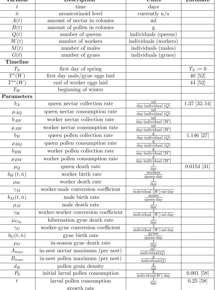
Variable Description Units Estimate
t time days
ˆ
n neonicotinoid level currently n/a A(t) amount of nectar in colonies ml B(t) amount of pollen in colonies g
Q(t) number of queens individuals (queens) W(t) number of workers individuals (workers) M(t) number of males individuals (males)
G(t) number of gynes individuals (gynes)
Timeline
TS first day of spring TS := 0
T∗(W) first day male/gyne eggs laid 40 [52]
T∗∗(W) end of worker eggs laid 44 [52]
TW beginning of winter Parameters
bA queen nectar collection rate day·individual (ml Q) 1.37 [32, 54]
µAQ queen nectar consumption rate day·individual (ml Q) bAW worker nectar collection rate day·individual (ml W) µAW worker nectar consumption rate day·individual (ml W)
bB queen pollen collection rate day·individual (g Q) 1.146 [27] µBQ queen pollen consumption rate day·individual (g Q)
bBW worker pollen collection rate day·individual (g W)
µBW worker pollen consumption rate day·individual (g W)
µQ queen death rate day1 0.0154 [31]
bW(t,n)ˆ worker birth rate queenworkers·day
µW worker death rate day1
γM worker-male conversion coefficient individual (1W)·ml·day
bM(t,n)ˆ male birth rate queenmales·day
µM male death rate day1
γW worker-worker conversion coefficient individual (1W)·ml·day
µGW hibernation gyne death rate
1 day
γG worker-gyne conversion coefficient individual (1W)·ml·day
bG(t,n)ˆ gyne birth rate queengynes·day
µG in-season gyne death rate day1
Amax in-nest nectar maximum (per nest) individual(ml Q)
Bmax in-nest pollen maximum (per nest) individual(g Q)
dB pollen grain density mlg
P0 initial larval pollen consumption individual(g W)·day 0.001 [58] ¯
r larval pollen consumption day1 0.25 [58] growth rate
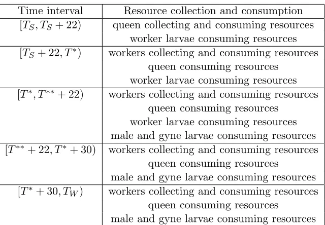
Time interval Resource collection and consumption [TS, TS+ 22) queen collecting and consuming resources
worker larvae consuming resources [TS+ 22, T∗) workers collecting and consuming resources
queen consuming resources worker larvae consuming resources [T∗, T∗∗+ 22) workers collecting and consuming resources
queen consuming resources worker larvae consuming resources male and gyne larvae consuming resources [T∗∗+ 22, T∗+ 30) workers collecting and consuming resources
queen consuming resources
male and gyne larvae consuming resources [T∗+ 30, TW) workers collecting and consuming resources
queen consuming resources
male and gyne larvae consuming resources
Table 2: Seasonal time intervals and corresponding effects of colony members on resources, nectar and pollen.
We now add some assumptions to the model:
• For these preliminary simulations, we simplify the model by letting the worker, male and gyne birth rates bW(t,n), bˆ M(t,n),ˆ and bG(t,n) respectively, be constants.ˆ
• In our model equations for workers, males and gynes, we see the term A(s) +d−B1B(s), quantifying the net resources at time s, which we shall call R(s). Because A is measured in milliliters, and B is measured in grams, it is reasonable to giveRa unit of either ml or g, so without loss of generality, we let Rhave the unit ml. We can convert the mass of pollenB into volume using the density of pollen. In other words,
BV(t) =d−B1B(t),
whereBV(t) denotes the volume of pollen and dB denotes its density (a constant). There are various species
of pollen, each with different specific material densities. According to [15], an estimated value for pollen grain density is 1g/ml. Using this value, we have the following formulation for net resources
R(t) =A(t) +BV(t) =A(t) +d−B1B(t) =A(t) +B(t) =A(t) +B(t),
if we choosedB = 1.
• In the equations for dWdt ,dMdt , and dGdt, we see three parameters γW,γM and γG. As seen in Table 1, these
are conversion coefficients for the production of workers, males, and gynes respectively. In reality, one can think of each as the product of multiple conversion parameters, i.e.,
γk=γkWγkR
for k =W, M, or G, where γkW and γkR have units individual(1 k)·day and 1
ml respectively. It is unreasonable to expect to estimate each of these parameters individually, thus we simply consider each product γk (for
k=W, M, and G).
Caste Total no. incubation days Egg (days) Larva (days) Pupa (days)
Workers 22 4 9 9
Males 26 4 11 11
Gynes 30 4 13 13
Table 3: Bumble bee incubation breakdown by caste
Our model tracks resources (pollen and nectar) and adult colony members (i.e., queens and non-egg,-larval, or -pupal workers, males and gynes). However, because larvae contribute to resource consumption, we must be clear that we are accurately modeling this. In Table 2, we summarize the effects of all colony members on resources (nectar and pollen) at all phases of the season. We tentatively assume, for sake of simplicity, that the last worker emerges when the first male emerges (because of our knowledge of incubation times of 22 and 26 days for workers and males, respectively, and our estimate thatT∗ = 40 andT∗∗= 44, as seen in Table 1). With these assumptions, we have three functions in (3), lW(t, Q), lM(t, Q) and lG(t, Q), which reflect larval pollen consumption, which
require definition.
According to [56, 58, 59] daily pollen intake (measured in mass of pollen per larvae per day) increases exponen-tially as age increases. Therefore, we can model daily pollen intake per worker larvae byP0e¯ra whereameasures age with unit [day], for some positive constantsP0 and ¯r. The number of worker larvae of ageaproduced per day at timetis given by bWQ(t−a), for 4≤a≤13. Therefore, we can model pollen consumption per day by worker
larvae by
lW(t, Q) =
Z 13
4
bWQ(t−a)P0era¯ da. (5)
Similarly, we have
lM(t, Q) =
Z 15
4
bMQ(t−a)P0e¯rada, (6)
for pollen consumption by male larvae and
lG(t, Q) =
Z 17
4
bGQ(t−a)P0era¯ da, (7)
for pollen consumption by gyne larvae. By examining data in [58], we assume that initial larval consumption (per larva)P0is constant across castes, along with exponential consumption rate ¯r. In addition, according to [55], larval diet consists of approximately 34% pollen, and the rest is a combination of nectar and a trivial amount of digestive enzymes. Consequently, we can assume an approximate 2:1 ratio of nectar to pollen for larval consumption, which explains the larval consumption terms in the model for dAdt.
We will refer to the state variables as components of the 6×1-vectorx. As described earlier, delay equations require not only the initial values, η of the states at time 0 (t ≡TS), but also the history information, φ for all
t∈[−r,0), forr defined by the model (in this case,r = 30). For now, we further simplify the model by changing the history information for the gyne population, G. Instead of the exponential decay we see above for t < TS,
we will first assume that G remains non-zero, but some constant value G0, for t < TS. Initially, we made these
choices of history information, letting φbe constant:
η = [A0, B0, Q0,0,0,0]T
whereQ0 =G(TS−1,n) =ˆ G0 (i.e., the number of queens when spring begins is the number of gynes att=−1), and
φ= [0,0,0,0,0, G0]T,
iteratively solving large linear systems, which we shall describe in Section 3). To remediate this, we instead choose a continuous history function by incorporating a “ramp” function for nectar, pollen, queens, and gynes. For example, let φA(t) andηA denote the history function ont ∈[−r,0) for nectar and A(0), respectively. Then we
have
φA(t) =
(
0 −r < t <−2; ηA(−t2+ 1) −2≤t <0;
.
Defining similar ramp functions and incorporating them into our history for pollen, gynes and queens alleviated the computational error faced with the jump discontinuities att= 0.
2.3 Literature search for parameter values
We searched the literature to determine reasonable values for various model parameters. For now, we tentatively fix several parameters at values that produce reasonable colony populations, and aim to estimate these more confidently with experimental data in future work. In Table 1 all model variables, time points, parameters and initial conditions are reported with corresponding units and literature comments. We now comment further on these choices.
In order to quantify queen nectar collectionbAusing ml rather than mg, we used the conversion rate that 1166
mg = 1 ml of 40% sucrose solution, which was used to assimilate nectar in [31, 32].
In order to estimate the queen death rate µQ, we used the information that 14 out of 40 total colonies saw
mother queen loss (hence 26 queens survived) in a given experiment lasting 28 days ( [31]). We performed a simple inverse problem for the model
dQ
dt =−µQQ, Q(0) = 40
with the sole data point Q(28) = 26. This returns the best fitting estimate µQ = 0.0154. The authors of [31]
found that there was no difference in queen loss between control groups and various pesticide treatment groups. Therefore, this should be a reasonable estimate regardless of neonicotinoid exposure.
For the purposes of the first simulation, we use the following information taken from [52] to determine seasonal switch times. Let the term “first egg” denote the first egg laid in the colony, regardless of caste determination. In the experiments conducted in [52], the average time from first egg to last worker emergence was approximately 66 days; assuming a 22 day incubation time, this implies that T∗∗ = 44.The average time from first egg to first emergence of gynes and males was 70 and 65 days respectively. Assuming 30 and 26 day incubation periods for gynes and males, respectively, this provides two estimates forT∗: T∗= 40 orT∗ = 39. Because these values are so similar, we assumeT∗ = 40 for these simulations. Lastly, [52] gives an estimate for the average number of workers produced per day in a given colony, which gives us a direct estimate: bW = 2.4. We initially use this value.
3
Numerical methods
Here we provide a brief summary of the numerical methods used to approximate the solution to (3)-(4), with all further simplifications as detailed in Section 2.2. As mentioned previously, DDEs (sometimes called functional differential equations) differ from ODEs in many ways, including the dimension of the solution. Because (3)-(4) cannot be solved analytically using tools such as the method of steps [11], we must use some type of numerical method to find a finite dimensional approximation to the infinite dimensional solution. Matlab’s built-in DDE solver,dde23, which uses a multi-step method to approximate the solution to a simple DDE with constant delays, is convenient and useful, but limited in scope. One main limitation is the solver’s inability to handle continuum hysteresis terms, which are seen throughout our model, in functions lW, lM, and lG as well as the integral terms
There are many possible choices of solution spaces, one of which is some space of spline functions [2,4,8,40,41]. While the use of cubic and other higher order spline methods can be considered, the authors of [8] found that piecewise linear splines, when implemented with a fairly fine mesh, produced excellent results. Therefore, we explore the use of linear spline functions to approximate the solution to our nonlinear, non-autonomous DDE, the theory of which is partially developed in [4]. In [5], we complete this theory and show that our model satisfies the necessary conditions upon which the theory is based. Here, we summarize this method of approximating the DDE solution.
Consider the following DDE form:
dx
dt =f(t, x(t), xt, x(t−τ1), . . . , x(t−τν)) +g(t), (8) for 0 ≤t ≤ T, x0 =φ , where f =f(η, ψ, y1, . . . , yν) : Z×Rnν → Rn. We define Z = Rn×L2(−r,0;Rn),0 < τ1 < · · · < τν = r, xt(θ) = x(t+θ) for −r ≤ θ ≤ 0 and φ ∈ H1(−r,0). The function g(t) can be understood
as some control function (in the case of our initial model, g(t) ≡ 0). The Banach space L2[a, b] is the space of all continuous, real-valued square integrable functions. The notation Hj or Hj(a, b) denotes the Sobolev space Wj,2(a, b,Rn) of Rn-valued functions f such that f ∈ L2[a, b] and ∂jf ∈L2[a, b]. Specifically, H1 is the space of absolutely continuous functionsf : [a, b]→Rn such that∂f = ˙f ∈L
2[a, b].
In [5], we prove Theorem 1 in [4]; i.e., under certain conditions of f, let y(t;φ, g) = (x(t;φ, g), xt(φ, g)) where
x is the solution of (8) corresponding to φ∈H1, g ∈L2. Then for ζ = (φ(0), φ), y(φ, g) is the unique solution on [0, T] of
z(t) =ζ+ Z t
0
Az(σ) + (g(σ),0)
dσ. (9)
whereA is a nonlinear operator defined in [4]. This equivalent form of the solution to (8) is some function in the infinite-dimensional solution space Z. Therefore, we must choose an appropriate finite dimensional subspace ZN containing the solution approximation. As previously mentioned, our choice for this problem is a space of linear splines. LetPN be the orthogonal projection ofZ onto ZN (see [4] for details). Then, defining the approximating operatorAN =PNAPN, the approximating solution in ZN is defined as
zN(t) =PNζ+ Z t
0
ANzN(σ) +PN(g(σ),0)dσ. (10)
Therefore, we must simply solve this large, but finite-dimensional linear system to approximate the solution to the DDE. As the dimension N of ZN, increases, the solution (10) becomes more accurate, and converges to
the solution of (8). See [5] and [3, 4] for details. BecauseZN is finite dimensional, (10) is equivalent to the ODE system
˙
zN(t) =ANzN(t) +PN(g(t),0), zN(t) =PNζ. (11)
In summary, we have taken an infinite dimensional solution to a DDE and approximated it with a solution to a finite dimensional ODE system. To solve this system over a finite time span, this large matrix system is solved using some method of choice for solving ODEs. In our case, we chose to use Matlab’s stiff ODE solverode15sas it excelled in both accuracy and speed for (3)-(4).
In addition to the linear spline approximation method, we also had to consider how to approximate the numerous integral terms in the model. We chose to use the trapezoidal method, specifically the trapz function given by Matlab. Although the error for this method is higher than that of more refined quadrature methods, this method allowed us to have solutions at all nodal values, without requiring interpolation.
4
Results
With nearly 30 parameters and initial conditions, there are a plethora of combinations we could exhaust in presenting population simulations. Using the fixed values as seen in Table 1, we choose to vary a subset of the remaining unknown parameters and initial conditions to explore a small collection of parameter sets and subsequent population projections. For these simulations we mainly explore worker traits, such as resource collection and consumption and initial worker hatches at timet=TS+ 22 (W0). In one simulation we also vary sexual (male and gyne) birth rates. We choose to present these simulations to demonstrate examples of the changes in population projections due to perturbations in key colony traits. We present four model simulations in Figure 2, each created using parameter sets with slight variations (see Table 4). In all four simulations, we see a slow exponential decay of queen bees and a jump discontinuity in workers, males and gynes at timest=TS+ 22, t=T∗+ 26 andt=T∗+ 30
respectively. Although end-of-season timing depends on weather and geography, we choose TW = TS+ 120 for
these preliminary simulations. We arbitrarily choose Sim 1 as the “baseline” projection seen in Figure 2a, against which we can compare other simulations.
In Sim 2, we change certain worker-related parameters and examine the change in results. As seen in Table 4, we decreased worker nectar and pollen collection, increased worker nectar and pollen consumption, and doubled the initial population of workers, W0. In Figure 2b, we observe very similar dynamics, although higher resource storage is attained. In both simulations, the workers almost die out by winter’s start, and the number of males and gynes surviving by winter’s start are similar.
In Sim 3, we again implement change in worker-related parameters. We decrease worker pollen collection as in Sim 2, and to a lesser degree, decrease worker nectar collection. We again double the initial worker population W0 at time t =TS+ 22, but do not increase worker resource consumption. Comparing Figure 2c to 2a, we see
a much higher nectar storage, and all other dynamics stay quite consistent, including end-of-season worker, male and gyne populations.
Lastly, in Sim 4, we implement all changes seen in Sim 2, but also increase both sexual birth rates, with a substantial increase in the male birth rate bM (see Table 4). Consequently, in Figure 2d, we see similar worker
0 20 40 60 80 100 120 -50
0 50 100 150 200 250
nectar pollen queens workers males gynes
(a) Sim 1
0 20 40 60 80 100 120 -50
0 50 100 150 200 250 300 350
nectar pollen queens workers males gynes
(b) Sim 2
0 20 40 60 80 100 120 -50
0 50 100 150 200 250 300 350 400 450
nectar pollen queens workers males gynes
(c) Sim 3
0 20 40 60 80 100 120 -50
0 50 100 150 200 250 300
nectar pollen queens workers males gynes
(d) Sim 4
Figure 2: Four simulations of bumble bee populations over the interval [TS, TW] using different parameters
Parameter/I.C. Sim 1 Sim 2 Sim 3 Sim 4 bA 1.37 1.37 1.37 1.37
bAW 0.8 0.5 0.6 0.5
µAQ 1 1 1 1
bB 1.146 1.146 1.146 1.146
bBW 0.6 0.4 0.4 0.4
µBQ 0.8 0.8 0.8 0.8
µQ 0.0154 0.0154 0.0154 0.0154
bW 2.4 2.4 2.4 2.4
µW 0.05 0.05 0.05 0.05
γM 5×10⁻⁷ 5×10⁻⁷ 5×10⁻⁷ 5×10⁻⁷
bM 0.7 0.7 0.7 1.2
µM 0.01 0.01 0.01 0.01
γW 5×10⁻⁷ 5×10⁻⁷ 5×10⁻⁷ 5×10⁻⁷
µGW n/a n/a n/a n/a γG 5×10⁻⁷ 5×10⁻⁷ 5×10⁻⁷ 5×10⁻⁷
bG 0.7 0.7 0.7 0.8
µG 0.01 0.01 0.01 0.01
Amax 60 60 60 60
Bmax 60 60 60 60
dB 1 1 1 1
µAW 0.12 0.15 0.12 0.15
µBW 0.12 0.15 0.12 0.15
P0 0.001 0.001 0.001 0.001 ¯
r 0.25 0.25 0.25 0.25
A0 10 10 10 10
B0 10 10 10 10
Q0 20 20 20 20
W0 40 80 80 80
M0 40 40 40 40
G1 40 40 40 40
Table 4: Parameter values and initial conditions (I.C.) used to simulate bumble bee population on the interval [TS, TW]. Any value listed as “n/a” refers to a parameter which is not used in the simulation over the time
period [TS, TW]. Parameters bA, bB, µQ, P0,¯r and bW are fixed at literature values (see Table 1). The remaining
parameters are currently fixed at values that produce reasonable population projections. Q0represents the number of queens at the beginning of the season, which is equivalent to the number of nests. Any circled parameter value represents one that was changed for the purpose of exploring its effect on the ensuing model projections seen in Figure 2.
5
Discussion
in bumble bee reproduction. Although the use of delay terms produced a more complex mathematical problem, we suggested that an ODE model is insufficient to describe bumble bee population dynamics. We presented the population projections in the absence of environmental pressures over one season with four different parameter sets. We saw subsequent changes in the population dynamics, particularly at the beginning of winter.
We chose these four parameter sets to explore life history differences. For instance, Sim 2 represented a decline in worker foraging productivity. This reflected recent studies that have demonstrated that bees exposed to neonicotinoids collected less pollen and returned to the nest less frequently than bees not exposed to neonicotinoids [27, 33, 65], though effects may have varied with particular pesticide configurations [50]. Sim 2 also incorporated greater worker resource consumption, which allowed us to explore different rates of toxin exposure and uptake. Sim 3 explored similar effects without the increase in worker resource consumption. Sim 4 increased sexual birth rates which resulted in a greater male and gyne populations, which in turn will produce more colonies beyond the first season. These simulations hardly exhausted the possible scenarios and outcomes of varying life history traits. However, they provided examples of the ways in which this model can represent bumble bee populations in many environments. In addition, these simulations demonstrated the utility of a DDE model for general population modeling.
Although we have yet to corroborate these simulations with experimental data, the model depicted reasonable seasonal bumble bee dynamics. The authors of [18] also advocated for better understanding of colony growth mechanism in order to more accurately predict queen production and direct efforts to conserve bumblebee popula-tions. In [18], total colony weight was expected to increase exponentially and subsequently decrease once workers begin to die and sexuals begin to leave the nests. As in our model, colony growth was related to resources by modeling colony weight gain as a function of cumulative floral resources. Furthermore, queen production in [18], as in our model, was driven by multiple mechanisms, including floral resources. The authors of [18] found that defining colony growth as a function of floral resources was the best of the models they considered. This supported our proposed model. Lastly, the general trend of increased total population until worker death and sexual dispersal seen in the model and experimental data of [18] lended further support to our proposed model.
As mentioned repeatedly, it is important to understand bumble bee population dynamics in the presence of various environmental pressures, including resource scarcity and insecticide exposure. There are multiple ways to incorporate both lethal and sub-lethal effects of insecticide-exposure, including changes in worker death rate, worker collection rate, worker productivity rates, queen death rate, and queen reproduction rates. One can also define the above parameters as functions of insecticide exposure, rather than as constants. In addition, one can implement changes due to environmental effects by exploring variable reproductive switch times, maximum resource availability, etc. By comparing model results to experimental data in the absence and presence of these pressures, one can test the model’s accuracy. Lastly, the linear spline approximation method, with a mesh size of 1/8, was both accurate and efficient. We took advantage of Matlab’s excellent ODE solvers to solve the approximating ODE system (11). With the model and techniques and outlined here, it is also feasible to approximate multi-year projections.
6
Conclusion
7
Acknowledgements
We thank Oliver Schweiger for assisting with parameter values collected from the literature. This research was supported by the Air Force Office of Scientific Research under grant numbers AFOSR FA9550-12-1-0188 and AFOSR FA9550-15-1-0298, by a CRSC/Lord Fellowship, by the August T Larson guest researchers programme at the Swedish University of Agricultural Sciences, and by the Swedish research council FORMAS.
References
[1] Boris Baer and Paul Schmid-Hempel, Sperm influences female hibernation success and fitness in the bumble beeBombus terrestris,Proc. Biol. Sci 272:1560 (2005), 319–23.
[2] H.T. Banks, Delay systems in biological models: approximation techniques,Nonlinear Systems and Applica-tions(V. Lakshmikantham, ed.), Academic Press, New York (1977) 21–38.
[3] H.T. Banks, Approximation of nonlinear functional differential equation control systems, J. Optim. Theor. Applic.,24 (1979) 383–408.
[4] H.T. Banks, Identification of nonlinear delay systems using spline methods, in Proc. Int. Conf. Nonlinear Phenomena in Math. Sci., Arlington, Texas, Academic Press, New York (1982).
[5] H.T. Banks, J.E. Banks, R. Bommarco, M. Rundl¨of, and K. Tillman, Analysis of nonlinear delay systems with applications in bumble bee population models, CRSC-TR16-xx, N.C. State University, Raleigh, NC, June, 2016, to appear.
[6] H.T. Banks and J.A. Burns, Hereditary control problems: numerical methods based on averaging approxi-mations,SIAM J. on Control and Optim.16 (1978) 169–208.
[7] H.T. Banks, S. Hu, and W.C. Thompson, Modeling and Inverse Problems in the Presence of Uncertainty, CRC Press, New York (2014).
[8] H.T. Banks and F. Kappel, Spline approximations for functional differential equationsJ. Diff. Eq.34(1979), 496–522.
[9] H.T. Banks and H.T. Tran, Mathematical and Experimental Modeling of Physical and Biological Processes, CRC Press, Boca Raton, FL (2009).
[10] I. Bartomeus, et. al., Historical changes in northeastern US bee pollinators related to shared ecological traits.
Proc. Natl Acad. Sci. USA110, (2013) 4656–4660.
[11] A. Bellen and M. Zennaro, Numerical Methods for Delay Differential Equations, Oxford, New York (2003).
[12] Ted Benton,Bumble bees, HarperCollins, London (2006).
[13] J.C. Biesmeijer, et. al., Parallel declines in pollinators and insect-pollinated plants in Britain and the Nether-lands.Science313, (2006) 351–354.
[14] R. Bommarco, O. Lundin, H.G. Smith, and M. Rundl¨of, Drastic historic shifts in bumble-bee community composition in Sweden.Proc. R. Soc. B 279, (2012) 309–315.
[15] James S. Borrell, Rapid assessment protocol for pollen settling velocity: implications for habitat fragmenta-tion,Bioscience Horizons 5(2012), hzs002.
[17] C. Carvell, A.F. Bourke, J.L. Osborne, and M.S. Heard, Effects of an agri-environment scheme on bumblebee reproduction at local and landscape scales,Basic Appl. Ecol.,16, (2015) 519–530.
[18] Elizabeth E. Crone and Neal M. Williams, Bumble bee colony dynamics: quantifying the importance of land use and floral resources for colony growth and queen production,Ecology Letters,19, (2016) 460–468.
[19] D.T. Crouse, L.B. Crowder and H. Caswell, A stage-based population model for loggerhead sea turtles and implications for conservation,Ecology 68, (1987) 1412–1423.
[20] J. M. Cushing, Integrodifferential Equations and Delay Models in Population Dynamics, Lec. Notes in Biomath.,20, Springer-Verlag, NY (1977).
[21] J.M. Duchateau, Agonistic behaviors in colonies of the bumble bee Bombus terrestris, J. Ethol. 7 (1989), 141–152.
[22] M.J. Duchateau and H.H.W. Velthuis, Development and Reproductive Strategies in Bombus terrestris
Colonies,Behaviour 107:3, (1988) 186-207.
[23] M.J. Duchateau, H.H.W. Velthius, and J.J. Boomsma, Sex ratio variation in the bumble beeBombus terrestris,
Behav. Ecol.15:1, (2004) 71-82.
[24] Y.L. Dupont, C. Damgaard, and V. Simonsen, Quantitative historical change in bumble bee (Bombus spp.) assemblages of red clover fields. PLoS ONE6, (2011) e25172.
[25] A. Elbert, M. Haas, B. Springer, W. Thielert, and R. Nauen, Applied aspects of neonicotinoid uses in crop protection.Pest Manag. Sci. 64, (2008) 1099–1105.
[26] Aline Fauser-Misslin, Ben M. Sadd, Peter Neumann, and Christoph Sandrock, Influence of combined pesticide and parasite expose on bumble bee colony traits in the laboratory,Journal of Applied Ecology51(2014), 450– 459.
[27] Hannah Feltham, Kirsty Park, and Dave Goulson, Field realistic doses of pesticide imidacloprid reduce bumble bee pollen foraging efficiency,Ecotoxicology3 (2014): 317–23.
[28] C. Fontaine, I. Dajoz, J. Meriguet. and M. Loreau, Functional diversity of plant-pollinator interaction webs enhances the persistence of plant communities.PLoS Biology,4:1, (2006) e1.
[29] L.A. Garibaldi, et. al., Wild pollinators enhance fruit set of crops regardless of honey-bee abundance,Science
339(6127), (2103) 1608–1611.
[30] Guedes, R. N. C., Smagghe, G., Stark, J. D., & Desneux, N. (2016). Pesticide-Induced Stress in Arthropod Pests for Optimized Integrated Pest Management Programs.Annual Review of Entomology0, (2016).
[31] Richard J. Gill, Oscar Ramos Rodriguez and Nigel E. Raine, Combined pesticide exposure severely affects and individual- and colony-level traits in bees,Nature 491, (2012) 105–08.
[32] Richard J. Gill, Oscar Ramos Rodriguez and Nigel E. Raine, Combined pesticide exposure severely affects and individual- and colony-level traits in bees: Supplementary Material,Nature 491, (2012).
[33] R. J. Gill and N.E. Raine, Chronic impairment of bumblebee natural foraging behaviour induced by sublethal pesticide exposure.Functional Ecology28, (2014) 1459–71.
[34] H.C.J. Godfray et. al., A restatement of the recent advances in the natural science evidence base concerning neonicotinoid insecticides and insect pollinators. Proc. Biol. Sci.282, (2015).
[36] Goulson, D.,Bumble bees, 2nd ed., Oxford, Oxford, U.K., (2010).
[37] Goulson, D., Review: An overview of the environmental risks posed by neonicotinoid insecticides.J. of Applied Ecology,50(4) (2013) 977–987.
[38] Jacob G. Holland, Florian S. Guidat, and Andrew F.G. Bourke, Queen control of a key life-history even tin a eusocial insect,Biology Letters,9: 20130036, (2013).
[39] G.E. Hutchinson, Circular causal systems in ecology, Ann. N.Y. Acad. Sci.,50, (1948) 221–246.
[40] F. Kappel and W. Schappacher, Autonomous nonlinear functional differential equations and averaging ap-proximations, Nonlinear Analysis2, (1978) 391-422.
[41] F. Kappel, Spline approximations for autonomous nonlinear functional differential equations, Nonlinear Anal-ysis, Theory, Methods and App.10:5 (1986), 503-513.
[42] David S. Khoury, Andrew B. Barron, and Mary R. Myerscough, Modelling food and population dynamics in honey bee colonies,PLoS ONE 8(5): e59084 (2013). doi:10.1371/journal.pone.0059084
[43] D. Kleijn et. al., Delivery of crop pollination services is an insufficient argument for wild pollinator conserva-tion.Nature Communications6, (2015).
[44] A.M. Klein, B.E. Vaissi`ere. J.H. Cane, I. Steffan-Dewenter, S.A. Cunningham, C. Kremen, and T. Tscharntke, Importance of pollinators in changing landscapes for world crops.Proceedings of the Royal Society of London Series B: Biological Sciences274 (2007), 303–313.
[45] M. KotElements of Mathematical Ecology, Cambridge University Press, Cambridge, U.K., (2001).
[46] C. Lopez-Vaamonde, et. al., Lifetime reproductive success and longevity of queens in an annual social insect,
J. Evol. Biol.22:5, (2009) 983–96.
[47] O. Lundin, M. Rundl¨of, H.G. Smith, I Fries, and R. Bommarco, Neonicotinoid insecticides and their impacts on bees: a systematic review of research approaches and identification of knowledge gaps, PLoS ONE 10:8, (2015) e0136928.
[48] S. Macfadyen, J.E. Banks, J.D. Stark, and A.P. Davies, Using semifield studies to examine the effects of pesticides on mobile terrestrial invertebrates, Annual Review of Entomology,59:1 (2014) 383.
[49] Malone et. al., Effects of four protease inhibitors on the survival of worker bumble bees, Bombus terrestris.
Apidologie31, (2000) 25–38.
[50] C. Moffat, S.T. Buckland, A. J. Samson, et. al., Neonicotinoids target distinct nicotinic acetylcholine receptors and neurons, leading to differential risks to bumblebees.Scientific Reports 6: 24764 (2016).
[51] W.F. Morris, and D.F. Doak, Quantitative conservation biology: Theory and practice of population viability analysis. Sinauer Associates, Sunderland, MA, USA, (2002).
[52] Christine B. M¨uller, Jacqui A. Shykoff, and Gillian H. Sutcliffe, Life history patterns and opportunities for queen-worker conflict in bumble bees,Oikos, Copenhagen65(1992), 242–48.
[53] J. Ollerton, R. Winfree, and S. Tarrant, How many flowering plants are pollinated by animals?,Oikos120(3), (2011) 321–26.
[54] James Peat and Dave Goulson, Effects of experience and weather on foraging rate and pollen versus nectar collection in the bumble bee,Bombus terrestris,Behav. Eco. Sociobiol.58(2005), 152–56.
[56] J.J.M. Pereboom, H.H.W. Velthuis, and M.J. Duchateau, The organization of larval feeding in bumble bees (Hymenoptera, Apidea) and its significance to caste differentiation,Insectes Soc50 (2003), 127–133.
[57] S.G. Potts, J.C. Biesmeijer, C. Kremen, P. Neumann, O. Schweiger, and W.E. Kunin, Global pollinator declines: trends, impacts and drivers,Trends Ecol. Evol.25, (2010) 345–354.
[58] M.F. Ribeiro, Growth in bumble bee larvae: relation between development time, max and amount of pollen digested,Canadian J. of Zoology 72:11 (1994), 1978–1985.
[59] M.F. Ribeiro, H.H.W. Velthuis, M.J. Duchateau, and I. van der Tweel, Feeding frequency and caste differen-tiation inBombus terrestris larvae, Insectes Soc.46(1999), 306–314.
[60] R¨oselber, P.F. Unterschiede in der Kastendetermination zwischen den hummelk¨oniginnen (Hym., Apoidea, Bombinae),Adipologie 4 (1970), 267–274.
[61] M. Rundl¨of, A.S. Persson, H.G. Smith, and R. Bommarco, Late-season mass-flowering red clover increases bumble bee queen and male densities.Biol. Conserv.,172, (2014) 138–145.
[62] M. Rundl¨of, G.K.S. Andersson, R. Bommarco, I. Fries, V. Hederstr¨om, L. Herbertsson, O. Jonsson, B.K. Klatt, T.R. Pedersen, and J. Yourstone, and H.G. Smith, Seed coating with a neonicotinoid insecticide negatively affects wild bees.Nature 521, (2015) 77–80.
[63] P. Smeets, and M. Duchateau, Longevity ofBombus terrestrisworkers (Hymenoptera: Apidae) in relation to pollen availability, in the absence of foraging.Apidologie,34:4, (2003) 333–337.
[64] Hal Smith, An Introduction to Delay Differential Equations with Applications to the Life Sciences, Springer, NY, (2011).
[65] D.A. Stanley, P.D. Garratt, J.B. Wickens, et. al., Neonicotinoid pesticide exposure impair crop pollination services provided by bumblebees.Nature 528(7583), (2015) 548-550.
[66] J.D. Stark, and J.E. Banks, “Selective pesticides”: are they less hazardous to the environment?, Bioscience
51, (2001) 980–982.
[67] G.H. Sutcliffe and R.C. Plowright, The effects of pollen availability on development time in the bumble bee
Bombus terricola (Hymenoptera, Apidae),Canadian J. Zoology 68, (1990) 1120–23. doi: 10.1139/z90-166.
[68] H.H.W. Velthius, Development and reproductive strategies in Bombus terrestris colonies, Behaviour 107, (1988) 186–207.
[69] P.R. Whitehorn, S. O’Connor, S., F.L. Wackers, and D. Goulson, Neonicotinoid pesticide reduces bumble bee colony growth and queen production.Science336, (2012) 351–352.
[70] N.M. Williams, J. Regetz, and C. Kremen, Landscape-scale resources promote colony growth but not repro-ductive performance of bumble bees, Ecology93, (2011) 1049–1058.
[71] R. Winfree, I. Bartomeus and D.P. Cariveau, Native pollinators in anthropogenic habitats.Annu. Rev. Ecol. Evol. Syst.,42, (2011) 1–22.


![Figure 2: Four simulations of bumble bee populations over the interval [TS, TW ] using different parameters pre-sented in Table 4.](https://thumb-us.123doks.com/thumbv2/123dok_us/1581890.1194804/12.612.65.556.60.489/figure-simulations-bumble-populations-interval-dierent-parameters-sented.webp)
![Table 4: Parameter values and initial conditions (I.C.) used to simulate bumble bee population on the interval[TS, TW ].Any value listed as “n/a” refers to a parameter which is not used in the simulation over the timeperiod [TS, TW ]](https://thumb-us.123doks.com/thumbv2/123dok_us/1581890.1194804/13.612.158.457.50.549/parameter-conditions-simulate-population-interval-parameter-simulation-timeperiod.webp)