©
DOI: 10.1534/genetics.104.036236
Bayesian Analysis of an Admixture Model With Mutations
and Arbitrarily Linked Markers
Laurent Excoffier,*
,†,1Arnaud Estoup* and Jean-Marie Cornuet*
*Institut National de la Recherche Agronomique, Centre de Biologie et de Gestion des Populations (CBGP), Campus International de Baillarguet, 34988 Montferrier-sur-Lez Cedex, France and†Computational and Molecular Population
Genetics Lab (CMPG), Zoological Institute, University of Bern, 3012 Bern, Switzerland Manuscript received September 13, 2004
Accepted for publication December 1, 2004
ABSTRACT
We introduce here a Bayesian analysis of a classical admixture model in which all parameters are simultaneously estimated. Our approach follows the approximate Bayesian computation (ABC) framework, relying on massive simulations and a rejection-regression algorithm. Although computationally intensive, this approach can easily deal with complex mutation models and partially linked loci, and it can be thoroughly validated without much additional computation cost. Compared to a recent maximum-likeli-hood (ML) method, the ABC approach leads to similarly accurate estimates of admixture proportions in the case of recent admixture events, but it is found superior when the admixture is more ancient. All other parameters of the admixture model such as the divergence time between parental populations, the admixture time, and the population sizes are also well estimated, unlike the ML method. The use of partially linked markers does not introduce any particular bias in the estimation of admixture, but ML confidence intervals are found too narrow if linkage is not specifically accounted for. The application of our method to an artificially admixed domestic bee population from northwest Italy suggests that the admixture occurred in the last 10–40 generations and that the parental Apis melliferaand A. ligustica populations were completely separated since the last glacial maximum.
H
YBRID populations have been central to theories likelihood-based methods, including Bayesian (Chikhion adaptation and speciation (Barton 2001), et al.2001) and maximum-likelihood (Wang2003) ap-and their study has encountered a new interest since it proaches, are computationally intensive but have been was shown that they could be ideal in detecting disease shown to produce estimates with smaller variances genes (ChakrabortyandWeiss1988). The assessment across independent replicates or simulations, especially of the degree of admixture of a given population has when the estimate was based on a small number of loci traditionally relied on the comparison of allele frequen- (Wang2003;Choisyet al.2004). A promising alterna-cies between two potential parental populations and a tive to these methods has been the development of an putative hybrid population (RobertsandHiorns1965; approach using nongenetic information to more
pre-ChakrabortyandWeiss1988;Long1991). Recently, cisely define the contribution of sampled populations these methods have been improved by incorporating to the hybrid (Gaggiotti et al. 2002, 2004). Finally, information on the molecular diversity present in the recognizing that a major drawback of all these former admixed and in parental populations (Bertorelleand approaches is to require an explicit definition of the
Excoffier 1998; Dupanloup and Bertorelle 2001) source populations, some recent methods have at-or by explicitly taking into account the genetic drift of tempted to identify admixed individuals without requir-allele frequencies since the admixture event (Chikhiet ing the source parental populations to be defined al. 2001; Wang 2003). However, the accuracy of the (Pritchard et al. 2000; Dawson and Belkhir 2001; estimation of the contribution of the parental popula- Anderson and Thompson 2002; Falushet al. 2003), tions to the hybrid depends highly on the extent of but their statistical power remains to be assessed. differentiation between parental populations (Bertor- As stated previously, a common problem with most elleandExcoffier1998) and the time elapsed since of the previous methods is their inability to explicitly the admixture event (Chikhi et al.2001;Choisyet al. handle mutations (but seeBertorelleandExcoffier
2004). No single method was found to date superior to 1998;Dupanloupet al.2004), whereas this is likely to others in all circumstances (Choisyet al.2004). Recent be particularly important when the admixture event is
ancient. While ML methods have the potential to pro-vide accurate estimations of demographic and muta-1Corresponding author:Computational and Molecular Population
Ge-tional parameters, the calculation of likelihoods under
netics Lab, Zoological Institute, University of Bern, Baltzerstrasse 6,
3012 Bern, Switzerland. E-mail: [email protected] models of nonrecent hybridization events for which
tations have to be taken into account at both indepen-dent and partially linked markers remains problematic. A powerful Bayesian alternative to likelihood computa-tion for parameter estimacomputa-tion has been introduced re-cently (FuandLi1997;Tavare´et al.1997;Pritchard et al.1999;Estoupet al.2001), dubbed as approximate Bayesian computation (ABC; Beaumont et al. 2002;
Marjoramet al.2003). This approach does not require the computation of likelihoods, but simply relies on the comparison of summary statistics computed on ob-served data with those computed on data simulated under a model for which the parameters of interest are known (Beaumontet al.2002;Marjoramet al.2003). Although the ABC method relies on summary statistics and thus does not use all available data, it has been shown to provide very accurate results in the analysis of relatively simple evolutionary scenarios where full maximum-likelihood methods were available ( Beau-mont et al. 2002; Marjoram et al. 2003). Hence, by construction, ABC methods have the potential to con-sider models of any complexity, provided only that data
Figure 1.—Admixture model considered in this study. A
can be simulated under the model. Recent applications hybrid population is createdtADMgenerations ago from a mix-of the latest developments mix-of ABC methods (Beaumont ture of two parental populations that divergedtDIVgenerations before admixture time. Except for the admixture event itself,
et al.2002) illustrate their potential for the analysis of
all populations are genetically isolated. The demographic
complex demographic scenarios (Estoup and Clegg
model is characterized by seven parameters, which are the
2003;Estoupet al.2004). Recent coalescent-based pack- effective number of genes in the ancestral (N0), parental (N1 ages (e.g.,Hudson2002;LavalandExcoffier2004) andN2), and admixed (NA) populations; the times of admix-provide an efficient tool for simulating genetic data ture (tADM) and divergence (tDIV); as well as the admixture proportion () taken as the relative contribution of parental
under complex scenarios (including introgression or
population 1 to the admixed population.
hybridization scenarios) and have the potential to gen-erate data for independent or partially linked markers. Such versatile simulation packages make it possible,
in Figure 1 and similar to that used in previous studies even for biologists unfamiliar with simulation
algo-(e.g., Long 1991; Bertorelle and Excoffier 1998; rithms, to perform parameter estimation under the ABC
Wang2003;Choisyet al.2004). framework and consider various evolutionary scenarios.
The genetic model:Unlike almost all methods consid-In this article, we apply the ABC method to the
estima-ering that gene frequencies evolve only through genetic tion of all the parameters of an explicit admixture model
drift, our approach also takes mutations into account (Figure 1) defined previously (Bertorelleand
Excof-(as inBertorelleandExcoffier1998). This involves
fier1998;Wang2003) and described inmethods. We
the choice of a mutation model and of its parameters. use the SIMCOAL2 coalescent simulation program
We restricted our study to microsatellite markers for (LavalandExcoffier2004) to generate a large
num-which we used a multistep mutation model, sometimes ber of microsatellite data sets for random values of the
called generalized stepwise mutation (GSM) model (
Zhi-admixture model parameters, on which several
sum-votovskyet al.1997;Estoupet al.2002), requiring two mary statistics are evaluated. These simulated summary
parameters per locus: the mutation rate (i) and the statistics are used for parameter estimation in a series
coefficient (Pi) of the geometric distribution of the of test data sets, which allows us to validate our approach
length by which a new mutant allele differs from its and to compare its performance with a previously
pub-ancestor. However, these two series of parameters are lished maximum-likelihood (ML) method (Wang2003).
considered as nuisance parameters, and we will pay at-The method is then applied to the case of an admixed
tention only to their average values across loci:andP. population of honeybees from northwestern Italy.
Data thus consist here of multilocus genotypes of n
individuals sampled from each of the three populations.
The ABC approach: The rationale and the full
de-METHODS
scription of the ABC method are given inBeaumont et al.(2002). In short, the approach involves three
suc-The demographic model:To compare the behavior
statistics, retaining the simulations that are arbitrarily close to the observations, and rejecting the other simula-tions. Finally, the third step is the estimation of the parameters by performing a multiple and locally weighted linear regression on the summary statistics associated with the retained simulations. The set of sim-ulations retained for parameter estimation was selected by strictly followingBeaumontet al.(2002), by comput-ing a Euclidean distance (␦) between simulated and observed summary statistics and retaining the 1000 sim-ulations having the smallest␦ distance (being closest) to the test data set.
The SIMCOAL2 program (Laval and Excoffier
2004), freely available on http://cmpg.unibe.ch/soft ware/simcoal2, has been used to generate microsatellite data sets in the first step, and a new program (abcEst) has been developed for parameter estimation (step 3 in Figure 2). The program abcEst (Windows or Linux version) is available from L. Excoffier upon request. Compared to the published version of the SIMCOAL2 program, two enhancements were added: the imple-mentation of the generalized stepwise mutation model and the possibility of having different mutation rates at different loci. Microsatellite allele size constraints were included in our simulations by imposing reflecting boundaries at the edge of an allele size range of 30 continuous allelic states (Feldmanet al.1997;Pollock et al.1998). This range is consistent with empirical data on repeat numbers at microsatellites in various species (e.g.,Garzaet al.1995;GoldsteinandPollock1997;
Estoupet al.2000).
Regarding mutation modeling, we draw for each sim-ulation an average mutation rate across loci from a log Uniform distribution, and individual locus mutation rates are then drawn from a Gamma distribution with mean equal to. A similar procedure is also used for the average and individual locus coefficients of the geo-metric distribution of step lengthsPandPi(see Table 1 for details). Note that we have chosen to implement this hierarchy of parameters and did not draw
locus-Figure2.—Synopsis of the ABC parameter estimation ap- specific parametersiandPifrom unique distributions,
proach. Step 1 usually includes a loop over hundreds of thou- since the average parametersandPwould have been sands to millions of simulations. It is the most time-consuming virtually identical across simulations of a large number task, generally involving several days of computations. In
con-of loci and equal to the mean con-of the priors. Their
estima-trast, the computations in steps 2 and 3 usually take seconds
tion would thus have been meaningless. Note also that
or minutes. To validate the ABC approach, steps 2 and 3
can be repeated hundreds of times on pseudo-observed data we have chosen a relatively broad prior forcompared
generated by step 1-type simulations based on fixed prede- to previous studies (e.g., Wilsonand Balding1998),
fined parameter values. such as to cover a wide range of possible mutation rates
(see Table 1).
In addition to the 9 basic parameters of the admixture model (the admixture proportion, the four effective lion) multilocus data sets with characteristics similar to
the observed data set (same number of samples, same population sizes, the time of divergence tDIV, the time
of admixturetADMcounted in generations, and the
muta-number of individuals per sample, same muta-number of
loci), using parameter values randomly drawn from tional parametersandP), 11 composite parameters were computed and recorded. They correspond, respec-some prior distributions (as defined in Table 1). The
second step consists of comparing the simulated data set tively, to the times of divergence and admixture scaled by the population sizes (t/Ni, witht ⫽tADMortDIV, and
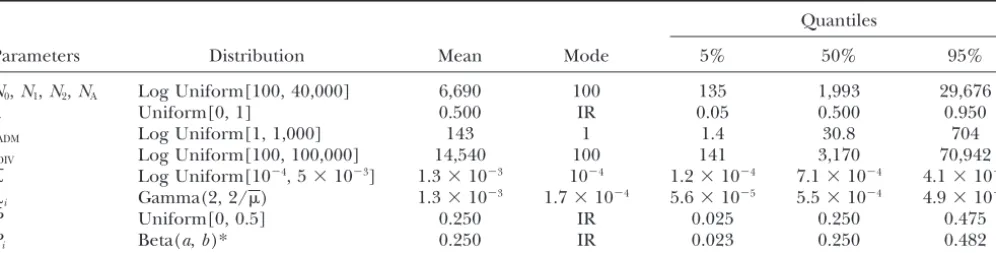
TABLE 1
Prior distributions of simulated parameters
Quantiles
Parameters Distribution Mean Mode 5% 50% 95%
N0,N1,N2,NA Log Uniform[100, 40,000] 6,690 100 135 1,993 29,676
Uniform[0, 1] 0.500 IR 0.05 0.500 0.950
tADM Log Uniform[1, 1,000] 143 1 1.4 30.8 704
tDIV Log Uniform[100, 100,000] 14,540 100 141 3,170 70,942
Log Uniform[10⫺4, 5⫻10⫺3] 1.3⫻10⫺3 10⫺4 1.2⫻10⫺4 7.1⫻10⫺4 4.1⫻10⫺3
i Gamma(2, 2/) 1.3⫻10⫺3 1.7⫻10⫺4 5.6⫻10⫺5 5.5⫻10⫺4 4.9⫻10⫺3
P Uniform[0, 0.5] 0.250 IR 0.025 0.250 0.475
Pi Beta(a,b)* 0.250 IR 0.023 0.250 0.482
N0,N1,N2, andNA, effective population size (number of gene copies) in ancestral (N0), parental (N1andN2), and admixed (NA) populations, respectively;, contribution of parental population 1 to the admixed population;tADM, time since admixture; tDIV, divergence time between parental populations before admixture; and i, average and individual-locus mutation rates,
respectively;Pand Pi, average and individual-locus parameters of the geometric distribution of the GSM, respectively; *Prior
distribution forPiis as follows: ifPⱖ0.001 then P⫽Beta(a, b) witha⫽0.5⫹199Pandb⫽a(1⫺P)/P; otherwiseP⫽0.
IR, irrelevant.
i⫽0, 1, 2, orA), to the population sizes scaled by the pect heterozygosity to be informative for the estimation of population size, but it should also depend on the mutation rate (i⫽2Ni, withi⫽0, 1, 2, andA), and
to the times of divergence and admixture scaled by admixture proportion in the hybrid population. Also, pairwiseFST’s are expected to bring information about
the mutation rate ( ⫽ 2t, witht⫽ tADMor tDIV). The
estimation procedure was thus carried out separately divergence times between parental populations and about admixture proportions. ThemYadmixture coeffi-on the 9 basic parameters as well as coeffi-on the 11 composite
parameters. cient should obviously bring information on admixture
proportion, whileD⬘in the admixed population should
Summary statistics:The following 15 summary
statis-tics were computed on all the simulated microsatellite decay with admixture time, but also depend on the absolute sizes of the populations (drift). However, we data sets: the average number of alleles over loci for
each of the two parental and the admixed population did not attempt here to define an optimal set of statistics or to study the effect of removing or adding summary samples, the average heterozygosity over loci and
aver-age modifiedMstatistics (GarzaandWilliamson2001) statistics, which could be the subject of a later study.
Simulated data sets:A first series of 106data sets was
over loci for the same three samples, the (␦)2genetic
distance (Goldsteinet al.1995) between the two paren- simulated and consisted of 50 diploid individuals (100 genes) typed at 50 independent microsatellite loci. This tal population samples, the measure of differentiation
FST(WeirandCockerham1984) between all three pairs large data set was fractioned into subsets to study the
effect of sample size and number of loci on parameter of population samples, the average extent of linkage
disequilibriumD⬘between independent markers in the estimation, and thus data sets consisting of 5, 10, 20, and 50 loci studied in samples of 20 and 100 genes were admixed population, and themYadmixture coefficient
estimator (BertorelleandExcoffier1998). The for- obtained. A second series of 106data sets, consisting of
50 diploid individuals typed at a mixture of 20 indepen-mula of the modified M statistics is 兺L
l⫽1kl/兺Ll⫽1(1⫹rl),
where klis the number of alleles at the lth locus,rl is dent and partially linked loci, was simulated. The 20 loci consisted of two unlinked groups of 10 partially the difference in number of repeats between the largest
and the smallest allele at locusl(i.e., the range of allele linked loci. Each group of 10 partially linked loci was itself divided into two subsets of 5 completely linked sizes), and L is the number of loci. Compared to its
original definition (Garza and Williamson 2001), it loci (genetic distance of 0 cM), 1 cM distant from each other. The 190 pairs of loci thus fell into three linkage just avoids a division by zero when a gene sample is
fixed for a single allele. Note that the summary statistics categories: unlinked (100 pairs of loci), partially linked at 1 cM (50), and totally linked (40). The coefficient were chosen such as to capture different features of the
data, both at the within- and at the between-population of linkage disequilibrium D⬘ was computed separately in the three categories of markers, thus adding two level. This choice is partially arbitrary, since there is
currently no objective way to define an optimal set of summary statistics to these simulated data sets with re-combination. Note that our choice of three categories statistics (Beaumontet al.2002), but we have tried to
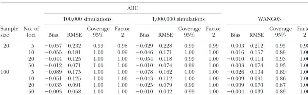
ex-TABLE 2
Effect of the number of independent loci on the estimation of the admixture rateby the ABC andWang’s (2003) methods
ABC
100,000 simulations 1,000,000 simulations WANG03
Sample No. of Coverage Factor Coverage Factor Coverage Factor
size loci Bias RMSE 95% 2 Bias RMSE 95% 2 Bias RMSE 95% 2
20 5 ⫺0.057 0.232 0.99 0.98 ⫺0.029 0.228 0.99 0.99 0.003 0.212 0.95 0.98
10 ⫺0.055 0.181 1.00 0.99 ⫺0.046 0.171 1.00 1.00 0.016 0.157 0.89 1.00
20 ⫺0.044 0.125 1.00 1.00 ⫺0.054 0.118 0.99 1.00 ⫺0.010 0.114 0.93 1.00
50 ⫺0.012 0.071 1.00 1.00 ⫺0.010 0.074 0.99 1.00 0.003 0.074 0.93 1.00
100 5 ⫺0.089 0.175 1.00 1.00 ⫺0.078 0.162 1.00 1.00 ⫺0.026 0.134 0.89 1.00
10 ⫺0.051 0.125 1.00 1.00 ⫺0.043 0.112 1.00 1.00 ⫺0.009 0.091 0.86 1.00
20 ⫺0.035 0.091 1.00 1.00 ⫺0.025 0.079 0.99 1.00 ⫺0.009 0.070 0.87 1.00
50 ⫺0.003 0.058 1.00 1.00 ⫺0.010 0.042 0.99 1.00 ⫺0.004 0.039 0.89 1.00
Simulated conditions are independent loci. ⫽0.3,tADM⫽5, tDIV⫽5000,N0⫽N1⫽N2⫽300. Bias and root mean square error (RMSE) are expressed in relative units. Coverage 95% represents the number of times among 100 that the true value of
(0.3) lies within the estimated 95% confidence interval. Factor 2 represents the number of times that the true value oflies within an interval limited by 50 and 200% of the estimatedvalue.
justify and are commonly found in many data sets, the evaluation was thus performed in seven situations. Due to the huge amount of computations needed for the spacing of 1 cM was chosen such as to have a different
amount of loss of potential disequilibrium created by comparisons presented here, a few parameters were fixed across the simulations. The population sizes (num-the admixture process over (num-the time periods studied
below. Indeed, one would expect that markers 1 cM bers of genes) were set to 300, the average mutation rate to 0.0005 (reviewed in Ellegren2004), and the apart would loseⵑ5, 63.4, and 98.2% of the original
disequilibrium caused by the admixture after 5, 100, geometric coefficientsPto 0.3 (e.g.,Estoupet al.2002). The first situation modeled a recent admixture (tADM⫽
and 400 generations, respectively, thus allowing one to
potentially use linkage disequilibrium (LD) to estimate 5 generations,i.e.,tADM/Ne⫽0.0167), an ancient
diver-gence (tDIV⫽5000 generations,i.e.,tDIV/Ni⫽16.7), and admixture time.
Performance evaluation and test data sets: The per- an admixture proportion of 0.3. This situation was used to evaluate the effects of different numbers of loci and of formances of our ABC approach were evaluated in a
series of samples having fixed values of the admixture different sample sizes (Table 2). The other six situations were chosen to evaluate the effects of increasing the model. For each combination of parameters, the
SIM-COAL2 program was used to generate 100 data sets, on time of admixture for two different admixture propor-tions and of having partially linked markers. The perfor-which summary statistics were computed and then used
as pseudo-observed summary statistics. The same data mance of our ABC method and of WANG03 was charac-terized by therelative bias(average difference between set was also used as input to a recent ML method (Wang
2003) denoted hereafter WANG03. The latter method the estimate and the true value divided by the true value), therelative root mean square error(RMSE—square has been chosen for a comparison with our approach,
because it has been shown to produce good estimates root of the mean square error divided by the true value), the 95% coverage (proportion of times in which the of admixture coefficients, and because it estimates other
parameters of the admixture model that can be also true value is within the equal-tailed 95% confidence or credible interval around the estimate), and thefactor 2
compared with those of our ABC method. Moreover,
compared to the method ofChikhiet al.(2001), Wang’s (proportion of times in which the estimated value is in an interval bounded by values equal to 50 and 200% ML method was notably faster, allowing us to get 100
estimates for fixed simulated parameter values in a rea- that of the true value). All measurements of bias, RMSE, and factor 2 were computed by taking the mode of the sonable amount of time.
It is worth noting that while the simulation of 1 million posterior distribution as a point estimate. The factor 2 parameter is intuitively appealing and brings qualita-data sets and the computation of their associated
sum-mary statistics for our ABC approach is time consuming tively different information than the 95% coverage. It indeed tells users how often the estimator is arbitrarily (ⵑ12 hr on 15 computer nodes), the ABC estimation
of the parameters on a given test data set takes only close (factor 2 here) to the true value, while the inclu-sion of the true value within a confidence interval does seconds to minutes, so that the evaluation of the
Figure 3.—Posterior distributions of some parameters of the admixture model. We contrast here posterior distributions obtained from an analysis performed on a set of 1 million (solid line) or 100,000 (dashed line) simulated summary statistics. In both cases, the estimation and the posterior distribution were obtained by a local weighted regression (Beaumontet al.2002) on the 1000 simulations closest to the test data set. True parameter values are shown as vertical boldface lines:N⫽300 for all population sizes; admixture rate, ⫽0.3; divergence time between populations,tDIV⫽5000 generations; admixture time,tADM⫽ 5; mutation rate, ⫽5⫻10⫺4; and parameter of the geometric distribution of mutation steps,P⫽0.3. Note that the posterior distributions shown here are the output of a single (randomly chosen) analysis, and that they are not averaged over 100 replicates as reported in Tables 2–4.
All measures of performance were estimated over 100 analysis of a single (randomly chosen) case from 106or
105 simulations. While the modes of the distributions
simulated test data sets. Note that 100 replicates may
not be enough to get very accurate estimates of relative (taken as a point estimate) obtained from the analysis of 106or 105simulations are very similar, the distributions
RMSEs, so that the numbers for this measure should
be considered as indicative only. obtained from 106simulations are usually narrower and
would lead to smaller credible intervals. We note here that the ABC method generally produces a small
nega-RESULTS
tive bias consisting of underestimating the contribution of the source population contributing the least to the
Recent admixture events: The performance of the
ABC method on the recovery of admixture proportions admixed population, but that this bias becomes negligi-ble with a larger number of loci.
for different numbers of loci and different samples
sizes is reported in Table 2 and compared to the ML The ABC and Wang’s ML methods are found consis-tent as their accuracy increases with larger samples sizes method ofWang(2003). This comparison is based on
a scenario that can be considered as advantageous for and larger numbers of loci. They both produce esti-mates that are almost always closer than a factor 2 from admixture estimation, because it involves a small
admix-ture time (5 generations) and a long divergence time the true value. The only notable difference between the two methods is in the coverage of the 95% confidence (5000 generations) relative to the population size (300
genes). In that case, when ABC estimation is performed intervals around the estimated values: the ABC method tends to produce conservative (too broad) intervals, on 1 million simulated samples, its performance is very
similar to Wang’s ML method, as attested by the relative while Wang’s ML method gives too narrow intervals with larger samples where the true value is found only RMSE, especially when the number of loci is high (20 or
more). As expected, estimations obtained with 1 million in⬍90% of the cases.
Old admixture events:In Table 3, we report the effect simulations are more accurate than those obtained with
100,000 simulations. However, the latter are already of older admixture times on the estimation of the admix-ture rate for 20 independent or 20 partially linked loci. quite good with virtually identical negative relative bias
and only slightly larger relative RMSE. Note, however, While the ABC and Wang’s ML methods have very simi-lar performance for short admixture time, the ABC that the same trend is visible in Figure 3, where we
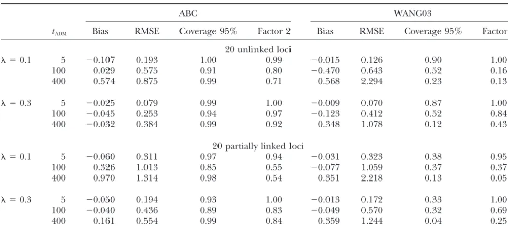
ad-TABLE 3
Effect of admixture time and partial linkage on the estimation of the admixture rateby the ABC andWang’s (2003) methods
ABC WANG03
tADM Bias RMSE Coverage 95% Factor 2 Bias RMSE Coverage 95% Factor 2
20 unlinked loci
⫽0.1 5 ⫺0.107 0.193 1.00 0.99 ⫺0.015 0.126 0.90 1.00
100 0.029 0.575 0.91 0.80 ⫺0.470 0.643 0.52 0.16
400 0.574 0.875 0.99 0.71 0.568 2.294 0.23 0.13
⫽0.3 5 ⫺0.025 0.079 0.99 1.00 ⫺0.009 0.070 0.87 1.00
100 ⫺0.045 0.253 0.94 0.97 ⫺0.123 0.412 0.52 0.84
400 ⫺0.032 0.384 0.99 0.92 0.348 1.078 0.12 0.43
20 partially linked loci
⫽0.1 5 ⫺0.060 0.311 0.97 0.94 ⫺0.031 0.323 0.38 0.95
100 0.326 1.013 0.85 0.55 ⫺0.077 1.059 0.37 0.37
400 0.970 1.314 0.98 0.54 0.351 2.218 0.13 0.05
⫽0.3 5 ⫺0.050 0.194 0.93 1.00 ⫺0.013 0.172 0.33 1.00
100 ⫺0.040 0.436 0.89 0.83 ⫺0.049 0.570 0.32 0.69
400 0.161 0.554 0.99 0.84 0.359 1.244 0.04 0.25
Simulated conditions are 106simulations; sample size, 100 genes. ⫽0.3,tDIV⫽5000,N0⫽N1⫽N2⫽NA⫽300.
mixture event occurred⬎100 generations ago, as shown to three times lower than that obtained from the ML method for the oldest admixture times (400 genera-by much smaller relative RMSE values, higher factor 2
scores, and much better coverage properties for the tions).
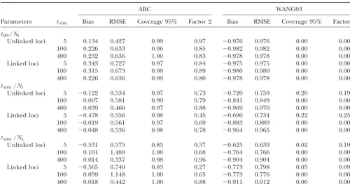
Estimation of divergence and admixture times:Wang’s ABC than for the ML method. For both unlinked and
partially linked loci, it is important to note that the ML method provides estimates of composite parameters such as divergence and admixture times scaled by popu-coverage of the ABC 95% confidence intervals is always
very good. On the other hand, confidence intervals pro- lation sizes; we report in Table 4 the corresponding parameters obtained from the ABC method. Because vided by the ML method become poorer with longer
admixture time for unlinked loci and are already much this ML method assumes that no mutation occurred since the divergence of the two parental populations, too low in the case of a recent admixture studied with
partially linked loci. The latter effect is certainly due to and thus that genetic differences between populations are due to a pure drift process, it leads to grossly under-the fact that under-the ML method assumes that under-the loci are
unlinked. As a consequence, loci that are correlated estimated divergence and admixture times and presents poor coverage property, even for recent admixtures. By provide similar information and tend to generate
thin-ner distributions because they overestimate the amount contrast, the divergence time scaled by parental popula-tion sizeN2(tDIV/N2) is only slightly overestimated with
of information in the data. This is not the case for the
ABC method since we explicitly model the correlation the ABC method from both linked and unlinked mark-ers, with good coverage and factor 2 scores. The admix-between partially linked markers in our simulations.
While 20 independent loci provide accurate estima- ture time scaled by parental population size N2 (tADM/ N2) is very well estimated by the ABC method when it
tion of admixture rates, there is a serious drop in the
quality of the ABC estimates based on partially linked is relatively ancient and is underestimated only by 12 and 48% on average when it is recent (five generations) markers, especially for very unequal contribution of the
parental population to the admixed population (i.e., ⫽ for unlinked and linked markers, respectively. This pa-rameter is also, to a lesser extent, well estimated by the 0.1). The decrease in ABC accuracy between linked and
unlinked loci is especially marked for older admixture ML method when admixture is recent. However, it is increasingly underestimated for older admixture times, events. Curiously, the ML method is less affected than
the ABC method by partial linkage, in the sense that its resulting in a virtual absence of coverage by the ML confidence intervals for admixture timesⱖ100 genera-performance evaluated by the relative bias and RMSE
does not degrade much when partially linked markers tions. Finally, the admixture time scaled by the admixed population sizeNA (tADM/NA) is only relatively well
esti-are used instead of independent markers. However,
TABLE 4
Effect of admixture time and partial linkage on the estimation of various composite parameters by the ABC andWang’s (2003) methods
ABC WANG03
Parameters tADM Bias RMSE Coverage 95% Factor 2 Bias RMSE Coverage 95% Factor 2
tDIV/N2
Unlinked loci 5 0.134 0.427 0.99 0.97 ⫺0.976 0.976 0.00 0.00
100 0.226 0.633 0.96 0.85 ⫺0.982 0.982 0.00 0.00
400 0.232 0.636 1.00 0.83 ⫺0.978 0.978 0.00 0.00
Linked loci 5 0.343 0.727 0.97 0.84 ⫺0.975 0.975 0.00 0.00
100 0.315 0.673 0.98 0.89 ⫺0.980 0.980 0.00 0.00
400 0.226 0.636 0.99 0.80 ⫺0.978 0.978 0.00 0.00
tADM/N2
Unlinked loci 5 ⫺0.122 0.534 0.97 0.73 ⫺0.720 0.759 0.20 0.19
100 0.007 0.581 0.99 0.79 ⫺0.841 0.849 0.00 0.00
400 0.039 0.460 0.97 0.88 ⫺0.969 0.970 0.00 0.00
Linked loci 5 ⫺0.478 0.556 0.98 0.45 ⫺0.690 0.734 0.22 0.23
100 ⫺0.019 0.561 0.97 0.69 ⫺0.883 0.889 0.00 0.00
400 ⫺0.048 0.536 0.98 0.78 ⫺0.964 0.965 0.00 0.00
tADM/NA
Unlinked loci 5 ⫺0.531 0.575 0.85 0.37 ⫺0.625 0.639 0.02 0.19
100 0.101 1.489 1.00 0.68 ⫺0.764 0.766 0.00 0.00
400 0.014 0.337 0.98 0.96 ⫺0.904 0.904 0.00 0.00
Linked loci 5 ⫺0.565 0.740 0.83 0.27 ⫺0.773 0.798 0.05 0.09
100 0.059 1.148 1.00 0.65 ⫺0.773 0.776 0.00 0.00
400 0.018 0.442 1.00 0.88 ⫺0.911 0.912 0.00 0.00
Simulated conditions are 106simulations, 20 loci, sample size 100 genes, ⫽0.3,tDIV⫽5000,N0⫽N
1⫽N2⫽NA⫽300.
method. The bias is large and negative for recent admix- Table 5, but follows the same pattern as 2) are very
well estimated even for old admixture times, while the ture events, and it becomes positive and associated with
a large RMSE fortADM⫽100; for older admixture times scaled size of the admixed population (A) is better
estimated with increasing admixture times. FortADM⫽
(tADM⫽400), the bias becomes very low and the relative
RMSE drops considerably. This pattern is probably due 400,Aestimation shows virtually no relative bias (⫺0.4%),
a relative RMSE (31%) becoming very similar to that of to the poor estimation of the admixed population size
NAfor short admixture times, since small or large popu- 2 (26%), and an excellent factor 2 score (98%). The
relatively flat posterior distribution ofA for recent
ad-lation sizes will not create very contrasting patterns of
diversity in a few generations, while they should lead to mixtures (five generations) underlines the absence of in-formation in the data for such recent events (Figure 3). On more contrasted patterns for longer evolutionary
peri-ods such as a few hundred generations. the other hand, the mean parameter of the geometric
distribution of the GSM modelPis well estimated with
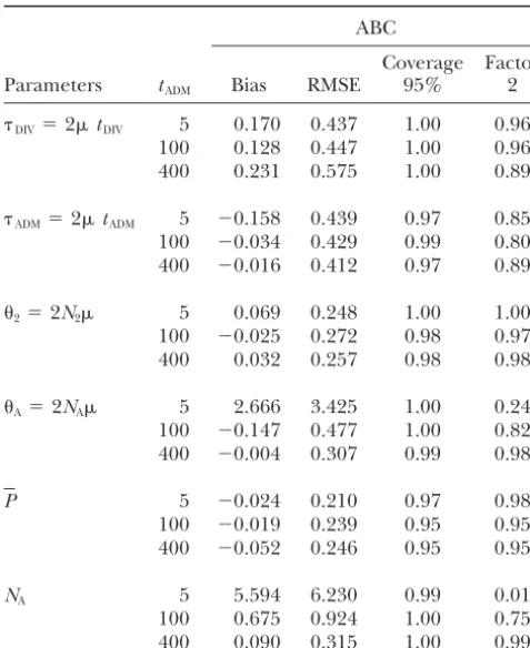
ABC estimation of mutation-scaled parameters: In
Table 5, we present results on the estimation of compos- 20 loci and does not seem much affected by the age of admixture. Finally, we note that the coverage of the ite parameters depending on mutations. These
parame-ters are computed only in the ABC method so that 95% confidence intervals is very good for all parameters and tends to be too conservative except forP.
comparison with Wang’s ML method is not possible.
The scaled divergence time DIV is relatively well esti- Application to a honeybee data set: This honeybee
data set has been previously described and analyzed in mated for short admixture time (17% of positive bias)
and its relative RMSE is only slightly increased with Choisy et al. (2004). The population under study is located in Courmayeur at the extreme north of the longer admixture times, resulting in a small drop (96–
89%) for the factor 2 score. The scaled admixture time Aosta valley (northwestern Italy) and represented by a sample of 33 worker bees (one per colony). It is consid-ADMis increasingly better estimated with older
admix-ture events, in keeping with results obtained for the ered an artificially admixed population between two different subspecies ofApis mellifera, the West-European scale parametertADM/N2. The relatively poor recovery of
this parameter for recent admixture is also visible in black honeybee (A. m. mellifera) and the Italian yellow honeybee (A. m. ligustica). The two parental populations Figure 3, where the posterior distribution ofADMis not
TABLE 5 mates reach 7.2–8.3.A. m. ligustica and A. m. mellifera
have long been considered as two very distinct
subspe-Effect of admixture time on the estimation of various
cies of honeybees. At the end of the 1980s (e.g.,Ruttner composite parameters depending on the mutation
1988), the current theory based on paleogeography and
rate, as well as the admixed population
size (NA) by the ABC method morphometry was that the Quaternary ice ages were
responsible for the separation of the two subspecies,
ABC so the divergence time was estimated atⵑ50,000 years
before present (BP). However, mitochondrial studies
Coverage Factor
Parameters tADM Bias RMSE 95% 2 showed that these two subspecies belonged to two highly
divergent lineages having probably divergedⵑ1 million
DIV⫽2tDIV 5 0.170 0.437 1.00 0.96
years ago (Garneryet al.1992). Quite recently,Franck
100 0.128 0.447 1.00 0.96
et al. (2000) showed that the subspecies ligustica had
400 0.231 0.575 1.00 0.89
actually a hybrid origin using a much larger sample of
ADM⫽2tADM 5 ⫺0.158 0.439 0.97 0.85 colonies, and that its genetic pool was a mixture of 100 ⫺0.034 0.429 0.99 0.80 two lineages: the M lineage constituted mainly by the
400 ⫺0.016 0.412 0.97 0.89
melliferasubspecies and the C lineage encompassing the South-European subspeciescarnicaandcecropia, as well
2⫽2N2 5 0.069 0.248 1.00 1.00
as the Asiancaucasica. According toFrancket al.(2000),
100 ⫺0.025 0.272 0.98 0.97
400 0.032 0.257 0.98 0.98 the admixture might have taken place any time after the Riss period (in the last 130,000 years), and it is
A⫽2NA 5 2.666 3.425 1.00 0.24 probably rather ancient. The estimated divergence time
100 ⫺0.147 0.477 1.00 0.82
could thus not correspond to the separation of the C
400 ⫺0.004 0.307 0.99 0.98
and M lineages, but rather to the time when the admixed
ligusticaand themelliferasubspecies were last separated.
P 5 ⫺0.024 0.210 0.97 0.98
100 ⫺0.019 0.239 0.95 0.95 If we admit the timing given byFrancket al.(2000), a
400 ⫺0.052 0.246 0.95 0.95 sensible estimate would be some time during the last
ice age (which at maximum occurred 22,000–14,000
NA 5 5.594 6.230 0.99 0.01
years BP), when honeybee populations were restricted
100 0.675 0.924 1.00 0.75
to southern Mediterranean refuges (namely the Iberian
400 0.090 0.315 1.00 0.99
and Italian peninsulas, respectively). Taking population sizes as above, we get divergence time estimate intervals of 150–500 years with Wang’s ML estimates and 14,400– tany,n⫽49) and a sample ofA. m. ligusticafrom Forli
33,200 years with our ABC approach. Wang’s ML esti-(Emilia-Romania,n ⫽19), an area of intensive queen
mates for the time of divergence of the two subspecies rearing for exportation. All sampled honeybees were
hence appear clearly underestimated, while the ABC characterized at eight microsatellite loci, and the
admix-method gives estimates much more compatible with ture coefficient of the Courmayeur sample has already
our current knowledge of the evolutionary history of been estimated by six different methods (seeChoisyet
European honeybee populations.
al.2004 for more details). Such estimates of the
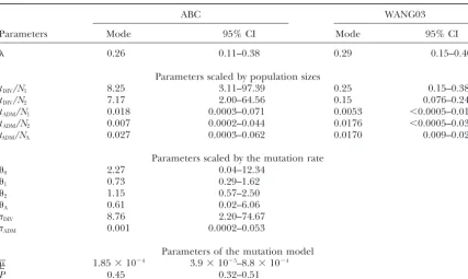
propor-The ABC approach also allows the estimation of sev-tion ofA. m. melliferagenes in the Courmayeur genetic
eral other parameters not estimated by Wang’s ML pool ranged from 0.195 to 0.371 (Choisyet al.2004).
method (Table 6), such as the mutation scaled popula-Table 6 shows that our ABC estimate (0.259) is well
tion sizes (’s) and the times of divergenceDIVor
admix-within this range, as is Wang’s ML estimate (0.287).
tureADM. Using the mode of the posterior distribution
These two methods also agree in their estimates of the
of the average mutation rate (1.85⫻ 10⫺4), we obtain
time of admixture, which isⵑ0.01–0.02 in units ofN.
an estimate of 23,665 generations (47,330 years) for the Considering that effective population sizes (in number
divergence time and 26 generations (52 years) for the of gene copies) in European honeybee subspecies are
time of admixture. Both values are in excellent agree-of the order agree-of 1000–2000 [Estoupet al.’s (1995) Table
ment with those mentioned above and with other studies 4], this implies a rather recent admixture of 10–40
gen-(Ruttner 1988;Francket al2000). The average geo-erations, corresponding to 20–80 years (using an
aver-metric coefficientPof the GSM mutation model is very age generation time of 2 years for the queens). This is
high (0.446) and very close to the upper bound of our in good agreement with the development of the Italian
prior distribution (Table 1). This extreme value implies queen selling industry in Europe in the middle of the
a surprisingly large proportion of mutations leading to twentieth century. As expected from our previous
simu-non-single-step mutations (precisely 0.446;Estoupet al.
lations (Table 4), the two methods provide very different
2002). This probably results from the fact that this data estimates of the time of divergence of the two parental
set does not fit well to the modeled scenario. More populations scaled by effective population sizes. Wang’s
TABLE 6
Estimated parameters of the admixture model for the Courmayeur honeybee sample
ABC WANG03
Parameters Mode 95% CI Mode 95% CI
0.26 0.11–0.38 0.29 0.15–0.40
Parameters scaled by population sizes
tDIV/N1 8.25 3.11–97.39 0.25 0.15–0.38
tDIV/N2 7.17 2.00–64.56 0.15 0.076–0.242
tADM/N1 0.018 0.0003–0.071 0.0053 ⬍0.0005–0.019
tADM/N2 0.007 0.0002–0.044 0.0176 ⬍0.0005–0.035
tADM/NA 0.027 0.0003–0.062 0.0170 0.009–0.025
Parameters scaled by the mutation rate
0 2.27 0.04–12.34
1 0.73 0.29–1.62
2 1.15 0.57–2.50
A 0.61 0.02–6.06
DIV 8.76 2.20–74.67
ADM 0.001 0.0002–0.053
Parameters of the mutation model
1.85⫻10⫺4 3.9⫻10⫺5–8.8⫻10⫺4
P 0.45 0.32–0.51
Simulated conditions are 106simulations, prior distributions are as in Table 1. CI, credibility interval.
population (ligustica) may have widened the distribution gests that the absolute size of old admixed populations could be well estimated under our framework. This is of allele lengths in the corresponding sample, forcing
the analysis to increase the average length of the muta- probably because our method implicitly attempts to re-construct the genetic composition of the admixed popu-tion steps to cope with this widened allelic distribupopu-tion.
lation at the time of admixture, which puts us into a framework very similar to a temporal spacing of samples,
DISCUSSION which is the ideal situation for estimating population
sizes independently from mutation rates (e.g.,
William-This study shows that the ABC framework allows a
sonandSlatkin1999;Andersonet al.2000;Berthier
fine analysis of an admixture model, providing very
satis-et al.2002). factory estimates of admixture rate (), mutation-scaled
Compared to Wang’s ML method, our ABC approach parental population sizes (1 and 2), and divergence
shows comparable performance for the estimation of time DIV, as well as those of the mutation model.
Esti-the admixture coefficient when admixture is recent, but mates of scaled ancestral population size (0) are usually
leads to increasingly better relative results when the poor, and those of the admixed population size (A)
admixture time is older. We attribute this better perfor-are good only when the admixture time is large. The
mance to the specific handling of mutations, which can-mutation-scaled admixture time (ADM) is itself very well
not be neglected when admixture time is ancient. How-estimated when the admixture event is relatively old
ever, to estimate admixture coefficients, methods based (100 or more generations), while it leads to reasonable
on a pure drift process are not handicapped by muta-point estimates but large credible intervals when it is
tions having occurred before the admixture, as they very recent. Unscaled parameters, such as raw
popula-merely result in larger diversity in parental populations. tion sizes and raw divergence and admixture times, were
Drift-based (like current likelihood-based) methods seem usually not estimated as well as the scaled parameters
also to better deal with short divergence time between (results not shown), as they do not have independent
parental populations (e.g., 200 generations instead of and contrasting effects on genetic diversity. However,
5000) than does our ABC procedure when the admix-it is worth noting that the size of the admixed population
ture is recent (results not shown). However, this
advan-NAwas very well estimated in the case of old admixture
tage is valid only for recent admixtures (e.g.,⬍50 genera-events (i.e., 400 generations). As shown in Table 5, the
tions). Another advantage of the present ABC approach relative bias onNAis indeed⬍10% when the admixture
is its ability to correctly estimate other parameters of time is 400 generations, while it was ⵑ560% for an
times. These parameters are often as important as the of simulated summary statistics from which the estima-tion procedure proceeds (e.g., 106iterations). However,
admixture coefficient itself. The better performance of
our approach is probably linked to the fact that we are reasonable point estimates can be obtained using much fewer simulations and hence shorter computation times using information not specifically handled by Wang’s
ML method, such as information on patterns of LD and (e.g., 105 iterations). It seems reasonable to anticipate
that progress in simulation algorithms and higher com-mutations, as well as range of allele size. Moreover, our
ABC approach allows us to explicitly include informa- puting power will be available in future years, promoting the ABC method as the method of choice for analyzing tion on partial linkage between markers, so that, in
contrast to Wang’s ML method, accurate confidence complex evolutionary scenarios and, more specifically in the context of the present study, for old admixture intervals are also obtained in this case.
While the admixture model analyzed here (with a models in which mutation cannot be neglected or when nonindependent markers are available.
hybrid population and two isolated parental
popula-tions at mutation-drift equilibrium) corresponds to the We are grateful to Loune`s Chikhi and Mark Beaumont for their standard model assumed by most methods of estimation comments on the manuscript. L.E. was supported by Swiss National Science Foundation grant 3100A0-100800, as well as a grant from the
of admixture coefficients (e.g., Long1991;Bertorelle
Institut de la Recherche Agronomique during his 2004 sabbatical visit
andExcoffier1998;Wang2003;Choisyet al.2004),
at the Centre de Biologie et de Gestion des Populations. This study
real models of admixture may be much more complex.
was also partially supported by a grant from the French Bureau des
They may indeed involve: (i) more than two source Ressources Ge´ne´tiques. populations (Dupanloup andBertorelle2001); (ii)
some regular (and thus not instantaneous) admixture
events over relatively long periods (reviewed inChakra- LITERATURE CITED
borty 1986); (iii) subdivided source populations, so
Anderson, E. C., andE. A. Thompson, 2002 A model-based method
that the actual parental population is only partially sam- for identifying species hybrids using multilocus genetic data.
Ge-netics160:1217–1229.
pled; and (iv) parental population(s) that are not at
Anderson, E. C., E. G. Williamson andE. A. Thompson, 2000
mutation-drift equilibrium, due to population size
fluc-Monte Carlo evaluation of the likelihood forNefrom temporally tuations or introgression event(s) in a more or less re- spaced samples. Genetics156:2109–2118.
Barton, N. H., 2001 The role of hybridization in evolution. Mol.
cent past. The ABC approach has the potential to assess
Ecol.10:551–568.
the effect of such deviations from the standard
admix-Beaumont, M. A., W. ZhangandD. J. Balding, 2002 Approximate
ture model on parameter estimations since the ratio of Bayesian computation in population genetics. Genetics 162:
2025–2035.
acceptance under two alternative models approximates
Berthier, P., M. A. Beaumont, J. M. CornuetandG. Luikart, 2002
the Bayes factor (e.g.,Estoupet al.2004;Pritchardet
Likelihood-based estimation of the effective population size using
al.1999). Such quantitative model comparisons could temporal changes in allele frequencies: a genealogical approach.
Genetics160:741–751.
be particularly useful in the present evolutionary
con-Bertorelle, G., andL. Excoffier, 1998 Inferring admixture
pro-text to assess the likelihood of different deviations from
portions from molecular data. Mol. Biol. Evol.15:1298–1311.
the standard admixture model and hence learn more Chakraborty, R., 1986 Gene admixture in human populations:
models and predictions. Yearb. Phys. Anthropol.29:1–43.
about the admixture process that produced the
ob-Chakraborty, R., andK. M. Weiss, 1988 Admixture as a tool for
served data set and potentially consider more realistic
finding linked genes and detecting that difference from allelic
models for parameter estimation. association between loci. Proc. Natl. Acad. Sci. USA85:9119–
9123.
A general feature of the ABC methods that should
Chikhi, L., M. W. BrufordandM. A. Beaumont, 2001 Estimation
be underlined here is their ability to assess their
perfor-of admixture proportions: a likelihood-based approach using
mance at almost no extra computation cost. Other esti- Markov chain Monte Carlo. Genetics158:1347–1362.
Choisy, M., P. FranckandJ. M. Cornuet, 2004 Estimating
admix-mation methods generally require a validation step,
ture proportions with microsatellites: comparison of methods
which includes the time-consuming analysis of
indepen-based on simulated data. Mol. Ecol.13:955–968.
dently produced simulated data sets (e.g.,Choisyet al. Dawson, K. J., andK. Belkhir, 2001 A Bayesian approach to the
identification of panmictic populations and the assignment of
2004), whereas this is intrinsic in the ABC approach (cf.
individuals. Genet. Res.78:59–77.
Figure 2). As a matter of fact, the same ABC process
Dupanloup, I., andG. Bertorelle, 2001 Inferring admixture
pro-used to build the reference table can be derived to portions from molecular data: extension to any number of
paren-tal populations. Mol. Biol. Evol.18:672–675.
produce test data sets with known values of parameters.
Dupanloup, I., G. Bertorelle, L. ChikhiandG. Barbujani, 2004
The same rejection and regression steps can then be
Estimating the impact of prehistoric admixture on the genome
applied to these data sets to produce estimates of param- of Europeans. Mol. Biol. Evol.21:1361–1372.
Ellegren, H., 2004 Microsatellites: simple sequences with complex
eters that can be compared to their known true values.
evolution. Nat. Rev. Genet.5:435–445.
It is therefore relatively quick and easy to evaluate the
Estoup, A., M. Beaumont, F. Sennedot, C. MoritzandJ.-M. Cor-performance of the method for any subset of the param- nuet, 2004 Genetic analysis of complex demographic scenarios:
spatially expanding populations of the cane toad, Bufo marinus.
eter space under a given model. The applicability of
Evolution58:2021–2036.
the ABC method to particular cases should, however,
Estoup, A., andS. M. Clegg, 2003 Bayesian inferences on the recent
depend on available computer power, as a few days of island colonization history by the bird Zosterops lateralis lateralis.
Mol. Ecol.12:657–674.
Estoup, A., L. Garnery, M. SolignacandJ. M. Cornuet, 1995 Mi- Goldstein, D. B., A. Ruiz Linares, L. L. Cavalli-SforzaandM. W.
crosatellite variation in honey bee (Apis mellifera L.) populations: Feldman, 1995 Genetic absolute dating based on microsatel-hierarchical genetic structure and test of the infinite allele and lites and the origin of modern humans. Proc. Natl. Acad. Sci. stepwise mutation models. Genetics140:679–695. USA92:6723–6727.
Estoup, A., C. R. Largiader, J. M. Cornuet, K. Gharbi, P. Presa Hudson, R. R., 2002 Generating samples under a Wright-Fisher
et al., 2000 Juxtaposed microsatellite systems as diagnostic mark- neutral model of genetic variation. Bioinformatics18:337–338. ers for admixture: an empirical evaluation with brown trout Laval, G., and L. Excoffier, 2004 SIMCOAL 2.0: a program to (Salmo trutta) as model organism. Mol. Ecol.9:1873–1886. simulate genomic diversity over large recombining regions in a
Estoup, A., I. J. Wilson, C. Sullivan, J. M. CornuetandC. Moritz, subdivided population with a complex history. Bioinformatics20: 2001 Inferring population history from microsatellite and en- 2485–2487.
zyme data in serially introduced cane toads,Bufo marinus. Genet- Long, J. C., 1991 The genetic structure of admixed populations. ics159:1671–1687. Genetics127:417–428.
Estoup, A., P. Jarne and J. M. Cornuet, 2002 Homoplasy and Marjoram, P., J. Molitor, V. PlagnolandS. Tavare, 2003 Markov mutation model at microsatellite loci and their consequences for chain Monte Carlo without likelihoods. Proc. Natl. Acad. Sci. population genetics analysis. Mol. Ecol.11:1591–1604. USA100:15324–15328.
Falush, D., M. StephensandJ. K. Pritchard, 2003 Inference of Pollock, D. D., A. Bergman, M. W. FeldmanandD. B. Goldstein, population structure using multilocus genotype data: linked loci 1998 Microsatellite behavior with range constraints: parameter and correlated allele frequencies. Genetics164:1567–1587. estimation and improved distances for use in phylogenetic
recon-Feldman, M. W., A. Bergman, D. D. PollockandD. B. Goldstein, struction. Theor. Popul. Biol.53:256–271.
1997 Microsatellite genetic distances with range constraints: an- Pritchard, J., M. Seielstad, A. Perez-LezaunandM. Feldman, alytic description and problems of estimation. Genetics145:207– 1999 Population growth of human Y chromosomes: a study of 216.
Y chromosome microsatellites. Mol. Biol. Evol.16:1791–1798.
Franck, P., L. Garnery, G. Celebrano, M. Solignac and J. M. Pritchard, J. K., M. StephensandP. Donnelly, 2000 Inference Cornuet, 2000 Hybrid origins of honeybees from Italy (Apis
of population structure using multilocus genotype data. Genetics mellifera ligustica) and Sicily (A. m. sicula). Mol. Ecol.9:907–921.
155:945–959.
Fu, Y. X., andW. H. Li, 1997 Estimating the age of the common
Roberts, D., andR. Hiorns, 1965 Methods of analysis of the genetic ancestor of a sample of DNA sequences. Mol. Biol. Evol. 14:
composition of a hybrid population. Hum. Biol.37:38–43. 195–199.
Ruttner, F., 1988 Biogeography and Taxonomy of Honeybees.
Springer-Gaggiotti, O. E., F. Jones, W. M. Lee, W. Amos, J. Harwoodet al.,
Verlag, Berlin. 2002 Patterns of colonization in a metapopulation of grey seals.
Tavare´, S., D. Balding, R. C. GriffithsandP. Donnely, 1997 In-Nature416:424–427.
ferring coalescence times from DNA sequence data. Genetics
Gaggiotti, O. E., S. P. Brooks, W. AmosandJ. Harwood, 2004
145:505–518. Combining demographic, environmental and genetic data to test
Wang, J., 2003 Maximum-likelihood estimation of admixture pro-hypotheses about colonization events in metapopulations. Mol.
portions from genetic data. Genetics164:747–765. Ecol.13:811–825.
Weir, B. S., andC. C. Cockerham, 1984 Estimating F-statistics for
Garnery, L., J. M. CornuetandM. Solignac, 1992 Evolutionary
the analysis of population structure. Evolution38:1358–1370. history of the honey bee Apis mellifera inferred from
mitochon-Williamson, E. G., andM. Slatkin, 1999 Using maximum likeli-drial DNA analysis. Mol. Ecol.1:145–154.
hood to estimate population size from temporal changes in allele
Garza, J. C., andE. G. Williamson, 2001 Detection of reduction
in population size using data from microsatellite loci. Mol. Ecol. frequencies. Genetics152:755–761.
10:305–318. Wilson, I. J., andD. J. Balding, 1998 Genealogical inference from
Garza, J. C., M. SlatkinandN. B. Freimer, 1995 Microsatellite microsatellite data. Genetics150:499–510.
allele frequencies in humans and chimpanzees, with implications Zhivotovsky, L. A., M. W. FeldmanandS. A. Grishechkin, 1997 for constraints on allele size. Mol. Biol. Evol.12:594–603. Biased mutations and microsatellite variation. Mol. Biol. Evol.
Goldstein, D. B., andD. D. Pollock, 1997 Launching microsatel- 14:926–933. lites: a review of mutation processes and method of phylogenetic