ABSTRACT
SMITH, JUSTIN WADE. Model Based Fault Locating on Distribution Feeders. (Under the direction of Dr. Mesut E Baran.)
As electric power systems grow in complexity and size, ensuring system reliability and con-tinuity has become a major concern. Failure to locate faults quickly can result in prolonged outage times, customer safety concerns and lost revenues. Over the past few decades distri-bution networks have evolved into large and complex networks capable of carrying thousands of customers. As of late, utilities have displayed particular interest in distribution fault lo-cation technology to reduce such widespread impacts. This thesis aims to develop a modern distribution fault locating algorithm.
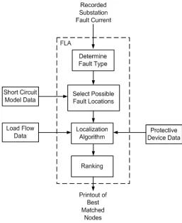
The proposed fault locating algorithm is a model based algorithm that uses a short circuit model of the feeder to locate the fault. In the short circuit model, a fault is placed at every node and the observed fault current at the substation is recorded in tabular format. During an actual fault condition, the algorithm compares the recorded fault current at the substation to the short circuit modelling data. This comparison allows the fault locator to identify the exact node in the network that is faulty.
In many cases, the short circuit model will indicate that there are several unique nodes with the same fault current magnitude. This problem is overcome with a proposed sub-algorithm called the localization algorithm. This algorithm uses protective device data and load flow data to determine the protective device that has interrupted the fault. By knowing the protective device that has interrupted the fault, the fault can be localized to a specific region of the network.
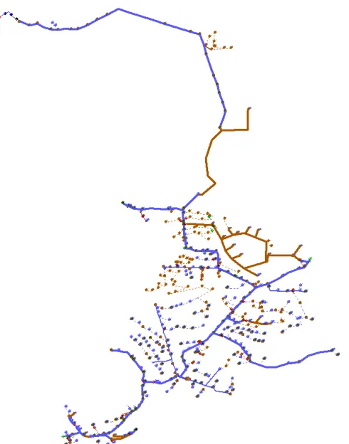
To test the fault locating algorithm, four different test cases are proposed. Three test cases are performed using a Progress Energy Carolinas feeder model. Detailed fuse, recloser and substation breaker models are inserted into the feeder model to test popular protective schemes such as fuse saving and fuse blowing. Finally, the Stewart Street 12.47kV feeder is tested using DEW models provided by Allegheny Power. The Stewart Street feeder is much larger than the Progress Energy Carolinas feeder model and contains hundreds of nodes and tapped loads.
Model Based Fault Locating on Distribution Feeders
by
Justin Wade Smith
A thesis submitted to the Graduate Faculty of North Carolina State University
in partial fulfillment of the requirements for the Degree of
Master of Science
Electrical Engineering
Raleigh, North Carolina
2013
APPROVED BY:
Dr. Subhashish Bhattacharya Dr. Srdjan Lukic
DEDICATION
To my parents Jeffrey W. Smith and Cindy A. Smith. Without you, none of this would have been possible. You gave me strength when I had nothing left and encouragement when I
couldn’t carry on. This one is for you.
To my grandfather Harold W. Smith who never got to see my thesis completed.
BIOGRAPHY
ACKNOWLEDGEMENTS
I would like to thank my advisor Dr. Mesut E. Baran, and my other committee members, Dr. Subhashish Bhattacharya and Dr. Srdjan Lukic.
I would also like to acknowledge Larry Alesi at Schweitzer Engineering Laboratories(SEL) for his guidance. Much of my knowledge in the field of power system protection can be attributed to the mentorship and dedication of Mr. Alesi. He is true mentor and friend.
I would like to thank Bette Gray of Rodanthe, N.C. for helping me chase my dreams. My family could not have been blessed with a greater friend.
I would like to thank my friends Nick Parks and Jon McDonald. Their support and friendship led me to success.
TABLE OF CONTENTS
LIST OF TABLES. . . ix
LIST OF FIGURES . . . xi
Chapter 1 Introduction . . . 1
1.1 Introduction . . . 1
1.2 Challenges of Distribution Fault Locating . . . 1
1.3 Proposed Solution: Model Based Algorithm . . . 2
1.4 Glossary of Terms . . . 4
Chapter 2 Modern Distribution Fault Locating Algorithms . . . 5
2.1 Introduction to Distribution Fault Locating Algorithms . . . 5
2.2 Technique with Two-port Network Section Representation(Das Method) . . . 5
2.2.1 Overview of Das Method . . . 6
2.2.2 Data Acquisition . . . 6
2.2.3 Fault Detection and Classification . . . 6
2.2.4 Developing an Equivalent Radial Network . . . 10
2.2.5 Load Modelling . . . 11
2.2.6 Estimating nodal pre-fault voltages and currents . . . 12
2.2.7 Estimating Voltages and Currents at the Remote End and at the Fault . 15 2.2.8 Calculating the Distance to the Fault: Single Line to Ground . . . 18
2.2.9 Assessment of the Das Algorithm: Advantages and Disadvantages . . . . 19
2.3 Girgis Apparent Impedance Method . . . 21
2.3.1 Overview of Girgis Method . . . 21
2.3.2 Direct Determination of Distance to the Fault . . . 21
2.3.3 Assessment of the Girgis Algorithm: Advantages and Disadvantages . . . 26
2.4 Fault Locating using Digital Fault Recorder Data(Saha Algorithm) . . . 27
2.4.1 Overview of Saha Method . . . 27
2.4.2 Fault Loop Impedance Determination . . . 27
2.4.3 Determination of the Faulty Node . . . 30
2.4.4 Distance to the Fault . . . 34
2.4.5 Assessment of the Saha Algorithm: Advantages and Disadvantages . . . . 38
2.5 Conclusion . . . 39
Chapter 3 Model Based Fault Locating . . . 40
3.1 Introduction . . . 40
3.2 Sampled Data Conditioning . . . 41
3.3 Steady State Fault Current Extraction . . . 43
3.4 Fault Tables . . . 44
3.4.1 Sliding Fault Resolution . . . 46
3.4.2 Selecting Possible Fault Locations from Fault Tables . . . 47
3.4.4 Calculation of Fault Currents in the Fault Table: Fault Resistance . . . . 49
3.5 Localization Techniques . . . 49
3.5.1 Localization Using Protective Devices . . . 50
3.5.2 Zones of Protection . . . 52
3.5.3 Localization using Fuse Characteristics . . . 53
3.5.4 Estimating Fault Current Through the Fuse . . . 56
3.6 Localization using Load-Flow Rejection . . . 58
3.6.1 Calculating Best Matched Device from Load Flow Rejection . . . 59
3.7 Combining Localization Data for Best Match . . . 61
3.7.1 Final Ranking of Each Possibility . . . 62
3.8 Localization Flow Chart . . . 64
Chapter 4 Fault Locator Test Results . . . 65
4.1 Introduction to the Notional Feeder, Stewart Street Feeder and Test Cases . . . . 65
4.2 Notional Feeder Fault Tables and Short Circuit Data . . . 66
4.3 Test Case 1: Notional Feeder Testing With No Localization . . . 67
4.3.1 Introduction: Test Conditions and Procedure . . . 67
4.3.2 FLA Testing for Line-to-Ground Faults . . . 67
4.3.3 FLA Testing for Line-to-Line Faults . . . 68
4.3.4 Test Case 1 Results: . . . 69
4.4 Test Case 2: Localization using Load Flow and Protective Devices . . . 70
4.4.1 Introduction: Test Conditions and Procedures . . . 71
4.4.2 FLA Testing for Line-to-Ground Faults . . . 71
4.4.3 A-Ground Fault at Node 17 . . . 72
4.4.4 A-Ground Fault at Node 7 . . . 75
4.4.5 Limitations of the Localization Algorithm: A-Ground Fault at Node 16 . 77 4.5 Test Case 3: Fault Locating on Fuse Saving or Fuse Blowing Schemes . . . 79
4.5.1 Introduction: Notional Feeder with Fuse Blowing Coordination . . . 79
4.5.2 Introduction: Fuse Blowing Scheme Test Conditions . . . 80
4.5.3 FLA Testing for Line-to-Ground Faults: Fuse Blowing . . . 80
4.5.4 Line-to-Ground Fault at Node 17 . . . 80
4.5.5 Line-to-Ground Fault at Node 6 . . . 83
4.5.6 Introduction: Notional Feeder with Fuse Saving Coordination . . . 85
4.5.7 Introduction: Fuse Saving Scheme Test Conditions . . . 85
4.5.8 FLA Testing for Line-to-Ground Faults: Fuse Saving . . . 85
4.5.9 Line-to-Ground Fault at Node 10 . . . 86
4.5.10 Line-to-Ground Fault at Node 6 . . . 88
4.5.11 Limitations of the FLA on Fuse Blowing or Fuse Saving Coordinated Feeders . . . 90
4.6 Notional Feeder Test Results Summary . . . 91
4.6.1 Test Case 1 Summary . . . 91
4.6.2 Test Case 2 Summary . . . 91
4.6.3 Test Case 3 Summary . . . 91
4.7 Test Case 4: Fault Locating on Large Scale Feeders . . . 93
4.7.2 Introduction: Test Conditions and Procedures . . . 94
4.7.3 Fault Tables for the Stewart Street Feeder . . . 95
4.7.4 Load Flow Analysis on the Stewart Street 12.47kV Feeder . . . 95
4.7.5 MATLAB Fault Modelling of the Stewart Street 12.47kV Feeder . . . 96
4.7.6 Fault at Pole P4622 on the Stewart Street 12.47kV Feeder . . . 98
4.7.7 FLA Test Results for P4622 Fault . . . 103
4.7.8 Fault at Pole P4266 on the Stewart Street 12.47kV Feeder . . . 105
4.7.9 FLA Test Results for P4266 Fault . . . 109
4.7.10 FLA Test Results Summary for Stewart Street Feeder . . . 111
4.8 Sensitivity Analysis: System Load Perturbations . . . 112
4.8.1 Introduction: Sensitivity Analysis . . . 112
4.8.2 System Load Perturbations: Test Conditions and Procedures . . . 112
4.8.3 System Load Perturbations on Test Case 1-No Localization . . . 114
4.8.4 System Load Perturbations on Test Case 2 . . . 116
4.8.5 System Load Perturbations on Test Case 3-Fuse Saving . . . 118
4.8.6 System Load Perturbations on Test Case 3-Fuse Blowing . . . 120
Chapter 5 FLA Testing Conclusions . . . .122
References. . . .124
Appendices . . . .126
Appendix A Notional Feeder Load Flow Data . . . 127
A.1 Notional Feeder Real Power Flow Data . . . 127
A.2 Notional Feeder Reactive Power Flow Data . . . 129
A.3 12kV Capacitor Bank Data . . . 130
A.4 Transformer Bank Data . . . 130
A.5 Source Impedance Data . . . 130
A.6 Line Impedance Data . . . 131
A.6.1 Positive Sequence Line Impedance Data . . . 131
A.6.2 Negative Sequence Line Impedance Data . . . 132
A.6.3 Zero Sequence Line Impedance Data . . . 133
A.6.4 Positive and Zero Sequence Shunt Capacitance Data . . . 134
A.7 Relay Settings and Fuse Characteristics . . . 135
A.8 Fuse Characteristics . . . 136
Appendix B Modelling of the Notional Feeder using MATLAB . . . 138
B.1 Introduction . . . 138
B.2 Modelling of Lines . . . 138
B.3 Modelling of System Loads . . . 141
B.3.1 Load Modelling Under Fault Conditions . . . 142
B.4 Modelling of Sources . . . 143
B.5 Modelling of Capacitor Banks . . . 143
B.6 Modelling of Multi-Winding Transformers . . . 144
Appendix C Distribution Fault Analysis . . . 147
C.1 System Fault Currents and Voltages via Numerically Computed Thevenin Equivalents and Sensitivity Matrices . . . 147
C.1.1 Thevanin’s Theorem and Superposition Principle . . . 148
C.1.2 Pre-Fault and Faulted Systems in DEW . . . 151
C.1.3 Forming the Phase Thevanin Matrix . . . 155
C.1.4 System Fault Characteristics . . . 158
C.1.5 3-Phase Faults . . . 160
C.1.6 Phase-to-Phase-Ground Faults . . . 162
C.1.7 Phase-to-Phase Faults . . . 164
C.1.8 Single Line-to-Ground Faults . . . 166
C.2 Verification of DEW Fault Current Calculation: Example Feeder . . . 167
C.2.1 Validation with MATLAB Simulink Model . . . 173
Appendix D Supplemental FLA Simulation Results for Stewart Street 12.47kV Feeder174 D.1 Pole P4622 Supplemental Recorded Results . . . 174
LIST OF TABLES
Table 3.1 Fault Table for Figure 3.7 . . . 46
Table 3.2 Increased Resolution Fault Table for Figure 3.7 . . . 47
Table 4.1 Notional Feeder Fault Table for SLG Faults on A Phase. . . 66
Table 4.2 Line-to-Ground Simulation Results for Test Case 1 . . . 69
Table 4.3 Phase-to-Phase Fault Simulation Results for Test Case 1 . . . 69
Table 4.4 Percent Mismatch Table for Protective Device Localization. . . 74
Table 4.5 Percent Mismatch Table for Load Rejection Localization . . . 74
Table 4.6 Percent Mismatch Table for Protective Device Localization . . . 76
Table 4.7 Percent Mismatch Table for Load Rejection Localization . . . 77
Table 4.8 Percent Mismatch Table for Protective Device Localization . . . 82
Table 4.9 Percent Mismatch Table for Load Rejection Localization . . . 82
Table 4.10 Percent Mismatch Table for Protective Device Localization . . . 84
Table 4.11 Percent Mismatch Table for Load Rejection Localization . . . 84
Table 4.12 Percent Mismatch Table for Protective Device Localization . . . 87
Table 4.13 Percent Mismatch Table for Load Rejection Localization . . . 87
Table 4.14 Percent Mismatch Table for Protective Device Localization . . . 89
Table 4.15 Percent Mismatch Table for Load Rejection Localization . . . 89
Table 4.16 Substation Bus Load Flow Solution for Stewart Street Feeder. . . 96
Table 4.17 Pre-Fault Load Flow Values . . . 98
Table 4.18 Fault Analysis Calculated Parameters . . . 100
Table 4.19 MATLAB Model Parameters . . . 102
Table 4.20 Pre-Fault DEW Load Flow Values . . . 107
Table 4.21 Success-Failure Rate on Node 10, Test Case 1(No Localization) . . . 114
Table 4.22 Success-Failure Rate on Node 17, Test Case 1(No Localization) . . . 115
Table 4.23 Success-Failure Rate on Node 4, Test Case 1(No Localization) . . . 115
Table 4.24 Success-Failure Rate on Load Perturbation Test for Node 10 Fault . . . . 117
Table 4.25 Success-Failure Rate on Load Perturbation Test for Node 17 Fault . . . . 117
Table 4.26 Success-Failure Rate on Load Perturbation Test for Node 10 Fault with Fuse Saving Feeder Coordination. . . 118
Table 4.27 Success-Failure Rate on Load Perturbation Test for Node 17 Fault with Fuse Saving Feeder Coordination. . . 119
Table 4.28 Success-Failure Rate on Load Perturbation Test for Node 10 Fault with Fuse Blowing Feeder Coordination. . . 120
Table 4.29 Success-Failure Rate on Load Perturbation Test for Node 17 Fault with Fuse Blowing Feeder Coordination. . . 121
Table A.1 Relay Settings for Substation Breaker A and Substation Breaker B . . . . 135
Table A.2 Relay Settings for Recloser A and Recloser B . . . 135
Table C.1 Fault types and their frequency of occurrence[23]. . . 159
Table C.3 Current Results of DEW vs. MATLAB Script . . . 169
Table C.4 MATLAB Simulink Fault Current Results . . . 173
Table D.1 Other Likely Fault Possibilities for P4622 . . . 177
LIST OF FIGURES
Figure 1.1 12kV Radial Feeder. . . 2
Figure 1.2 FLA High Level Overview. . . 3
Figure 2.1 Radial Distribution Feeder[25]. . . 7
Figure 2.2 Flow Chart for Determining fault type[25]. . . 8
Figure 2.3 Line section Bus M and Bus R. . . 9
Figure 2.4 Radial Distribution Feeder[25]. . . 10
Figure 2.5 Voltage and Current relationship between M and R[25]. . . 13
Figure 2.6 Consolidated loads at the remote end, Node N[25]. . . 15
Figure 2.7 Fault between Nodesx and x+ 1(=y)[25]. . . 16
Figure 2.8 Fault locator load model as constant impedance with system load model as constant power [8]. . . 20
Figure 2.9 Simple Feeder with no laterals or taps . . . 22
Figure 2.10 Single line-to-ground fault sequence networks. . . 23
Figure 2.11 B-to-C Fault . . . 28
Figure 2.12 Sequence Network Diagram for a Phase-to-Phase Fault. . . 28
Figure 2.13 Simple Substation with Two Parallel Feeders during Pre-Fault Conditions. 31 Figure 2.14 Simple Substation with Two Parallel Feeders during Fault conditions. . . 32
Figure 2.15 Cascaded Line Sections of Distribution Feeder. . . 33
Figure 2.16 Faulted Distribution Feeder[1]. . . 34
Figure 2.17 Circuit Representation of Network for a Fault located between 1 andk. . 35
Figure 2.18 Circuit Representation of Network for a Fault located betweenkandk+ 1. 36 Figure 2.19 Tapped Load inserted between node 2 and nodek. . . 39
Figure 3.1 High-Level Overview of FLA. . . 41
Figure 3.2 Handling of Raw Data Passed to the Fault Locator. . . 42
Figure 3.3 Sampling of Fault Current Recorded at 64 Samples Per Cycle . . . 42
Figure 3.4 Bus Voltage During a Ground Fault. . . 43
Figure 3.5 RMS value of the 60Hz Fundamental during Line-to-Ground Fault. . . . 44
Figure 3.6 Algorithm for detecting steady state fault current. . . 45
Figure 3.7 Generic 6 Node Feeder. . . 45
Figure 3.8 Phase-to-Phase evolving into a 3-Phase fault[13]. . . 50
Figure 3.9 Generic 6 Node Feeder with Fuses and Overcurrent Relay. . . 51
Figure 3.10 Operating Times for a 8620 A Fault Through Current. . . 52
Figure 3.11 Observed Current during Fault Conditions for Figure 3.9. . . 53
Figure 3.12 Zones of Protection for Figure 3.9. . . 54
Figure 3.13 FLA Fuse Localization Algorithm. . . 54
Figure 3.14 Superimposed Currents Through Faulted Fuse. . . 56
Figure 3.15 Fault Current Estimation Algorithm in FLA. . . 58
Figure 3.16 Current Rejection after Recloser Lockout. . . 59
Figure 3.18 FLA Localization Algorithm Flow Chart. . . 64
Figure 4.1 Simulation Testing Procedure using MATLAB Simulink. . . 67
Figure 4.2 Test Case 1 Notional Feeder One-Line Model. . . 68
Figure 4.3 Test Case 2 Testing Procedure. . . 70
Figure 4.4 Notional Feeder One-Line Model with added Reclosers and Breakers. . . 72
Figure 4.5 Test Case 2: Substation Phase A RMS current during a fault at Node 17. 73 Figure 4.6 Test Case 2: Substation Phase A RMS current during a fault at Node 7. 75 Figure 4.7 Fault Locator Ranking of Fault at Node 16. . . 78
Figure 4.8 Fuse Blowing Scheme on Notional Feeder. . . 79
Figure 4.9 Fault Locator Observed Fault Current for Fault at Node 17. . . 81
Figure 4.10 Fault Locator Observed Fault Current for a fault at Node 6. . . 83
Figure 4.11 Fault Locator Observed Fault Current for a Fault at Node 10. . . 86
Figure 4.12 Fault Locator Observed Fault Current for a Fault at Node 6. . . 88
Figure 4.13 Fault Locator Observed Fault Current for Node 8 Fault(Fuse Blowing Coordination). . . 90
Figure 4.14 Stewart Street 12.47kV Feeder Modelled in DEW. . . 93
Figure 4.15 Test Procedure for Stewart Street Feeder using DEW. . . 94
Figure 4.16 Reflected Fault Current at the Substation Bus for a Fault at Pole P4622. 95 Figure 4.17 Pre-Fault Short Circuit Model. . . 97
Figure 4.18 Faulty Short Circuit Model. . . 97
Figure 4.19 Post-Fault Short Circuit Model. . . 98
Figure 4.20 P4622 Node Location in Stewart Street 12.47kV Feeder Modelled in DEW. 99 Figure 4.21 Reflected Fault Current at the Substation due to the fault itself. . . 100
Figure 4.22 Observed Fault Current at FUSE654421506 during loaded conditions. . . 101
Figure 4.23 Observed Fault Current at Substation during loaded conditions. . . 101
Figure 4.24 Possible Fault Locations in Stewart Street 12.47kV Feeder for a fault at P4622. . . 103
Figure 4.25 Best Matched Locations for a fault at P4622 as calculated by the FLA. . 104
Figure 4.26 P4266 Node Location in Stewart Street 12.47kV Feeder Modelled in DEW.105 Figure 4.27 Upstream Fuse(FUSE1052482746) Load Flow Solution. . . 106
Figure 4.28 Pre-Fault Voltage at P4266. . . 106
Figure 4.29 Reflected Fault Current at the Substation due to the fault itself. . . 107
Figure 4.30 Observed Fault Current at upstream fuse(FUSE1052482746) during loaded conditions. . . 108
Figure 4.31 Possible Fault Location in Stewart Street 12.47kV Feeder for a fault at P4266. . . 109
Figure 4.32 Best Matched Locations for a fault at P4266 as calculated by the FLA. . 110
Figure 4.33 Normally Distributed Per-Unit Load Power. . . 113
Figure A.1 SandC T-Speed Fuse Minumum Melt Characteristics. . . 136
Figure A.2 SandC T-Speed Fuse Total Clearing Time Characteristics. . . 137
Figure B.1 Nominal PI Line Model[28]. . . 139
Figure B.3 3-Phase Dynamic Load Representing Exponential Load Functions. . . 143
Figure B.4 System Thevanin Equivalent. . . 143
Figure B.5 Three Phase MATLAB Simulink Source. . . 144
Figure B.6 12kV Capacitor Bank. . . 144
Figure B.7 Three Winding Transformer. . . 145
Figure B.8 MATLAB Multi-Winding Transformer Block. . . 145
Figure B.9 Per Phase Representation of 3-Phase Feeder Transformer. . . 146
Figure B.10 MATLAB Three Phase Transformer. . . 146
Figure C.1 System Thevanin Equivalent Component Model. . . 148
Figure C.2 Power System containing a source, load buses and bus F. . . 149
Figure C.3 Power System before a fault occurrence at bus F. . . 149
Figure C.4 Open switch replaced by voltage source. . . 150
Figure C.5 Closed Switch Replaced by Two Sources. . . 150
Figure C.6 Circuit during pre-fault conditions. . . 151
Figure C.7 Calculation of currents due to the fault itself. . . 151
Figure C.8 Converting the network to a thevanin equivalent. . . 152
Figure C.9 Pre-Fault system showing several loads and bus N(future faulted bus). . 152
Figure C.10 Faulted System with Fault applied at Node N. . . 153
Figure C.11 Pre-Fault system with scaled loads and test load inserted at the faulted bus. . . 155
Figure C.12 Test load inserted on Phase A of the faulted node. . . 156
Figure C.13 Test load inserted on Phase B of the faulted node. . . 157
Figure C.14 Test load inserted on Phase C of the faulted node. . . 158
Figure C.15 Fault Root Causes and Percent Occurrence[7]. . . 158
Figure C.16 Model of a 3 Phase Fault. . . 160
Figure C.17 Model of a Phase-Phase-Ground Fault. . . 162
Figure C.18 Model of a Phase-Phase Fault. . . 164
Figure C.19 Model of a Phase-to-Ground Fault. . . 167
Figure C.20 Simple Radial Feeder with three load buses. . . 168
Figure C.21 DEW Event Report showing the current seen at the substation for a bolted 3-Phase fault at Bus 1. . . 172
Figure D.1 Worst Matched Locations for a fault at P4622 as calculated by the FLA. 175 Figure D.2 Other Likely Fault Locations for a fault at P4622 as calculated by the FLA. . . 176
Chapter 1
Introduction
1.1
Introduction
Modern utilities are required to transmit and distribute electric power over vast regions depend-ably while keeping costs low for its customers. As electric power systems grow in complexity and size, ensuring system reliability and continuity has become a major concern. Failure to locate faults quickly can result in prolonged outage times, customer safety concerns and lost revenues. Over the past few decades, distribution networks have evolved into large and complex networks capable of carrying thousands of customers. As of late, utilities have displayed partic-ular interest in distribution fault location technology to reduce such widespread impacts. With the addition of fault locators, utilities are able to reduce the search radius substantially. This improvement has allowed utilities to expedite restoration time and reduce economic impact.
1.2
Challenges of Distribution Fault Locating
Currently most of the research being performed in the field of fault location has been fo-cused on transmission networks[1]. Transmission networks are generally very simple, homo-geneous throughout and contain few tap lines or branches. The simplicity of transmission system topology greatly reduces the complexity of the algorithm. Many transmission fault locating algorithms have been shown to be accurate using basic fault locating techniques and methods([10],[30]). Unlike transmission networks, distribution systems contain various conduc-tor sizes in addition to many load taps, laterals, and branches. Fault locating on such complex topologies presents many challenges not present in transmission systems. An example of a modern radial distribution feeder is shown in Figure 1.1.
Figure 1.1: 12kV Radial Feeder.
between the fault locator and the fault itself. Modern distribution networks make it infeasible to place measurement devices at every branch on the network. This implies that system load conditions throughout the network remain an unknown quantity. Therefore, distribution fault location algorithms must be robust enough to handle load uncertainty.
Many modern distribution fault locating algorithms use apparent impedance at the substa-tion to calculate the locasubsta-tion of the fault. In many distribusubsta-tion networks there exist multiple nodes that have the same apparent impedance during fault conditions. This problem results in multiple calculated possibilities throughout the network. As a result, fault locating algorithms must be able to localize and rank these possibilities from most to least likely.
1.3
Proposed Solution: Model Based Algorithm
format(fault tables). During an actual fault condition, the algorithm compares the recorded fault current at the substation to the short circuit modelling data. This comparison allows the fault locator to identify the exact node in the network that is faulty. A high level overview of the FLA is shown in Figure 1.2.
Figure 1.2: FLA High Level Overview.
1.4
Glossary of Terms
MBA : Model Based Algorithm, which is the proposed algorithm in this paper. Short circuit models are used to locate the faulty node.
FLA: Fault Locating Algorithm
IEEE: Institute of Electrical and Electronics Engineers
NF: Notional Feeder, which refers to the test network built by Progress Energy Carolinas in MATLAB Simulink.
PEC: Progress Energy Carolinas, referring to the utility based in Raleigh, NC.
P.U.: A per-unit quantity, expressed as a quantity on a defined system base unit.
DFT: Discrete Fourier Transform, referring to the family of techniques based on signal decom-position into sinusoids.
DFR: Digital Fault Recorder.
RMS: Root Mean Square, referring to the process of calculating the quadratic mean, repre-senting the measure of the magnitude of a varying function[12].
EPRI: Electric Power Research Institute
SandC: Refereeing to the fuse and protective device manufacturer.
DEW: Referring to the fault analysis and load flow software package. The Stewart Street 12.47kV feeder was built by Allegheny Power and tested in the software package.
Chapter 2
Modern Distribution Fault Locating
Algorithms
2.1
Introduction to Distribution Fault Locating Algorithms
Fault locating on transmission and distribution networks requires the algorithm to quickly and accurately calculate the location of the fault. Transmission systems by comparison tend to be much simpler, containing few lateral taps and homogeneous conductor sizing. Experi-mental data has shown that modern fault locating algorithms on transmission system to be very accurate([10],[30]). Distribution systems present a unique challenge for fault locating due to lateral taps(single and multiphase laterals), complex topologies, load uncertainty and non-homogeneous nature of the system. This set of challenges makes distribution fault location distinctly different from transmission[25].
The algorithms presented in this section attempt to confront many of the challenges of distribution fault locating. Each algorithm is assessed and derived in full detail to show its strengths and weaknesses. At the end of each algorithm derivation, a section is included to review the advantages and disadvantages of each.
2.2
Technique with Two-port Network Section Representation(Das
Method)
the Das method.
2.2.1 Overview of Das Method
The alogrithm proposed by Das uses fundamental voltages and currents at the substation bus provided by utility measurement equipment. The location of the fault is estimated by computing the apparent reactance from the fundamental voltage and current phasors at Bus M in Figure 2.1. Once all possible fault locations have been identified, estimates of the voltages and currents at the fault and remote end are calculated. The final step of the algorithm is to estimate the distance to the fault from the beginning of the line segment. The Das fault locating algorithm can be decomposed into seven major steps.
• Data Acquisition.
• Preliminary estimate of the faulted line section.
• Modification of the radial model(Equivalent Model Development).
• Load Modelling.
• Estimation of voltage and currents at the fault and at the remote end.
• Estimating the distance to the fault from the line origination node.
• Converting multiple fault locations into a single estimate.
2.2.2 Data Acquisition
After a fault is detected, the fundamental frequency voltage and currents at the substation bus(Node ”M”) are saved. The data saved includes the pre-fault(fault has not occurred) and fault(fault has occurred) voltage and current phasors. Once a fault has been detected, pre-fault voltage and current are saved 1 cycle before the fault occurrence. Fault data is saved 3 cycles after the fault occurrence to minimize infeed by motors.
2.2.3 Fault Detection and Classification
It must also be noted that zero sequence currents are used to discriminate between phase-to-phase faults and phase-phase-to-phase-to-ground faults. If the zero sequence current threshold is exceeded, this indicates the presence of a ground fault.
Figure 2.1: Radial Distribution Feeder[25].
Estimating the Faulted Line Section
After the fault has occurred, a preliminary estimate of the faulted line section is made. To make this estimate, detailed knowledge of the line parameters in needed along with the fault voltages and currents. We first consider a Phase A-to-Ground fault F between nodes x and
x+ 1 =y in Figure 2.1. If load is neglected, the apparent impedance from node M to the fault is defined as:
Zm = Vam
Iam (2.1)
We can define the apparent reactance as:
Xm=Im
Vam Iam
Figure 2.2: Flow Chart for Determining fault type[25].
Let us define the line segment between Bus M and Bus R as the line segment in Figure 2.3. And the sequence impedance matrix for the line segment between Bus M and Bus R:
Z012=
Z00 Z01 Z02
Z10 Z11 Z12
Z20 Z21 Z22
(2.3)
Assuming de-coupled terms(equal self and mutual impedances):
Z012=
Z0 0 0
0 Z+ 0 0 0 Z−
(2.4)
Where Z00=Z0,Z11=Z+ and Z22=Z−. We also assume that the negative and positive
Figure 2.3: Line section Bus M and Bus R.
We can transform the sequence impedance matrix to the phase impedance matrix using the following transform:
Zabc=
1 3T
Z0 0 0
0 Z+ 0 0 0 Z+
3T
−1 (2.5)
Where T is:
T=
1 1 1 1 α2 α
1 α α2
(2.6)
Where α2 = 16 120◦. This yields the following result:
Zabc=
2Z(1)
3 + Z(0) 3 Z(0) 3 − Z(1) 3 Z(0) 3 − Z(1) 3 Z(0) 3 − Z(1) 3
2Z(1)
3 + Z(0) 3 Z(0) 3 − Z(1) 3 Z(0) 3 − Z(1) 3 Z(0) 3 − Z(1) 3
2Z(1)
3 + Z(0) 3 =
Zaa Zab Zac
Zba Zbb Zbc
Zca Zcb Zcc
(2.7)
We can now define the self impedance of phase A, Zaa as:
Zaa = 2Z
(1)
3 +
Z(0)
3 (2.8)
The author defines the modified reactance as:
Im(Zaa) =Xaa=
2X(1)
3 +
X(0)
3 (2.9)
the remote node. To illustrate this point, if:
(
Xaa < Xm : Fault is Beyond Node R
Xaa > Xm : Fault is Between Node M and Node R
If the fault is beyond the remote node of the first line section, the next section is added to the first to obtain the total modified reactance defined by the following general summation:
Xtotal= N
X
n=1
2Xn(1)
3 +
Xn(0)
3 (2.10)
(
Xtotal< Xm : Fault is Beyond Current Line Section Xtotal> Xm : Fault is Located on Current Line Section
This general procedure is continued intoXtotal> Xm, indicating the faulted line section.
Given the large size of distribution feeders, there is likely more than one possible fault loca-tion. If this occurs, all possible fault locations are recorded and analysed individually. In later sections, ranking of these possibilities from most likely to lease likely is discussed.
2.2.4 Developing an Equivalent Radial Network
Once all possible fault locations have been established, the radial feeder model with laterals is converted to a network without laterals. All lateral loads between Bus M and the fault are consolidated at the tap origination. To illustrate this point we refer back to our radial distribution feeder shown in Figure 2.1 with lateral taps K and L. To eliminate laterals K and L, they are lumped with all other loads connected tox−1. The final result is shown in Figure 2.4.
2.2.5 Load Modelling
System loading on distribution networks can introduce large errors when calculating distance to the fault along a faulted line segment. To mitigate this, the effects of loads are taken into account in the Das algorithm. It is assumed that system load is dependent on voltage. We begin our analysis of system loading by considering the following static exponential load model for real and reactive power consumed by the load:
P(V, αp) =P0
V V0
αp
(2.11)
Q(V, αq) =Q0
V V0
αq
(2.12)
The above equations represent the consumed load at various voltages based on a nominal power and voltage. The termsαp andαqterms represent the real and reactive power sensitivity
to changes in voltage. To illustrate the sensitivity terms, we begin by defining a relative sensitivity function[31]:
SFα =
∂F F0 ∂α α0 x0 (2.13)
SFα = ∂F
∂α x 0 α0 F0 (2.14)
For Active Power:
SPV =
∂P P0 ∂V V0 V 0 (2.15)
SPV = ∂P
∂V V0 V0 P0 (2.16)
For Reactive Power:
SQV =
∂Q Q0 ∂V V0 V0 (2.17)
SQV = ∂Q
If we take a derivative of the load model in Equation 2.11 active power with respect to voltage we get:
∂P ∂V =αp
P0
V0
V V0
αp−1
(2.19)
Evaluating V =V0 we get:
∂P ∂V V 0
=αp P0
V0
(2.20)
Solving for αp:
αp =S P V = ∂P P0 ∂V V0 (2.21)
We can also do the same forαq:
αq =S Q V = ∂Q Q0 ∂V V0 (2.22)
We can see intuitively that the coefficientsαpandαqrepresent the load sensitivity to voltage.
Therefore, the apparent power absorbed by the load is:
S(V, αp, αq) =P0
V V0
αp
+jQ0
V V0
αq
(2.23)
Using Equation 2.23 formulation, a voltage dependent impedance value can be derived to represent the load at various voltages. The values of G0 and B0 are calculated at nominal
voltage and corresponding value of Yload can be calculated at any voltage. This relationship is extremely important when calculating load currents under fault conditions:
Yload(V, αp, αq) =
"
G0
V V0
αp−2
+jB0
V V0
αq−2#
(2.24)
2.2.6 Estimating nodal pre-fault voltages and currents
to be known). The pre-fault voltage is solved for by using a two-port network representation of each distribution line. Using the two-port model, we can begin at the measurement node and calculate the corresponding current injection and voltage at each node.
Before calculation of pre-fault values, the algorithm suggested by Das estimates the loads at all nodes up to the fault using a database. The following formulation is used:
Sload=
Connected Load at Node X
Total Connected Load ∗Total Pre-Fault Load (2.25)
The total pre-fault load is measured before the fault occurred by using the voltage and current phasors measured by the fault locator. It can be see from the above equation that the measured pre-fault load is apportioned to each node based on the percent loading of the node.
After the apparent power is calculated at each node(Equation 2.25), the load admittance can be calculated:
Y0 =
V02 Sload
−1
(2.26)
The above equation illustrates a very important point of this algorithm, the load impedance cannot be calculated until the pre-fault load voltageV0is solved for1. Beginning at the measured
node, we can calculate the load voltage at each node using the following two-port network relationship:
Figure 2.5: Voltage and Current relationship between M and R[25].
1It is assumed thatα
The two port equation for Figure 2.5:
"
Vr
Irm
# =
"
Dmr −Bmr
Cmr −Amr
# "
Vm
Imr
#
(2.27)
Where Dmr,Cmr,Bmr and Amr are as follows:
Dmr=cosh(γmrLmr) (2.28)
Cmr= sinh(γmrLmr)
Zs mr
(2.29)
Bmr =Zmrsinh(γmrLmr) (2.30)
Amr =cosh(γmrLmr) (2.31)
The terms γmr and Zmrs are the propagation constant and characteristic impedance of the
line, respectively. We can can calculate each of these terms by using the resistance, reactance, conductance and suseptance per unit length of the line.
γmr =p(rmr+jxmr) (gmr+jbmr) (2.32)
Zmrs = s
(rmr+jxmr)
(gmr+jbmr) (2.33)
rmr −→resistance per unit length
xmr −→reactance per unit length
gmr −→conductance per unit length
bmr −→suseptance per unit length
For short cable lengths in distribution systems the following approximation can be made:
Bmr =Zmrs γmrLmr
Cmr= γmrLmr
Zs mr
Resulting in a two-port model for a short distribution line:
" Vr Irm # = "
1 −Bmr
Cmr −1
# "
Vm
Imr
#
(2.34)
All pre-fault voltages and currents are solved for up until the faulty line section(node x) using the two-port in Equation 2.34. Once the faulty line section has been reached, all loads beyond the fault are consolidated at the farthest remote node (node N). Using another two-port equation similar to Equation 2.34, we can solve for the remote end voltage and current. Using a cascaded two-port model, we can form a cascaded line section equivalent for all nodes from
x to N. This forms a equivalent two port model between the beginning of the faulted line section(Nodex) to the remote node(NodeN).
" Vn −In # = "
De −Be
Ce −Ae
# "
Vx
Ixf
#
(2.35)
WhereDe,Ce,Be andAeare cascaded line section equivalent constants from nodex+ 1 to
N.
Figure 2.6: Consolidated loads at the remote end, Node N[25].
the voltage at the beginning of the faulted line section(Node x). Also, as expected, the loads are present during the fault and must be accounted for. Recall that Equation 2.24 allows us to calculate the load current at any voltage, even during fault conditions.
Beginning at NodeM, the two-port network model and Equation 2.24 can be used to calculate currents and voltages present at NodeR. Using the two-port network model forRtox−1 and the load model for Node x−1 we can calculate the voltages and currents at node x−1. This process is completed until you reach the beginning terminal of the faulted line section, Nodex.
Figure 2.7: Fault between Nodesxand x+ 1(=y)[25].
After the values of Vx and Ixf have been solve for, we can begin the process of calculating the distance to the fault from Nodex. The fault is considered to beslength from Nodex and 1−s from Nodex+ 1(=y). Therefore, we break the two-port model of the line segment xto
x+ 1 into two two-port models: one fromx toF and the other from F tox+ 1(=y).
"
Vf
If x
# =
"
1 −sBxy
sCxy −1
# " Vx Ixf # (2.36) "
Vx+1(=y)
If n
# =
"
1 −(1−s)Bxy −(1−s)Cxy 1
# "
Vf If n
#
(2.37)
With the above equations, the current flowing through the fault If is still unknown, along
with the remote end voltage and current. We can relate the currents at the remote nodeN and theIf n current by:
" Vn −In # = "
De −Be
Ce −Ae
# "
Vx+1(=y) If n
#
(2.38)
"
Vn −In
# =
"
De −Be
Ce −Ae
# "
1 −(1−s)Bxy −(1−s)Cxy 1
# "
Vf If n
#
(2.39)
The above equation represents a very important relationship between currents flowing around the fault and the remote end load voltage and current. If we simplify 2.39, we get:
"
Vn −In
# =
"
Ka+sKb Kc+sKd Ke+sKf Kg+sKh
# "
Vf If n
#
(2.40)
We can substitute If n =−If x−If to eliminate If n:
"
Vn −In
# =
"
Ka+sKb Kc+sKd Ke+sKf Kg+sKh
# "
Vf −If x
#
−If
"
Kc+sKd Kg+sKh
#
(2.41)
And substituting 2.36:
"
Vn −In
# =
"
Ka+sKb Kc+sKd Ke+sKf Kg+sKh
# "
1 −sBxy
−sCxy 1
# "
Vx Ixf
#
−If
"
Kc+sKd Kg+sKh
# (2.42)
We can substitute In=YnVn and re-arrange:
"
Vn −VnYn
# +If
"
Kc+sKd Kg+sKh
# =
"
Ka+sKb Kc+sKd Ke+sKf Kg+sKh
# "
1 −sBxy
−sCxy 1
# " Vx Ixf # (2.43) Reducing: "
1 Kc+sKd −Yn Kg+sKh
# " Vn If # = "
Ka+sKb Kc+sKd Ke+sKf Kg+sKh
# "
1 −sBxy
−sCxy 1
# "
Vx Ixf
#
(2.44) Solving for Vn andIf while neglecting second order terms:
"
Vn
If
#
= 1
Kv+sKw
"
Km+sKn sKp
Kq+sKr Kv+sKu
# "
Vx
Ixf
#
(2.45)
Vn= 1
Kv+sKw [Vx(Km+sKn) +sKpIxf] (2.46)
If =
1
Kv+sKw
[Vx(Kq+sKr) + (Kv+sKu)Ixf] (2.47)
2.2.8 Calculating the Distance to the Fault: Single Line to Ground For a single line to ground resistive fault, the fault voltage is described as:
Vf =IfRf (2.48)
The fault voltage and current can be broken into corresponding sequence components:
Vf If =
Vf(0)+Vf(1)+Vf(2)
If(0)+If(1)+If(2) =Rf (2.49)
Taking the imaginary parts of both sides:
Im
Vf(0)+Vf(1)+Vf(2) If(0)+If(1)+If(2)
= 0 (2.50)
Referring back to Equation 2.37 and Equation 2.47, these equations can also be broken into sequence components:
Vf(0)=Vx(0)−sBxy(0)Ixf(0) (2.51)
Vf(1)=Vx(1)−sBxy(1)Ixf(1) (2.52)
Vf(2)=Vx(2)−sBxy(2)Ixf(2) (2.53)
If(0)= 1
Kv(0)+sKw(0)
h
Vx(0)Kq(0)+sKr(0)+Kv(0)+sKu(0)Ixf(0)i (2.54)
If(1)= 1
Kv(1)+sKw(1)
h
Vx(1)Kq(1)+sKr(1)+Kv(1)+sKu(1)Ixf(1)i (2.55)
If(2)= 1
Kv(2)+sKw(2)
h
Vx(2)
Kq(2)+sKr(2)
+
Kv(2)+sKu(2)
Ixf(2)
i
(2.56)
s= KARKCI −KAIKCR
(KCRKBI−KCIKBR) + (KDRKAI −KDIKAR)
(2.57)
2.2.9 Assessment of the Das Algorithm: Advantages and Disadvantages The method proposed by Ratan Das, is a excellent fault location method with many advan-tages over other competing algorithms. In this section, a discussion of the advanadvan-tages and disadvantages of the Das algorithm are compared to other apparent impedance techniques used in distribution fault location.
Fault Resistance
An excellent attribute to the Das algorithm is its ability to compensate for fault resistance. The author choose a 23 mile long, 25kV radial feeder to preform tests. The tests performed were single line-to-ground faults with fault resistances varying from 5Ω to 50Ω. The Das algorithm shows that for a SLG fault of 5Ω, the error is less than 1.7%. For a 50Ω fault, the error was shown to be less than 2.2% [1].
However, it can be easily shown that the Das algorithm does not work for a bolted fault(Rf = 0Ω)
using Equation 2.49. Das does note this drawback: ”...it is practically impossible to have a fault with exactly zero resistance.”[25]
Load Compensation
One of the major problems of distribution fault location is compensating for the effects of loads. The Das algorithm does this by developing a voltage dependent load model that is calculated under pre-fault conditions. In order to develop the load model, information about the load is taken from a load database. This implies that the utility using the fault locator must have monitoring equipment at the load or available load flow study data. The drawback of using a load flow table is common for fault locators without communication systems such as SCADA to report real time load data.
Figure 2.8: Fault locator load model as constant impedance with system load model as constant power [8].
Estimation of the Faulted Line using the Loop Reactance Method
One of the notable drawbacks of this method is that a estimation of the faulted line section is obtained via the Loop Reactance method. The loop reactance is summarized by Equation 2.9. Under no or light load conditions, the loop reactance can be used to estimate the faulted line section with acceptable accuracy. Although for heavily loaded feeders, the loop reactance can provide inaccurate results for estimation of the faulted line section. In [9], for heavily loaded feeders the error between actual reactance to the fault and estimated reactance to the fault were greater than 73%. Under light load conditions the reactance method performed much better with a error of 28%. Under no load conditions the error was 2%.Therefore we can conclude the under lightly loaded conditions, the loop reactance method may provide acceptable results. However on heavily loaded feeders this can lead to a incorrect preliminary estimation of the faulted line section.
Localizing Multiple Fault Possibilities
One of the major drawback of impedance based methods is multiple possible locations of the fault and the Das algorithm is no exception. Das recommends the use of FCIs(Faulted Circuit Indicators) to isolate the correct location of the fault from a list of possibilities. However, given the size and complexity of large distribution feeders this may not be an acceptable solution
1
for a utility. Also, careful attention must be given to the placement of the FCIs in order to maximize their effectiveness.
2.3
Girgis Apparent Impedance Method
The Girgis Apparent Impedance method was developed by Adly Girgis and uses symmetri-cal components to determine a distance to the fault from the measurement point(usually the substation)[26]. The proposed algorithm addresses some of the issues with fault location such as fault impedance, and fault localization. However, this algorithm does not address issues such as: unbalanced mutual coupling and non-homogeneous lines.
2.3.1 Overview of Girgis Method
The Girgis method uses fundamental frequency voltage and current phasors available at the substation bus to determine the distance to the fault. Before the distance to the fault can be calculated, the fault type is needed: Line-to-Ground, Line-to-Line, Line-to-Line-to-Ground, or 3-phase. To classify the fault type, changes in current magnitude are observed, indicating the faulted phase(s). Once the fault type has been determined, the algorithm uses symmetrical components to determine the distance to the fault. If the solution yields multiple fault locations the algorithm will use localization techniques to determine the most likely candidate. Therefore, we can break the Girgis algorithm into three easy steps: Fault Classification, Solution and Localization.
2.3.2 Direct Determination of Distance to the Fault
To begin our analysis of the Grigis algorithm we consider a simple feeder with no laterals or taps in Figure 2.9. A single line-to-ground fault is placed d distance from the measurement bus. We will begin our analysis be assuming the system to be unloaded, and the only current flowing at the time of the fault is due to the fault itself.
If a(0) If a(1) If a(2)
= 1 3
1 1 1 1 α α2
1 α2 α
If a
0 0
(2.58)
Evaluating Equation 2.58 above yields:
If a(0) =If a(1) =If a(2)= If a
3 (2.59)
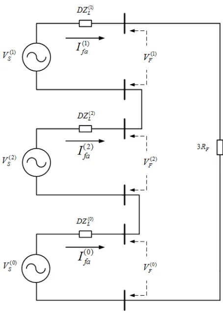
currents are equal during the fault. Using this implication, we must connect the positive, neg-ative and zero sequence networks in series as shown in Figure 2.10. The positive, negneg-ative and zero sequence impedance of the line are represented in the figure as ZL(1), ZL(2), and ZL(0)
respectively. The source voltage is also broken into sequence componentsVs(i).
Figure 2.9: Simple Feeder with no laterals or taps
To calculate the distance d to the fault, we begin with a simple KVL loop around the positive, negative and zero sequence parts of Figure 2.10 to solve for sequence voltage at the fault:
Vf(1) =Vs(1)−DIf a(1)ZL(1) (2.60)
Vf(2) =Vs(2)−DIf a(2)ZL(2) (2.61)
Vf(0) =Vs(0)−DIf a(0)ZL(0) (2.62)
Vf(0)+Vf(1)+Vf(2)= 3If a(0)Rf (2.63) Summing equations 2.60, 2.61 and 2.62.
Vf(0)+Vf(1)+Vf(2)=hVs(0)+Vs(1)+Vs(2)i−DIf a(1)ZL(1)+If a(2)ZL(2)+If a(0)ZL(0) (2.64) We can substitute: Vf(0)+Vf(1)+Vf(2) =Vf and Vs(0)+Vs(1)+Vs(2) =Vs.
Vf =Vs−D
If a(1)ZL(1)+If a(2)ZL(2)+If a(0)ZL(0) (2.65)
The Girgis method assumes thatZL(2)=ZL(1).
Vf =Vs−D
Figure 2.10: Single line-to-ground fault sequence networks.
Rearranging yeilds:
Vf =Vs−DZ
(1)
L I
(1)
f a +I
(2)
f a +I
(0)
f a ZL(0) ZL(1)
!
(2.67)
Substituting If a−If a(0)=If a(1)+If a(2):
Vf =Vs−DZ
(1)
L If a−I
(0)
f a +I
(0)
f a ZL(0) ZL(1)
!
(2.68)
If we simplify:
Vf =Vs−DZL(1) If a+If a(0)
ZL(0)−ZL(1) ZL(1)
!
(2.69)
Vs=Vf +DZL(1) If a+If a(0)Z
(0)
L −Z
(1)
L
ZL(1)
!
(2.70)
Substituting Equation 2.63:
Vs= 3I
(0)
f aRf+DZ
(1)
L If a+I
(0)
f a
ZL(0)−ZL(1) ZL(1)
!
(2.71)
Let k= Z
(0)
L −Z
(1)
L
ZL(1)
Vs= 3If a(0)Rf +DZ
(1)
L
If a+I
(0)
f ak
(2.72)
Equation 2.72 can be divided by If a+If a(0)kwhich gives: Vs
If a+I
(0)
f ak
= 3I
(0)
f aRf
If a+I
(0)
f ak
+DZL(1) (2.73)
The above equation can be used to calculate the positive sequence reactance to the fault. This is accomplished by taking the imaginary part of both sides of Equation 2.73. Assuming
If and If a+If a(0)k are in phase, the imaginary part of 3I
(0)
f aRf
If a+I
(0)
f ak
would equal 0. This yeilds:
Im
Vs
If a+If a(0)k
=DX
(1)
L (2.74)
The above solution is called the positive sequence reactance method[9]. The obvious drawback of this solution is the assumption thatIf andIf a+If a(0)kare in phase. The Girgis method offers
a different solution which does not make this assumption.
To begin, we define the apparent impedance seen at the measurement bus as Zapp= Vs If a+I
(0)
f ak
.
Zapp=
3If a(0)Rf If a+I
(0)
f ak
+DZL(1) (2.75)
We then substitute Icomp = 3If a(0), where Icomp is the compensating current fed into the
fault.
Zapp=
IcompRf
If a+I
(0)
f ak
Next, the compensating current Icomp and the selected current If a+If a(0)kare broken into
real and imaginary parts:
Icomp =Id+jIq (2.77)
If a+If a(0)k=Is1+jIs2 (2.78)
The positive sequence impedance of the line, ZL(1) is broken into real and imaginary parts as well:
ZL(1)=R(1)L +jXL(1) (2.79) Substituting 2.77,2.78, and 2.79 into 2.76:
Zapp=D
R(1)L +jXL(1)+Rf(Id+jIq)
Is1+jIs2
(2.80)
In the above equation, the fault resistance and distance to the fault are unknown. To solve for the distance to the fault, the apparent impedance is broken in real and imaginary parts. This yields two equations and two unknowns.
Re(Zapp) =DR(1)L +Rf
IdIs1+IqIs2
Is21+Is22
| {z }
N
(2.81)
Im(Xapp) =DXL(1)+Rf IqIs1−IdIs2 I2
s1+Is22
| {z }
M
(2.82)
Substituting M and N for the terms above:
Re(Zapp) =DR(1)L +N Rf (2.83)
Im(Xapp) =DXL(1)+M Rf (2.84)
Solving for D:
D= RappM−XappN
R(1)L M−XL(1)N
(2.85)
2.3.3 Assessment of the Girgis Algorithm: Advantages and Disadvantages The Girgis algorithm is a very simple algorithm that can be easily implemented by a utility for basic fault locating. However, the method does have many negative attributes that make it an unacceptable choice for many modern utilities. The following conditions were not considered by the Girgis algorithm: non-homogenous lines, mutual coupling and system loading conditions.
System Loading
The Girgis algorithm considers the feeder to be unloaded at the time of the fault occurrence. This assumption causes large errors in heavily loaded feeders. In the event that the fault were to occur at the remote end of a long feeder, it is often the case that the current seen at the substation during the fault is not much greater than the load current. In this case, the load current presents a major issue resulting in degraded accuracy at the remote end of the network.
Non-Homogeneous Lines and Mutual Coupling
The direct determination of the distance to the fault assumes equal mutual coupling and self impedances of the line. In the event that the we have equal self impedance and unequal mutual impedance or visa-versa this results in coupling between sequence components1. In practice, equal self impedance and mutual coupling terms are rarely the case.
The Girgis algorithm also assumes the feeder conductors to be homogeneous. Many feeders are composed of many different types and sizes of conductor, resulting in a non-homogeneous system. This is a major disadvantage of this algorithm.
Localization of Multiple Fault Possibilities
The Girgis algorithm, much like many impedance based algorithms can return multiple fault possibilities. For example, if the fault is found to be 1 mile from the measurement point, there may be multiple locations that are 1 mile from the measurement point. The author does recognize this as a limitation and presents a excellent solution. When multiple fault locations are found, the operating characteristics of protective devices are used to eliminate possibilities. This will be discussed in a later chapter.
1
2.4
Fault Locating using Digital Fault Recorder Data(Saha
Al-gorithm)
2.4.1 Overview of Saha Method
The algorithm proposed by Mourari Saha uses fundamental voltages and current available at the substation before and after the fault[1]. The algorithm proposed by Saha can be broken into two major steps: calculation of the fault loop impedance and calculation of impedance along the feeder. By comparing the measured impedance with the calculated feeder impedance, an indication of the fault location can be obtained[1].
2.4.2 Fault Loop Impedance Determination
The algorithm suggested by Saha requires that the positive sequence fault loop impedance be calculated from the available voltages and currents at the substation. This impedance is later used to determine the faulty node in the network. To begin our analysis we consider a Phase-to-Phase fault involving phases B and C at some node in the network. A phase-to-phase fault is shown in Figure 2.11 at any arbitrary point in the distribution network. The parameters
If a, If b andIf c are the fault currents measured at the substation.
Assuming the system to be unloaded at the time of fault we can easily show that for a B-to-C fault thatIf c=−If band If a= 0. We can now transform the fault currents flowing in the
network into their respective symmetrical components using the transform in Equation 2.86.
If a(0) If a(1) If a(2)
= 1 3
1 1 1 1 α α2
1 α2 α
0
If b −If b
(2.86)
Reducing Equation 2.86 results in the following:
If a(1) =−If a(2) (2.87) The above equation forms the foundation of solving for the positive sequence fault loop impedance. Using Equation 2.87 we can form its circuit representation shown in Figure 2.12. If we preform a simple KVL loop on Figure 2.12, we obtain:
Vf a(1)−If a(1)Zkk(1)−ZfIf a(1)+If a(2)Zkk(2)−Vf a(2)= 0 (2.88)
system at some arbitrary busk is defined asZkk(1) and Zkk(2).
Figure 2.11: B-to-C Fault
Figure 2.12: Sequence Network Diagram for a Phase-to-Phase Fault.
Using Equation 2.87, we can eliminate all negative sequence currents:
Vf a(1)−If a(1)Zkk(1)−ZfIf a(1)−If a(1)Zkk(2)−Vf a(2)= 0 (2.89)
Vf a(1)−Vf a(2) If a(1)
=Zkk(1)+Zf +Zkk(2) (2.90)
We can break down Equation 2.90 in much simpler terms by analysing the numerator portion of the equation. The pre-fault measured voltages can be broken into their corresponding sequence components by using a equation similar to Equation 2.86:
Vaf Vbf Vcf =
1 1 1 1 α2 α
1 α α2
Vaf(0) Vaf(1) Vaf(2)
(2.91)
If we extract Vbf and Vcf we get the following equations:
Vbf =Vaf(0)+Vaf(1)α2+Vaf(2)α (2.92) Vcf =Vaf(0)+Vaf(1)α+Vaf(2)α2 (2.93) Subtracting Equation 2.92 from 2.93 yeilds:
Vbf−Vcf =Vaf(1) α2−α
+Vaf(2) α−α2
(2.94)
Substituting α= 16 120◦:
Vbf −Vcf =Vaf(1)
−√3j)+Vaf(2)√3j) (2.95) We can now solve for Vaf(2)−Vaf(1):
Vaf(2)−Vaf(1)= Vbf√−Vcf
3j (2.96)
If we substitute 2.96 into 2.90 we get:
Vbf√−Vcf
3j If a(1)
=Zkk(1)+Zf +Zkk(2) (2.97)
Using a the symmetrical component transform similar to Equation 2.86, we can show that the positive sequence fault current yields:
If a(1)= 1
3 αIf b−α
2I
f b
Reducing yields:
If a(1) =
√
3
3 jIf b (2.99)
Substituting Equation 2.99 into Equation 2.97:
Vbf√−Vcf
3j
√
3 3 jIf b
=Zkk(1)+Zf +Zkk(2) (2.100)
Reducing Equation 2.100 yields:
Vbf−Vcf If b
=Zkk(1)+Zf +Zkk(2) (2.101) If we assume that the positive and negative sequence impedances are equal Zkk(1) =Zkk(2):
Vbf−Vcf If b
= 2Zkk(1)+Zf (2.102)
During fault conditions 2If b=Ibf−Icf:
Vbf−Vcf Ibf−Icf =Z
(1)
kk +Zf (2.103)
Assuming the fault to be bolted Zf = 0:
Vbf −Vcf Ibf −Icf =Z
(1)
kk (2.104)
The above equation represents the positive sequence impedance to the fault. We can use the available voltages Vbf and Vcf and currents If b and If c to calculate the positive sequence
fault loop impedance. However, with the fault resistance being unknown, we must assume that the fault is bolted Zf = 0.
2.4.3 Determination of the Faulty Node
Figure 2.13: Simple Substation with Two Parallel Feeders during Pre-Fault Conditions.
During the pre-fault conditions, we can define the pre-fault positive sequence impedance seen by the fault locator asZpre(1). This is represented in equation form as:
Zpre(1) = Z
(1)
k Z
(1)
lk
Zk(1)+Zlk(1)
(2.105)
During fault conditions, as shown in Figure 2.14, we represent the positive sequence impedance seen by the fault locator as:
Zf(1)= Vb−Vc
Ib−Ic
= Z
(1)
f kZ
(1)
lk
Zf k(1)+Zlk(1)
(2.106)
Our objective is to calculate the positive sequence loop impedance of the faulty feederZf k(1). Solving Equation 2.106 forZf k(1) we get:
Zf k(1) = Z
(1)
f Z
(1)
lk
Zlk(1)−Zf(1)
(2.107)
If we solve Equation 2.105 forZlk(1) we get:
Zlk(1)= Z
(1)
preZk(1) Zk(1)−Zpre(1)
Figure 2.14: Simple Substation with Two Parallel Feeders during Fault conditions.
Substituting Equation 2.108 into Equation 2.107:
Zf k(1)= Z
(1)
k Z
(1)
pre
Zpre(1)−Zf(1)
Zk(1)−Zpre(1) Zk(1)
!
| {z }
kzk
(2.109)
Consequently, kzk can also be related to Zpre(1) andZlk(1): kzk =
Zpre(1) Zlk(1)
(2.110)
Substituting:
Zf k(1)= Z
(1)
k Z
(1)
pre
Zpre(1)−Zf(1)Z
(1)
pre
Zlk(1)
(2.111)
Zf k(1) = Z
(1)
k Z
(1)
pre
Zpre(1) −Zf(1)kzk
(2.112)
Zf(1)= Va−Vb
Ia−Ib
= Vφ−φ
Iφ−φ
(2.113)
If we substitute Equation 2.113 into 2.117:
Zf k(1)= Vφ−φ
Iφ−φ−kzk Vφ−φ
Zpre(1)
(2.114)
The above equation represents the positive sequence loop impedance of the faulty feeder during fault conditions. It is assumed that the impedance of the adjacent parallel feeders do not change during fault conditions(this may not always be the case).
Now that the positive sequence loop impedance of the faulty feeder has been calculated, we can begin to search for the faulty line. The algorithm suggested by Saha sweeps the network for the faulty node until a specific set of criterion exists. One the criterion has been met, the faulty line section is found.
Figure 2.15: Cascaded Line Sections of Distribution Feeder.
We will begin our search for the faulty node at some nodei−1 in the network. We will represent the impedance of the cable between i−1 and i by Zsi(1)−1. The load at the remote node i is represented by Zpi(1). By using network reduction, we can develop a relationship between the impedance seen looking into the system at i−1 and i(Which isZf i(1) and Zf i(1)−1 respectively).
Zf i(1)−1 = Z
(1)
f i Z
(1)
pi
Zf i(1)+Zpi(1) +Z
(1)
si−1 (2.115)
Zf i(1)=
Zpi(1)Zf i(1)−1−Zsi(1)−1 Zpi(1)−Zf i(1)−1+Zsi(1)−1
(2.116)
Let us assume the substation bus to be i−1; assuming the load impedances to be known, we can now traverse each line section and calculate the impedance seen looking into the system from the remote bus. As expected |Zf i(1)|<|Zf i(1)−1| as we approach the faulty line. If we were traverse down the feeder and the value of Im(Zf i(1)) would be become less than zero, we would know the fault exists between i−1 andi.
To begin our search for our faulty line section, we always begin at the substation and work outwards. In this particaluar scenario, the substation may representi−1. As we move outward on the feeder, the value of Im(Zf i(1)) decreases. When the value of Im(Zf i(1)) becomes negative, the faulty line section has been found[32]. This part of the algorithm only identifies that the line section between i−1 and iis faulty. The distance from i−1 to the fault will be covered in the next section.
2.4.4 Distance to the Fault
After we have identified the fault line section(iand i−1) we must now determine the distance from node i−1 to the fault(distance down the line to the fault). Using a change in notation, we will call the faulted linek andk+ 1 in the following example(k=i−1 andk+ 1 =i).
Figure 2.16: Faulted Distribution Feeder[1].
Let us begin by assuming that the positive sequence loop impedance from node 1 tok, Z1(1)k
is known from pre-calculated tabulated values. Also, we will assume that the impedance of the shunt load at node 2 Zl(1)2 is also known. Any impedance beyond node kis lumped together as a shunt impedance called ∆Zf(1). The circuit representation of the faulty network seen by the fault locator is represented by Figure 2.17.
Figure 2.17: Circuit Representation of Network for a Fault located between 1 andk.
We will begin our derivation by assuming that the impedance seen by the fault locator is defined asZ1(1)f.
Z1(1)f = Vφ−φ
Iφ−φ
(2.117)
In the above figure, the variablem is used as a percentile over the total length of the cable from node 1 to node k. In this example the load is 1−m distance from the measurement point and m from the origination terminal of the faulted line section(node k). The equation representation of impedance seen by the fault locator described by Figure 2.17:
Z1(1)f = Vφ−φ
Iφ−φ
=
mZ1(1)k + ∆Zf(1)Zl(1)2 mZ1(1)k + ∆Zf(1)+Zl(1)2
∆Zf(1) =
Z1(1)k −Z1(1)f mZ1(1)k +Zl(1)2 −mZ1(1)k2 mZ1(1)k −Zl(1)2 −Z1(1)k −Z1(1)f
(2.119)
Previously we defined ∆Zf(1)as the lumped impedance representative of all elements beyond
k. In order to solve for the distance to the fault from k, we must define ∆Zf(1) in much more detail.
We can represent ∆Zf(1) as the circuit shown in Figure 2.18. All elements beyond node k
are represented, including the fault resistance. In Figure 2.18, xrepresents the distance to the fault from node k and ZL(1) represents the positive sequence impedance of the line from node
k to k+ 1. Also since a shunt load is present at node k, this is represented by Zlk(1). We also must represent all elements beyond node k+ 1; this positive sequence thevanin impedance is represented by Zk(1)+1.
Figure 2.18: Circuit Representation of Network for a Fault located betweenk and k+ 1.
Using network reduction we can reduce Figure 2.18 to the following equation:
∆Zf(1)=
Zlk(1) xZL(1)+Rf
(1−x)ZL(1)+Zk(1)+1 Rf+(1−x)ZL(1)+Z
(1)
k+1
!
Zlk(1)+xZL(1)+ Rf
(1−x)ZL(1)+Zk(1)+1
Rf+(1−x)Z
(1)
L +Z
(1)
k+1
![Figure 2.2: Flow Chart for Determining fault type[25].](https://thumb-us.123doks.com/thumbv2/123dok_us/1579060.1194349/22.612.163.458.77.350/figure-flow-chart-for-determining-fault-type.webp)

![Figure 2.4: Radial Distribution Feeder[25].](https://thumb-us.123doks.com/thumbv2/123dok_us/1579060.1194349/24.612.179.450.533.605/figure-radial-distribution-feeder.webp)


![Figure 2.16: Faulted Distribution Feeder[1].](https://thumb-us.123doks.com/thumbv2/123dok_us/1579060.1194349/48.612.237.391.439.595/figure-faulted-distribution-feeder.webp)