DOI: 10.1534/genetics.108.098129
Approximate Bayesian Computation Without Summary Statistics:
The Case of Admixture
Vitor C. Sousa,*
,†,1Marielle Fritz,
‡Mark A. Beaumont
§and Loune`s Chikhi*
,**
*Instituto Gulbenkian de Cieˆncia, Rua da Quinta Grande, P-2780-156 Oeiras, Portugal,†Centro de Biologia Ambiental, Faculdade de Cieˆncias da Universidade de Lisboa, Campo Grande, 1749-016 Lisboa, Portugal,‡Laboratoire de Statistiques et Probabilite´s, UMR C5583
Universite´ Paul Sabatier, 31062 Toulouse Ce´dex 09, France,§University of Reading, Whiteknights, RG6 6BX Reading, United Kingdom and**Laboratoire Evolution et Diversite´ Biologique, UMR CNRS/UPS 5174
Universite´ Paul Sabatier, 31062 Toulouse Ce´dex 09, France Manuscript received October 31, 2008 Accepted for publication January 21, 2009
ABSTRACT
In recent years approximate Bayesian computation (ABC) methods have become popular in population genetics as an alternative to full-likelihood methods to make inferences under complex demographic models. Most ABC methods rely on the choice of a set of summary statistics to extract information from the data. In this article we tested the use of the full allelic distribution directly in an ABC framework. Although the ABC techniques are becoming more widely used, there is still uncertainty over how they perform in comparison with full-likelihood methods. We thus conducted a simulation study and provide a detailed examination of ABC in comparison with full likelihood in the case of a model of admixture. This model assumes that two parental populations mixed at a certain time in the past, creating a hybrid population, and that the three populations then evolve under pure drift. Several aspects of ABC methodology were investigated, such as the effect of the distance metric chosen to measure the similarity between simulated and observed data sets. Results show that in general ABC provides good approximations to the posterior distributions obtained with the full-likelihood method. This suggests that it is possible to apply ABC using allele frequencies to make inferences in cases where it is difficult to select a set of suitable summary statistics and when the complexity of the model or the size of the data set makes it computationally prohibitive to use full-likelihood methods.
T
HE genetic patterns observed today in most species are the result of complex histories, which include demographic events such as population admixture, expansions, and/or collapses. The detection and quan-tification of such events relies on the fact that different scenarios leave a specific genetic signature in present-day populations, as well as on knowledge from other sources (e.g.ecology, biogeography, archeology) to define plau-sible models to explain such patterns. Recent population genetic modeling has seen the development of a number of statistical approaches that aim at extracting as much information as possible from the full allelic distributions (Griffiths and Tavare´ 1994; Wilson and Balding 1998; Beaumont1999; Beerliand Felsenstein2001; Chikhiet al.2001; Storzet al. 2002). These approaches aim at computing the likelihoodL(u),i.e., the probabilityPM(Dju) of generating the observed dataDunder some demographic modelM, defined by a set of parameters
u¼(u1,. . .,uk). In Bayesian statistics, the posterior
den-sity is used to make inferences as it reflects the probability of the parameters given the data, and it is obtained
through the relationshipP(ujD)}L(u)P(u), whereP(u) summarizes prior knowledge (or lack thereof) regarding
ubefore the data are observed (Beaumontand Rannala 2004). For most demographic models there are no ex-plicit likelihood functions or the likelihood cannot be de-rived analytically. Therefore, full-likelihood approaches rely on methods that explore the parameter space ef-ficiently, such as importance sampling (IS) (Stephens and Donnelly 2000) and Markov chain Monte Carlo (MCMC) (Beerliand Felsenstein2001; Nielsenand Wakeley2001; Beaumont2003). However, these meth-ods are highly computer intensive, their implementation into complex and realistic models is difficult, and, at the moment, their applicability to analyze large data sets is reduced (Heyand Machado2003; Hey and Nielsen 2004). This has led to the development of methods that try to approximate the likelihood, such as approx-imate Bayesian computation (ABC) (Beaumont et al. 2002; Marjoram et al. 2003), composite likelihood (Hudson 2001; Nielsen et al. 2005), and product of approximate conditionals (PAC) (Liand Stephens2003; Cornuet and Beaumont 2007; Roychoudhury and Stephens2007).
The principle of ABC methods is to use simulations across a wide range of parameter values within a model
1Corresponding author:Instituto Gulbenkian de Cieˆncia, Rua da Quinta
Grande, No. 6, P-2780-156 Oeiras, Portugal. E-mail: [email protected]
to find the parameter values that generate data sets that match the observed data most closely (Beaumont
et al. 2002). In most studies, the allele frequency data are summarized by means of summary statistics (Fu and Li1997; Tavare´et al. 1997; WeissandvonHaeseler 1998; Pritchard et al. 1999; Tallmon et al. 2004; Thornton and Andolfatto 2006). ABC algorithms do not require an explicit likelihood function and are based on a rejection scheme to obtain an approximate sample from the joint posterior distribution. Briefly, this involves four steps: (i) simulation of data sets with different parameter values drawn from the prior distri-butions; (ii) computation of a set of summary statistics for each data set; (iii) comparison of the observed and simulated summary statistics using a distance metric,e.g., Euclidean distance; and (iv) rejection of the parameters that generated distant data sets. The posterior distribu-tion reflectsPM(ujd(Ss,So),d), whered(Ss,So) stands for the distance between the observed and the simulated summary statistics, anddis an arbitrary threshold. The choice ofd(and of the number of simulations) reflects to some extent a balance between computability and accuracy (Beaumontet al. 2002; Marjoramet al. 2003). In most ABC implementations the value ofd is set as a quantile (the tolerance level Pd) from the empirical
distance distribution found for a given observed data set, and typical values range from 105 to 102 (e.g., Estoup et al. 2004; Becquet and Przeworski 2007; Fagundes et al. 2007; Pascualet al. 2007; Bonhomme
et al. 2008; Cox et al. 2008). The quality of the ABC inference is expected to depend on the summary statistics, the distance metric, and the tolerance levelPd
used. As noted by some authors, one potential problem is that it may be difficult or even impossible to define a suit-able set of sufficient summary statistics (Marjoramet al. 2003).
Here, we show that it is possible to use the full allelic frequency distribution directly. The posterior distribu-tion is thus approximated byPM(ujd(Do,Ds),d), where
Do andDsstand for the observed and simulated allele frequency data, respectively. The advantage of this approach over the use of summary statistics is clear whend decreases toward zero and the number of sim-ulations increases to infinity, as the accepted points tend to the correct joint posterior distribution (Marjoram
et al. 2003). As suggested by Marjoram et al. (2003), a rejection scheme might be inefficient when the data are high dimensional, and it has so far been used by Plagnoland Tavare(2004) to infer the times of lineage split based on fossil records. In this study we show that an ABC algorithm using the allele frequencies can approx-imate the results of a full-likelihood method in a reasonably complex model involving three populations and admixture. Note that the allele frequencies can be viewed as summary statistics of the individual genotypes. From this perspective they are sufficient since they contain all the information of the genotypes from each
locus. We do not refer to this approach as based on summary statistics to avoid confusion with most ABC approaches, which usually use functions of the allele frequency distribution as summaries of the data.
We implemented this ABC approach for an admixture model identical to that of Chikhiet al. (2001) (Figure 1). These authors developed a MCMC approach based on the IS sampling scheme of Griffiths and Tavare´ (1994), which is implemented in the LEA software (Langella et al. 2001). Currently, LEA is the only Bayesian full-likelihood method based on allele frequen-cies available to estimate admixture proportions, and for ease of comparison we used the same model in the ABC framework. Note that there is another full-likelihood method to estimate admixture (Wang2003), but it is based on the maximization of the likelihood and hence comparisons are not straightforward (but see Excoffier
et al. 2005). For comparison purposes, we also developed an ABC algorithm using typical summary statistics (ABC_SUMSTAT). Our main interest was to explore the performance of the ABC using the full allele fre-quency distribution to determine whether it can provide reasonable estimates compared to the full-likelihood (LEA) and summary statistics-based approaches. To sum-marize, in this study we (i) propose and validate with simulated data a new ABC inference method using allele frequency data, (ii) compare these results with those ob-tained with a full-likelihood method (LEA) and a tradi-tional ABC method, and finally (iii) explore some general issues regarding the ABC approach, namely the choice of the distance metrics, the tolerance level, the number of simulations, and the use of a regression step.
MATERIALS AND METHODS
The admixture model:The model is represented in Figure 1. It assumes that two independent parental populations,P1 andP2, of sizeN1andN2, mixed some timeTin the past with respective proportionsp1andp2(¼1p1), creating a hybrid populationHof sizeNh. At the time of admixture, the gene frequency distributions ofP1and P2are represented by the two vectors x1 and x2, respectively, and that of the hybrid Figure1.—The admixture model described in the text. We
population by p1x1 1 p2x2. After admixture, P1, P2, and H evolve independently (with no migration) by pure drift (no mutations) until the present time. The time since admixtureT (in generations) is scaled by the effective size of each population, and the corresponding drift times are called t1¼T/N1,t2¼T/N2, andth¼T/Nh. This model is the same as in Thompson(1973). Flat priors were used for p
1, t1, t2, andth. The priors forx1 andx2were independent uniform Dirichlet distributions withkparametersD(1,. . ., 1), wherekis the number of alleles per locus observed across all present-day populations. These priors reflect independent parental pop-ulations with allele frequencies generated according to aK -allele mutation model withK¼k(Ewens 2004). Note that
Wang(2003) and Choisyet al. (2004) criticized this
admix-ture model because it ignores the correlation of the allele frequencies in the parental populations due to common ancestry. These authors propose alternative priors, but since they are not implemented in LEA, we kept the uniform Dirichlet in the ABC.
ABC without summary statistics (ABC_ALL_FREQ): The ABC using the allele frequencies is referred to as ABC_ALL_
FREQ. The rejection algorithm was divided into two parts as follows: (i) given a particular tolerance levelPdand a particular
data setDo, the corresponding toleranced* is obtained from the distance distribution of a first set of simulations (typically 104or 105); and (ii) a large number of simulations (.106) are then performed, keeping all parameter values for whichd(Do, Ds) ,d*. The division of the algorithm into two parts can reduce the computation time because there is no need to simulate the samples for all the loci and populations at each step of the second part. Whenever the distance after simulat-ing thej*th population from the l*th locus is higher than the tolerance (Pll*¼1
Pj*
j¼1dlj.d*), the parameter set is
rejected. In the first part, the tolerance was computed as the 0.1 or 0.001 quantiles of the distance distributions, obtained after 104or 105simulations for the single-locus and multilocus case, respectively. In the second part, 106 simulations were performed for the single-locus and 108for the multilocus case. The influence of the number of simulation steps was in-vestigated by repeating the analysis with 106, 107, and 108 simulations, for the multilocus case with 10 loci. The choice of the tolerance level was also investigated, looking at the results forPd-values between 105and 103.
Distance metrics (Euclidean and GST):Most studies to date use
a Euclidean distance. Here, two distance metrics were used to compute distances between simulated and observed data. For simplicity we focus on single-locus data from one population, which is represented by a vectorDo¼(o1,. . .,ok), whereoiis
the absolute frequency of allelei,i¼(1,. . .,k), andkis the total number of alleles observed across the three populations (i.e., someoican be zero in some populations, but not all). The
two distance measures used here were (i) a standardized Euclidean distance,deuc¼
ffiffiffiffiffiffiffiffiffiffiffiffiffiffiffiffiffiffiffiffiffiffiffiffiffiffiffiffiffiffiffiffiffiffiffiffiffiffiffi Pn
i¼1ððoisiÞ=oiÞ2
q
, whereoiandsiare
the absolute allele frequencies of the observed and simulated data sets, respectively, and (ii) the ‘‘genetic distance’’ GST, dGST¼1H=HT, where HT is the expected heterozygosity
(He) when the two vectorsDoandDsare pooled, andH is the averageHecomputed forDoandDs(Nei1986). The rationale
behind the use of theGSTdistance comes from the fact that we were using allele frequencies, not summary statistics. We refer to the first as Euclidean and the second asGST. The distance is computed for each population and locus independently, and the total distance was defined as the sum over loci and over populations, dT¼
P l
P
jdlj, where j ¼ 1, 2, hrefers to the
populations andl¼1,. . .,mto the loci.
As pointed out by Marjoram et al. (2003), using
high-dimensional data may reduce the acceptance rate and compromise the efficiency of the rejection algorithm.
How-ever, since all the loci share the same demographic history and mutation process (K-allele model),i.e., the loci and alleles are exchangeable under this admixture model, the full allelic distribution can be viewed as a highly dimensional unordered data set [as in label-switching problems (Stephens2000)]. In
these cases, due to exchangeability, the likelihood does not depend on the order of the elements. Therefore, it is possible to increase the acceptance rate using permutations of the allele and loci labels to minimize the total distance between observed and simulated data sets. These approaches are described below.
Sort the allele frequencies:Let us assume a single-population model in which we observe a single-locus data set with three alleles whose absolute frequencies are given by the vectorDo¼ (15, 5, 30) (hence a sample size of 25 diploids or 50 genes). Let us further assume that the following simulated data set is obtained:Ds¼(5, 30, 15). Given that the alleles are exchange-able, it is possible to permutate the allele labels and find an exact match between Ds and Do. In practice, the minimal distance was found by sorting the absolute allele frequencies. Since our model has three populationsP1,P2, andHand since the labels of alleles in the three populations are not in-dependent, the SORT algorithm sorts the alleles according to the allele frequencies of the three populations pooled together. We defined two algorithms referred to as SORT when alleles were sorted and as SIMPLE when the data sets are compared directly. We compared the SORT and SIMPLE algorithms in the single-locus case, using the Euclidean distance.
Reorder the loci:Consider a vector where each element con-tains the data of one locus, say Do ¼ (o1,. . .,ol) with l
ex-changeable loci,i.e., the order of the labels is irrelevant. When comparing this vector with a simulated one, sayDs¼(s1,. . .,sl),
there is a one-to-one correspondence but it is arbitrary to compareoiwithsi. Therefore, the labels of the loci were
per-muted to minimize the distance between the observed and the simulated data sets. The best solution requires the evaluation of alll! possible combinations, which may become impractical for the number of simulations performed here. Instead, we used a heuristic to approximate the minimal distance (but see Stephens2000 for a discussion on efficient algorithms applied
of this procedure in the estimates is dependent on the amount of missing data, and thus the analysis should be repeated with different resampled data sets to assess this effect. For the multilocus case we focused on unlinked biallelic markers. This choice was in part because of an increasing amount of data from genomic biallelic markers such as SNPs,e.g., HapMap (Frazeret al. 2007), RAPD, and RFLP (e.g., Parraet al. 1998),
and because in this case all loci have the same number of alleles. The performance of reordering the loci was compared with a procedure where the loci were compared randomly without minimizing the distance, by analyzing the data sets of 10 biallelic loci withti¼0.001 with the two approaches. Note
that a similar labeling problem was met by Rosenblumet al.
(2007), who used summary statistics and sorted the loci according to the values of one of the latter.
Regression step:Beaumontet al. (2002) showed that
perform-ing a weighted local linear regression on the parameters obtained during the rejection step improves the estimation results. The regression assumes that, at least locally, there is a linear relation between the mean value of the accepted parameters and the accepted summary statistics. In this case, the predictor variables were the allele frequencies (or sum-mary statistics for the ABC_SUMSTAT), and the response
variables were the parameters of interest (p1, t1, t2, th). However, as can happen with some summary statistics, the relation between the allele frequencies and the parameters of interest is not necessarily linear. Forp1the linear assumption appears to be valid, as the allele frequencies among popula-tions are linearly correlated withp1, at least immediately after the admixture event. However, fort1,t2, andththe mean value of the parameters does not change according to a linear relation with the allele frequencies. In a stable population there is a positive relation between the variance of the allelic frequency and drift. We thus performed two different regres-sions, (i) independent regression, applied for p1, and (ii) multiresponse quadratic regression, applied tot1,t2,th. In the first, due to the fact that within each locus in a population the allele frequencies are correlated (i.e., the sum is one), the regression was performed discarding the most frequent allele across populations from each locus. In the second, the allele frequencies were squared and thet1, t2,th were considered altogether in a single linear model, using dummy variables to code each parameter (Neteret al. 1985). The linear model
becomesY ¼b01Pn
j¼1bjXj21bd1D11bd2D21e, wheren¼
na3l(naalleles andlloci), andeis the error.Yis a vector with the m accepted parameters pooled together, Y ¼ (t1*1,. . .,t1*m, t2*1,. . .,t2*m, th*1,. . .,th*m). Each Xj is a vector
with the correspondingmaccepted squared allele frequencies Xj¼(xj*1,. . .,xj*m,xj*1,. . .,xj*m,xj*1,. . .,xj*m), wherexj*iis the
allele frequency of thejth allele in theith accepted simulation. TheDdummy variables are coded with values 0 or 1 to identify each parameter. To estimatet1the two dummy variables are equal to 0 and the model becomes E½t1 ¼b01Pn
j¼1 bjXj21e. To estimatet2,D1¼1 andD2¼0, and the model becomesE½t2 ¼b01Pn
j¼1bjXj21bd11e. Finally, to estimate
t3 the two dummy variables are equal to 1, and the model becomesE½t3 ¼b01Pn
j¼1bjXj21bd11bd21e. The estimated
bd1andbd2reflect the difference in the intercept of the threeti
parameters. In both regressions, the accepted parameters were weighted according to the corresponding distances using the Epanechnikov kernel, as in Beaumontet al. (2002). The
parameters were transformed to avoid posterior values outside the prior distribution limits, following the transformation of Hamiltonet al. (2005).
ABC with summary statistics (ABC_SUMSTAT): To de-termine whether our ABC approach was comparable to a summary statistics-based approach we also developed an ABC algorithm with 14 summary statistics, which is referred to as
ABC_SUMSTAT. The summary statistics were chosen on the
basis that they should contain information about the param-eters of interest in the admixture model. Namely, we used (i) the expected heterozygosity (He) for each population and over all populations, (ii) the number of alleles na of each population, (iii) the number of private alleles np of each population, and (iv) the three pairwiseFSTand the overallFST. As in Beaumontet al. (2002), the distance metric considered
was a Euclidean distance between the standardized observed and simulated summary statistics,d¼ ffiffiffiffiffiffiffiffiffiffiffiffiffiffiffiffiffiffiffiffiffiffiffiffiffiffiffiffiffiffiffiffiPððSoiSsiÞÞ
2
q
,i¼1,. . .,s wheresis the number of summary statistics. For the multilocus case, we used the mean of each summary statistic across loci. The summary statistics were standardized by subtracting the mean and dividing by the standard deviation of the simu-lations performed in the first part of the rejection algorithm, 104 for the single locus and 105 for the multilocus. The rejection step was done with the same number of simulation steps and the same tolerance values as for ABC_ALL_FREQ. A
local weighted regression between the standardized summary statistics and the accepted parameters was performed as in Beaumontet al. (2002), transforming the parameters as in
Hamiltonet al. (2005).
Data simulation:The data sets used to test the performance of the different methods were simulated for each locus according to the demographic model depicted in Figure 1, using the coalescent. More specifically, the simulation algo-rithm was as follows:
i. Sample parameters p1*, t1*, t2*, and th* from the prior distributions.
ii. Sample the ancestral allele frequenciesx1* andx2* from a uniform DirichletD(1,. . ., 1). The allele frequency of pop-ulationHat the time of admixture is set toxh*¼p1*3x1*1 (1p1*)3x2*.
iii. Sample the coalescent times, for each population in-dependently, from an exponential distribution until the admixture event at time ti*, where i¼ 1, 2,h. At each
coalescent event the number of lineages decreases by one. The lineages that remain at timeti* are designated as
founder lineages.
iv. Sample the allelic state of the founders from the ancestral allele frequenciesx1*,x2*,xh*.
v. Starting from the founder lineages to the present-day samples, lineages are randomly picked and duplicated for every coalescent event, until the present-day sample size is reached (Beaumont2003).
This algorithm was used in the two ABC approaches and to generate all the data sets analyzed. Samples from 108 simu-lations with 10 independent biallelic loci were saved in a database, and this was used to perform the rejection step, in the multilocus case, for all the ABC approaches.
Comparison of approximate (ABC) and full-likelihood (LEA) methods: The relative performance of the different approaches (see Table 1), including the full-likelihood method, was evaluated with samples generated with the following set of parameter values. Two different levels of drift, namelyti¼0.001 andti¼0.01, (i¼1, 2,h), were used,
assuming that the three populations evolved under the same conditions (i.e., t1 ¼ t2 ¼ t3). For each level of drift, we simulated 50 gene copies (25 diploid individuals) typed at 1, 5, and 10 unlinked loci, with an admixture proportionp1¼ 0.7. For the single-locus data sets, we simulated loci with 2, 5, and 10 alleles. For multilocus loci, only biallelic markers were simulated. For each combination of parameters we simulated 50 independent data sets. These simulated data sets were then given as input to LEA, ABC_SUMSTAT, and ABC_
For LEA we ran one MCMC chain for each generated sample with 105steps and a thinning interval of 5 as suggested in Chikhi et al. (2001). At each step, the likelihood was
estimated with 500 iterations of the importance sampler. The density estimation of the posterior distribution was performed discarding the first 10% of the chain (burn-in). For the 10-locus case, we conducted convergence analysis by comparing the results obtained with longer runs (106steps) and found no difference. Thus, 105steps were used in all the analyses, as LEA was clearly the slowest of the methods tested. The only difference between the full-likelihood and the approximate methods is in the priors for theti’s. LEA assumes uniform but
improper priors (with no upper bound). In the ABC, the priors are also uniform but we defined an upper bound at 0.2, since the data sets were all generated with much smaller ti
values. Of course, for the analysis of real data sets, for which theti’s are unknown, higher bounds can be allowed.
Neverthe-less, to avoid any bias in the comparison, we conditioned the sample from the posterior obtained with LEA such thatti#
0.2, and the posterior of interest is thusPM(p1,t1,t2,thjD,ti#
0.2). The different methods were compared by looking at properties of the full posterior distributions and at point estimates. We measured (i) the mean integrated square error (MISE) of each data set, which reflects the posterior density around the real parameter value (ð1=nÞPn
i¼1ðuiuÞ
2 =u2), wherenis the number of accepted points used to obtain the posterior, and (ii) the relative root mean square error (RRMSE) of the median, which is the square root of the mean square error divided by the true valueðð1=uÞ ffiffiffiffiffiffiffiffiffiffiffiffiffiffiffiffiffiffiffiffiffiffiffiffiffiffiffiffiffiPðuiuÞ
2 =n
q
Þ, where nis the total number of data sets analyzed. The confidence intervals for the RRMSE of each parameter were obtained with a nonparametric bootstrap, using 1000 iterations. Note that the RRMSE was computed as the mean of 50 independent data set analyses, and thus it should be considered indicative and not an absolute estimate of the error. In total, we simulated 500 different data sets that were analyzed by all the different methods, for a total of 2100 analyses (excluding the regression step results). The programs are available upon request. The rejection step for the three ABC programs was written in C. The regression analysis was performed in R using the lm function (R Development Core Team 2008). The locfit
function implemented in R was used to estimate the density of the marginal posteriors (Loader2007).
Analysis of a human data set:We applied the ABC methods to a data set published by Parraet al. (1998) and previously
analyzed with LEA by Chikhiet al. (2001). The original data
set consists of nine nuclear loci (restriction site and Alu polymorphisms) typed in populations from Europe, Africa, the United States (African-Americans from different cities),
and Jamaica. The aim was to estimate the admixture pro-portions in African-Americans and in Jamaica, using the European and African data as parentals. Most loci were biallelic with the exception of one locus that was triallelic. We focused on the Jamaican sample (averagen¼185.8) as the hybrid (H) and considered that the samples from parental populationsP1andP2correspond to all the samples pooled together from Europe (averagen¼292.4) and Africa (average n¼387.6), respectively. The allele frequencies are the same as in Table 3 of Chikhi et al. (2001). Two approaches of the
ABC_ALL_FREQ were used since the data set had loci with
different numbers of alleles and different sample sizes. In the first, the original data set was used and no permutations were performed to minimize the distance between the observed and the simulated data sets. In the second, we created a resampled data set by sampling the allele frequencies until all loci had the same sample size at each population. This allowed us to use permutations to find the minimal distance between the simulated and the observed data set. The original data set and the resampled data set were analyzed with all the methods. Forp1, a flat prior between zero and one was assumed. For the ti’s, three different flat priors were tested, varying the upper
limit as 0.2, 0.5, or 1. For the three ABC approaches we per-formed 107simulations in the rejection step with a tolerance level of 0.1% (Pd¼0.001), and the regression step was applied
as in the simulation study. The effect of resampling was assessed repeating the analysis with 10 different resampled data sets using ABC_ALL_FREQ withG
STdistance. For LEA, three independent MCMC runs were performed with 106steps each.
RESULTS
Simulation study: The posterior distributions ob-tained for the single-locus case with the ABC and full-likelihood methods are compared in Figure 2, for three representative runs with different numbers of alleles and a tolerance levelPd¼0.001 (1000 simulation data
sets accepted out of 106simulations). Figure 2, together with the associated Table 2, shows that full-likelihood and ABC methods produce similar results. As expected, increasing the number of alleles leads to narrower poste-riors around the true parameter values. For all methods, thep1RRMSE decreases when drift decreased and when the number of alleles increased from two to five (Table 2). Thus, betterp1estimates were obtained when drift was TABLE 1
Summary of different methods compared
Approximate (ABC)
ABC_ALL_FREQ Full likelihood
(LEA) GST Euclidean ABC_SUMSTAT
Data in P(ujD)
All. freq. All. freq. All. freq. Summary statistics
Distance metric
— GST(Nei1986) Standardized
Euclidean
Euclidean
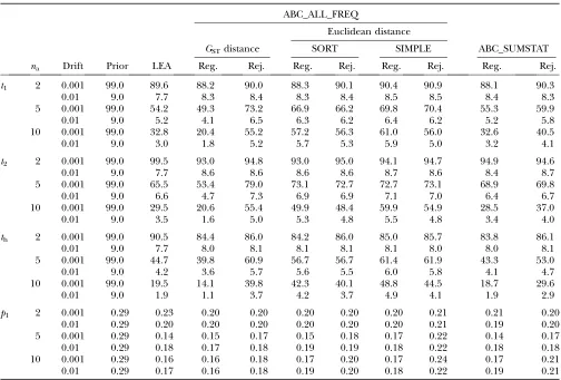
limited and when the locus had a higher number of alleles, as described previously (Chikhiet al. 2001; Wang 2003; Excoffieret al. 2005). The RRMSE ratio of each ABC method over LEA ranged from 0.99 to 1.36, showing that some ABC methods have near-identical RRMSE values to LEA. Among the ABC methods, smaller errors were obtained with ABC_ALL_FREQ using the GST distance. The MISE results showed a slightly different pattern, with LEA exhibiting increasingly better results as the number of alleles increased (supplemental Table 1). Theti’s RRMSE also decreased with increasing numbers of alleles. In most repetitions the posteriors of theti’s had a mode close to zero, as seen in the examples in Figure 2, but a median close to 0.1, which is also the median of the prior, confirming that the ti’s are difficult to estimate (Chikhiet al. 2001; Wang2003). In general,thexhibited the smallest RRMSE whereast2exhibited the largest error values. This is probably due to the fact thatP2contributed less to the hybrid population and hence provided less genetic information (Wang 2003). An apparently sur-prising result was that in most cases the RRMSE was slightly larger for LEA than for the ABC methods (ABC_ALL_FREQGSTand ABC_SUMSTAT). However, the RRMSE confidence intervals overlapped consider-ably, suggesting no significant differences among meth-ods. Regarding the relative performance of sorting the alleles,i.e., SIMPLEvs.SORT, the latter exhibited lower RRMSE and MISE values and no bias, with both the rejection and the regression steps (Table 2). Thus, for the multilocus case we considered only the SORT approach.
Multilocus data: The posterior distributions obtained with the approximate and full-likelihood methods for the multilocus data are represented in Figure 3, for the
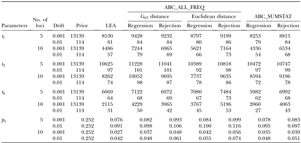
p1 parameter. As with single-locus data, the different methods produced similar distributions. Increasing the number of loci produced more accurate and precise distributions, reducing the RRMSE and MISE (Tables 3 and 4). Forp1, the ABC point estimates were close to the ones obtained with LEA, producing nearly identical RRMSE values (Table 3). Note that in some cases the RRMSE was slightly smaller with the rejection step of ABC methods. For instance, the RRMSE ratio for p1 varied between 0.99 and 1.02 for the rejection step of ABC_ALL_FREQ with the GST distance and between 0.98 and 1.06 for ABC_SUMSTAT. However, the ABC posteriors tended to be wider than the full likelihood, as reflected by the higher MISE for the ABC methods (Table 4). LEA provided the posterior distributions with the smallest MISE, but ABC_SUMSTAT and ABC_ALL_ FREQ with GST approximated reasonably well those values with the regression step. Note that the difference between the full likelihood and the ABC was typically higher with 10 loci, suggesting that LEA is better at using additional information brought by new loci. For theti’s, the smallest average MISE was obtained with LEA and ABC_SUMSTAT. Focusing on the ABC_ALL_FREQ, the
GST distance metric tends to provide estimates with a smaller error than the Euclidean. Also, reordering the loci minimizing the distance of each simulation led to posteriors with higher density close to the true param-eter values and closer to the ones obtained with the full likelihood.
Effect of tolerance, regression, and number of simulation steps: The three ABC methods had the same behavior when the tolerance level varied, with lower RRMSE and MISE values when the tolerance level decreased (Figure Figure2.—Example of posterior distributions
4). Although the ABC rejection step reached RRMSE values similar to LEA forp1, the MISE did not approach the values of the full-likelihood method. The perfor-mance of the ABC methods approached LEA’s only when the regression step was performed, and in this case the error decreased significantly over the rejection step even for the highest tolerance levels considered here. For the drift parameters, the situation was slightly different for the ABC_ALL_FREQ methods, since the regression did not lead to major improvements over the rejection. Note that the effect of the regression on the RRMSE was not clear forp1, as the RRMSE increased above that of the rejection step for the lower tolerance level. This was also observed by Beaumontet al. (2002), who suggested that it was potentially caused by the limited number of points used to perform the regres-sion (,500). However, this explanation may not apply here, since at least 1000 points were used and the MISE did not increase for the lower tolerance values. In-creasing the total number of simulations from 106to 108 does not lead to major differences, given the same tolerance level (Pd). As long as 1000 points were
accepted withPd¼103, the parameters were reasonably
well estimated after the regression step (not shown), suggesting that 1 million simulations were enough to get approximate results.
Human data set (admixture in Jamaica):As shown in Figure 5, the posteriors forp1obtained with LEA had a high density around 0.07 (0.025–0.124), suggesting a limited contribution of Europeans to the Jamaican gene pool. The 0.05 and 0.95 quantiles of the posteriors are shown inside parentheses. For t1 the posteriors had higher density around 0.2 (0.07–0.61). However, the posteriors were similar to the priors, suggesting limited information about t1. Fort2andththe posteriors were clearly different from the priors and supported drift values close to zero (0.0016–0.0734 fort2and 0.0004– 0.0412 forth). As discussed by Chikhiet al. (2001), this is suggestive of a recent admixture event.
The ABC methods returned point estimates for p1 similar to LEA, although the posteriors were less precise (0.013–0.320 for GST, 0.015–0.235 for Euclidean, and 0.009–0.260 for ABC_SUMSTAT). ABC_ALL_FREQ produced the posterior closest to the full-likelihood results. For the ti’s, the ABC posteriors were very wide and approached LEA’s results only qualitatively;i.e., they TABLE 2
Relative root mean square error (RRMSE) for single-locus analysis
ABC_ALL_FREQ
Euclidean distance
GSTdistance SORT SIMPLE ABC_SUMSTAT
na Drift Prior LEA Reg. Rej. Reg. Rej. Reg. Rej. Reg. Rej.
t1 2 0.001 99.0 89.6 88.2 90.0 88.3 90.1 90.4 90.9 88.1 90.3
0.01 9.0 7.7 8.3 8.4 8.3 8.4 8.5 8.5 8.4 8.3
5 0.001 99.0 54.2 49.3 73.2 66.9 66.2 69.8 70.4 55.3 59.9
0.01 9.0 5.2 4.1 6.5 6.3 6.2 6.4 6.2 5.2 5.8
10 0.001 99.0 32.8 20.4 55.2 57.2 56.3 61.0 56.0 32.6 40.5
0.01 9.0 3.0 1.8 5.2 5.7 5.3 5.9 5.0 3.2 4.1
t2 2 0.001 99.0 99.5 93.0 94.8 93.0 95.0 94.1 94.7 94.9 94.6
0.01 9.0 7.7 8.6 8.6 8.6 8.6 8.7 8.6 8.4 8.7
5 0.001 99.0 65.5 53.4 79.0 73.1 72.7 72.7 73.1 68.9 69.8
0.01 9.0 6.6 4.7 7.3 6.9 6.9 7.1 7.0 6.4 6.7
10 0.001 99.0 29.5 20.6 55.4 49.9 48.4 59.9 54.9 28.5 37.0
0.01 9.0 3.5 1.6 5.0 5.3 4.8 5.5 4.8 3.4 4.0
th 2 0.001 99.0 90.5 84.4 86.0 84.2 86.0 85.0 85.7 83.8 86.1
0.01 9.0 7.7 8.0 8.1 8.1 8.1 8.1 8.0 8.0 8.1
5 0.001 99.0 44.7 39.8 60.9 56.7 56.7 61.4 61.9 43.3 53.0
0.01 9.0 4.2 3.6 5.7 5.6 5.5 6.0 5.8 4.1 4.7
10 0.001 99.0 19.5 14.1 39.8 42.3 40.1 48.8 44.5 18.7 29.6
0.01 9.0 1.9 1.1 3.7 4.2 3.7 4.9 4.1 1.9 2.9
p1 2 0.001 0.29 0.23 0.20 0.20 0.20 0.20 0.20 0.21 0.21 0.20 0.01 0.29 0.20 0.20 0.20 0.20 0.20 0.20 0.21 0.19 0.20
5 0.001 0.29 0.14 0.15 0.17 0.15 0.18 0.17 0.22 0.14 0.17
0.01 0.29 0.18 0.17 0.18 0.19 0.19 0.18 0.22 0.18 0.18 10 0.001 0.29 0.16 0.16 0.18 0.17 0.20 0.17 0.24 0.17 0.21 0.01 0.29 0.17 0.16 0.18 0.19 0.20 0.18 0.22 0.19 0.21
ABC results obtained with 106simulations are shown, accepting the closest 1000 (P
d¼103).na, number of alleles; Reg.,
pointed to higher drift in Europe, limited drift in Africa, and even less drift in Jamaica. For theti’s, ABC_SUM STAT returned estimates closer to LEA than ABC_ALL_ FREQ. The analysis of the resampled data set lead to identical results with LEA’s, and almost no differences were found with the ABC methods after the regression step. As expected, for ABC_ALL_FREQ, the rejection step performed better with the resampled data set. The analysis of different resampled data sets returned similar posteriors, suggesting that the effect of resam-pling was limited in this case (supplemental Figure 1). On the contrary, reanalyzing the data sets varying the upper limit for thetipriors affected significantly thep1 posteriors. Better estimates were obtained with lower upper limits (Figure 6). The reason is that the trueti
values are more likely close to zero, and hence reducing the upper limit of thetiprior led the ABC methods to explore more often the most likely parameter space.
DISCUSSION
Altogether our simulations and the real data set analysis show that the ABC using the full allelic distri-bution (ABC_ALL_FREQ) can be used to estimate
parameters under a relatively complex demographic model. The results obtained here were similar to those obtained using summary statistics (ABC_SUMSTAT) and were comparable to those obtained with a full-likelihood method also based on allele frequency data. The ABC methods produced broader posterior distri-butions but did not appear to be biased (Tables 3 and 4). In principle, by increasing the number of simulations to infinity (or a very large number) the ABC based on allele frequency should produce results identical to LEA, while this would not necessarily be the case with the summary statistics due to the inevitable loss of informa-tion when summarizing the data (Marjoramet al. 2003). In practice, and given the number of simulations performed (between 106 and 108), LEA tended to produce better results than the ABC algorithms, al-though it was at least 10 times slower as the number of loci increased.
Focusing on the rejection step, the two ABC ap-proaches (ABC_ALL_FREQ and ABC_SUMSTAT) gen-erated posterior distributions with point estimates close to the true value and similar to LEA. However, with 10 loci, even when the number of simulations increased up to 108and the tolerance levelP
dwas lowered to 105, the
Figure3.—Comparison of the posterior distributions obtained forp1with the different methods for the multiple biallelic loci
case, with driftti¼0.01. The results obtained with 5 and 10 loci are shown in the top and bottom rows, respectively. Each solid line
corresponds to the posterior obtained for 1 of the 50 repetitions. For the ABC methods, the densities were obtained with the regression step. The prior distributions are shown as dotted horizontal lines and the true parameter values as dashed vertical lines. ABC results obtained with 108simulations andP
posteriors were still wider than with LEA (Table 4). These results confirm the relatively poor efficiency of the rejection scheme when dealing with large data sets. This is potentially more problematic for the ABC_ALL_ FREQ scheme, as the dimensionality increases quickly with the size of the data sets. Several approaches were tested here to minimize this problem by (i) sorting the
allele frequencies, (ii) reordering the loci, and (iii) using different distance metrics, and all three improved the estimates.
A major improvement was observed forp1when the local weighted regression was applied leading to poste-riors close to LEA, even with 106 simulations (P
d ¼
0.001). For the ti’s, the regression step improved the
TABLE 4
Mean integrated square error (MISE) for multilocus analysis
ABC_ALL_FREQ
No. of loci
GSTdistance Euclidean distance ABC_SUMSTAT Parameters Drift Prior LEA Regression Rejection Regression Rejection Regression Rejection
t1 5 0.001 13139 8530 9428 9232 8797 9199 8253 8815
0.01 114 81 84 84 80 86 79 84
10 0.001 13139 4486 7244 6965 5621 7164 4336 6534
0.01 114 57 79 69 66 73 54 68
t2 5 0.001 13139 10625 11228 11041 10389 10818 10472 10747
0.01 114 97 101 101 92 98 97 99
10 0.001 13139 8262 10052 9695 7737 9635 8594 9196
0.01 114 74 98 87 78 86 72 78
th 5 0.001 13139 6069 7122 6972 7080 7484 5982 6992
0.01 114 64 68 69 67 73 62 68
10 0.001 13139 2115 4229 3965 3767 5196 2060 4063
0.01 114 31 50 42 45 53 27 43
p1 5 0.001 0.252 0.076 0.082 0.093 0.084 0.099 0.078 0.083
0.01 0.252 0.091 0.098 0.106 0.100 0.116 0.095 0.097 10 0.001 0.252 0.027 0.037 0.048 0.042 0.056 0.035 0.039 0.01 0.252 0.042 0.048 0.061 0.055 0.074 0.048 0.051
ABC results obtained with 108simulations are shown, accepting the closest 1000 (P
d¼105).
TABLE 3
Relative root mean square error (RRMSE) for the multilocus analysis
ABC_ALL_FREQ
No. of loci
GSTdistance Euclidean distance ABC_SUMSTAT Parameters Drift Prior LEA Regression Rejection Regression Rejection Regression Rejection
t1 5 0.001 99.00 66.46 73.40 70.39 67.89 70.80 64.24 68.65
0.01 9.00 6.60 6.72 6.67 6.45 6.97 6.33 6.75
10 0.001 99.00 42.43 61.58 54.69 49.43 59.36 40.44 56.44
0.01 9.00 5.16 6.83 5.57 5.90 6.25 4.72 5.89
t2 5 0.001 99.00 81.13 86.15 84.05 79.00 82.59 80.22 82.92
0.01 9.00 7.78 8.14 8.06 7.36 7.89 7.83 7.88
10 0.001 99.00 66.91 80.66 74.86 60.39 75.79 68.31 72.80
0.01 9.00 6.27 8.13 6.97 6.52 7.07 5.97 6.41
th 5 0.001 99.00 46.59 55.74 52.23 54.69 55.95 46.33 53.20
0.01 9.00 5.21 5.49 5.30 5.28 5.77 4.96 5.35
10 0.001 99.00 22.45 39.50 33.12 33.60 42.62 21.88 36.23
0.01 9.00 3.05 4.55 3.28 4.11 4.36 2.59 3.87
p1 5 0.001 0.286 0.119 0.118 0.122 0.116 0.129 0.112 0.118
0.01 0.286 0.157 0.158 0.155 0.162 0.171 0.159 0.155 10 0.001 0.286 0.067 0.078 0.067 0.081 0.079 0.072 0.071 0.01 0.286 0.109 0.114 0.111 0.119 0.124 0.113 0.107
ABC results obtained with 108simulations are shown, accepting the closest 1000 (P
posteriors of ABC_SUMSTAT but not of ABC_ALL_ FREQ. This is most likely because the allele frequency data do not fit properly the assumptions of the linear regression. Namely, it is not clear that the relation between allele frequency and drift is linear. In fact, better estimates were obtained assuming a linear re-lation between the time since admixture and the square of the allele frequencies, probably because it is the variance of allele frequencies that increases with drift. Drift affected significantly the estimation ofp1, and even with 10 biallelic loci the posteriors forp1 were rather wide withti ¼0.01 (10 generations of drift for Ne ¼ 1000). This is in agreement with Choisyet al. (2004), Excoffieret al. (2005), and Wang(2006) and confirms that methods that do not account for drift to estimate demographic parameters will tend to provide mislead-ingly precise values.
Overall, the simulation study results show that ABC_ SUMSTAT provides good approximations to the full likelihood and is probably easier to use than ABC_ ALL_FREQ, despite the potential problem of choosing the summary statistics (but see Joyce and Marjoram 2008). However, in the analysis of the human data set, ABC_ALL_FREQ producedp1posteriors closest to LEA. This suggests that there may be situations where using the allele frequencies may be suitable and provide better estimates. For the real data set LEA produced much more precise posterior distributions, which contrasts with the results obtained in the simulation study, where
the ABC schemes approached reasonably well the full-likelihood method. Potential explanations for these differences are the influence of factors not taken into account in the simulation study, such as the sample size (larger in the real data set), the contribution of parental populations (set to bep1¼0.7 in the simulation study), and the effective size of populations (set to be equal in the simulation study). Also, it can be related with the priors and the parameter space exploration. As seen in the simulation study, the drift since admixture affects the estimates ofp1, and thus it is expected that the prior uncertainty on theti’s influences the posteriors. The ABC rejection scheme explores the parameter space ran-domly, whereas the full-likelihood MCMC method will tend to remain in the region of most likely parameter values after the burn-in period. In the human data set, the results point to limited drift inP2andPH(t2andth close to zero), and thus changing thetiprior upper limit could affect the ABC efficiency. This was indeed what was observed when the human data set analysis was repeated with differenttiupper limits, and the precision of thep1 posterior distributions tended to increase, approximat-ing LEA, as the uncertainty about thetidecreased. This points to the importance of the exploration of the parameter space during the rejection scheme and the importance of choosing informative priors for drift when trying to estimate the contribution of parental populations. It is noteworthy that the ABC framework may provide a simple way to assess if a data set fits the Figure 4.—Effect of tolerance level
Pd and regression step in the RRMSE
and MISE ofp1andth. Error values were estimated using 10 biallelic loci, with driftti ¼ 0.001 and p1 ¼ 0.7. For the ABC methods 108simulations were per-formed. Solid lines correspond to the error of the regression step and dashed lines to the error of the rejection step. LEA results are shown as a solid dia-mond atPd¼0. Error bars of MISE
model. The idea is to compare the distance distributions of the real data set with the distance distributions of data sets generated under the admixture model, allowing us to assess if the real data produced on average larger distances than expected under the model. We found that the human data set distances were well within the ones obtained under the model (supplemental Figure 2). As a counterexample, we also simulated data sets under two alternative models, namely (i) one panmictic population and (ii) three independent populations. The data sets from the latter tended to return larger distances than expected under the admixture model, whereas the samples from the former returned only slightly larger distances. This suggests a simple way to determine if a model is acceptable for a particular data set. Note that similar principles are used for model choice using ABC (e.g., Estoupet al. 2004; Fagundes
et al. 2007).
This study confirms that a simple rejection scheme can become inefficient when dealing with high-dimensional
data, such as full allelic distributions, when there are many alleles and loci. However, we found that the ABC_ALL_FREQ was able to deal with a large number of biallelic loci such as SNPs, by using heuristic approaches to match the observed and simulated data. Our results suggest that the efficiency of the rejection step depends on the distance metric chosen (e.g.,GST and Euclidean), on the minimization of the distance between the simulated and the observed data sets (e.g., SORT and SIMPLE), and on the exploration of the parameter space (e.g., effect of ti uncertainty on p1 estimates). Regarding the choice of distance metrics little has been done to assess objectively how to select them. In the simulation study the error was lower when using the GST distance, but in the real data set the Euclidean distance provided the posteriors closer to the full-likelihood method. Thus, despite the better perfor-mance of GST this seems to be data dependent. One way to predict which distance metric should be pre-ferred might be to look at the correlation between the parameter values sampled from the priors during the rejection scheme and the corresponding distances. In our simulations, we found higher correlations for thep1 parameter with theGSTdistance (supplemental Figure 3). This suggests that GST may be more efficient at capturing small variations ofp1and that these correla-tions might be used to select the most suitable distance metric. While the ABC rejection step was much quicker than LEA, our results clearly show that to produce identical results the number of simulations required would be computationally prohibitive. Also, our simu-lations confirm that the regression step is crucial to obtain posteriors close to the full likelihood at a relatively low computational cost. Therefore, further improvements to the ABC approach using allele fre-Figure5.—Posterior distributions obtained with the
differ-ent methods for the analysis of the human data set to estimate admixture in Jamaica. European and African samples were as-sumed to come from the parental populationsP1andP2, re-spectively. The ABC posteriors were based on the closest 1000 points from 10 million simulations (Pd¼ 104). The
corre-sponding tolerance distances were 1.73, 1.05, and 75.00 for ABC_SUMSTAT, ABC_ALL_FREQ withGST, and Euclidean,
respectively. The upper limit for the drift priors was equal to one (upper limitti¼1.0).
Figure6.—Effect of drift prior in human data set results.
Posterior distributions obtained for p1 with the different ABC methods and LEA, varying the upper limit for ti, are
quencies are possible either by increasing the efficiency of the rejection scheme or by investigating different regression models. Our results suggest that it is mainly at the level of the rejection step that further improvements can be achieved. For instance, recent approaches that explore the parameter space efficiently by spending most of the time in the most likely regions can be used, such as sequential approaches (Sisson et al. 2007; Beaumontet al. 2008) and MCMC without likelihoods (Marjoramet al. 2003). Another procedure that can be promising to reduce the dimensionality of the data sets is the principal component analysis (PCA) of the allele frequencies. This has proved useful at extracting in-formation from the data (Novembreet al. 2008) and could be used in a rejection–regression scheme. Also, other generalized linear regression models and/or nonlinear approaches can be investigated, and as de-scribed by Blumand Francois(2008) they can improve substantially the efficiency of the ABC algorithms.
In summary, our results confirm that ABC methods are very flexible and easy to implement, provided that it is possible to simulate data sets under the desired demographic models. Although the full-likelihood methods provide more accurate and precise results and should thus be preferred over the ABC approaches, when dealing with large data sets or with complex models, ABC methods can provide reasonably good estimates in a reasonable computational time. For problems in which the choice of summary statistics is not obvious, it is suggested that the full allelic distribu-tion could potentially be used to obtain approximate posterior density estimates.
We thank P. Fernandes for making available the bioinformatics resources at the Instituto Gulbenkian de Cieˆncia and for his help in their use. We also thank B. Parreira for her suggestions and help concerning the regression step. We acknowledge two anonymous reviewers and the editor for very useful comments, particularly the suggestion to analyze the distance distributions to test if a data set fits the model and the suggestion to select the distance metrics on the basis of the correlation of distance and parameter values. This work was supported by grant SFRH/BD/22224/2005 to V.S. from ‘‘Fundacxa˜o Cieˆncia e Tecnologia’’ (FCT, Portuguese Science Foundation). L.C. is funded by the FCT Project PTDC_BIA-BDE_71299_2006 and by ‘‘Institut Francxais de la Biodiversite´,’’ ‘‘Programme Biodiversite´ des ıˆles de l’Oce´an Indien’’ grant no. CD-AOOI-07-003. Part of this work was carried out and written during visits between Toulouse and Lisbon that were funded by the ‘‘Actions Luso-Francxaises’’/‘‘Accxo˜es Integra-das Luso-Francesas’’ (F-42/08). M. M. Coelho and B. Crouau-Roy are also thanked for making these visits possible. We also thank the Egide Alliance Programme (project no. 12130ZG to L.C. and M.B.) for funding visits between Toulouse and Reading.
LITERATURE CITED
Beaumont, M., J. Cornuet, J. Marinand C. Robert, 2009 Adaptivity
for approximate Bayesian computation algorithms: a population Monte Carlo approach. Biometrika (in press).
Beaumont, M. A., 1999 Detecting population expansion and
de-cline using microsatellites. Genetics153:2013–2029.
Beaumont, M. A., 2003 Estimation of population growth or decline
in genetically monitored populations. Genetics164:1139–1160.
Beaumont, M. A., and B. Rannala, 2004 The Bayesian revolution in
genetics. Nat. Rev. Genet.5:251–261.
Beaumont, M. A., W. Zhangand D. J. Balding, 2002 Approximate
Bayesian computation in population genetics. Genetics 162:
2025–2035.
Becquet, C., and M. Przeworski, 2007 A new approach to estimate
parameters of speciation models with application to apes. Genome Res.17:1505–1519.
Beerli, P., and J. Felsenstein, 2001 Maximum likelihood
estima-tion of a migraestima-tion matrix and effective populaestima-tion sizes inn sub-populations by using a coalescent approach. Proc. Natl. Acad. Sci. USA98:4563–4568.
Blum, M., and O. Francois, 2008 Highly tolerant likelihood-free
Bayesian inference: an adaptive non-linear heteroscedastic model. Available online as arXiv:0809.4178v1.
Bonhomme, M., A. Blancher, S. Cuartero, L. Chikhiand B. Crouau
-Roy, 2008 Origin and number of founders in an introduced
insu-lar primate: estimation from nuclear genetic data. Mol. Ecol.17:
1009–1019.
Chikhi, L., M. W. Brufordand M. A. Beaumont, 2001 Estimation
of admixture proportions: a likelihood-based approach using Markov chain Monte Carlo. Genetics158:1347–1362.
Choisy, M., P. Franckand J.-M. Cornuet, 2004 Estimating
admix-ture proportions with microsatellites: comparison of methods based on simulated data. Mol. Ecol.13:955–968.
Cornuet, J. M., and M. A. Beaumont, 2007 A note on the accuracy
of PAC-likelihood inference with microsatellite data. Theor. Popul. Biol.71:12–19.
Cox, M. P., F. L. Mendez, T. M. Karafet, M. M. Pilkington, S. B.
Kingan et al., 2008 Testing for archaic hominin admixture
on the X chromosome: model likelihoods for the modern hu-man rrm2p4 region from summaries of genealogical topology under the structured coalescent. Genetics178:427–437. Estoup, A., M. Beaumont, F. Sennedot, C. Moritz and J.-M.
Cornuet, 2004 Genetic analysis of complex demographic
sce-narios: spatially expanding populations of the cane toad,Bufo marinus.Evol. Int. J. Org. Evol.58:2021–2036.
Ewens, W. J., 2004 Mathematical Population Genetics: Theoretical
Intro-duction.Springer-Verlag, Berlin; Heidelberg, Germany; New York. Excoffier, L., A. Estoupand J.-M. Cornuet, 2005 Bayesian
analy-sis of an admixture model with mutations and arbitrarily linked markers. Genetics169:1727–1738.
Fagundes, N. J. R., N. Ray, M. Beaumont, S. Neuenschwander,
F. M. Salzanoet al., 2007 Statistical evaluation of alternative models
of human evolution. Proc. Natl. Acad. Sci. USA104:17614–17619. Frazer, K., D. Ballinger, D. Cox, D. Hinds, L. Stuveet al., 2007 A
second generation human haplotype map of over 3.1 million SNPs. Nature449:851.
Fu, Y. X., and W. H. Li, 1997 Estimating the age of the common
an-cestor of a sample of DNA sequences. Mol. Biol. Evol.14:195–199. Griffiths, R. C., and S. Tavare´, 1994 Sampling theory for neutral
alleles in a varying environment. Philos. Trans. R. Soc. Lond. B Biol. Sci.344:403–410.
Hamilton, G., M. Stonekingand L. Excoffier, 2005 Molecular
analysis reveals tighter social regulation of immigration in patri-local populations than in matripatri-local populations. Proc. Natl. Acad. Sci. USA102:7476–7480.
Hey, J., and C. A. Machado, 2003 The study of structured
popula-tions–new hope for a difficult and divided science. Nat. Rev. Genet.4:535–543.
Hey, J., and R. Nielsen, 2004 Multilocus methods for estimating
population sizes, migration rates and divergence time, with appli-cations to the divergence ofDrosophila pseudoobscuraandD. persi-milis.Genetics167:747–760.
Hudson, R. R., 2001 Two-locus sampling distributions and their
ap-plication. Genetics159:1805–1817.
Joyce, P., and P. Marjoram, 2008 Approximately sufficient statistics
and Bayesian computation. Stat. Appl. Genet. Mol. Biol.7:26. Langella, O., L. Chikhiand M. Beaumont, 2001 LEA
(likelihood-based estimation of admixture): a program to simultaneously es-timate admixture and the time since admixture. Mol. Ecol. Notes
1:357–358.
Li, N., and M. Stephens, 2003 Modeling linkage disequilibrium and
Loader, C., 1999 Local Regression and Likelihood. Springer-Verlag,
New York.
Marjoram, P., J. Molitor, V. Plagnoland S. Tavare, 2003 Markov
chain Monte Carlo without likelihoods. Proc. Natl. Acad. Sci. USA100:15324–15328.
Nei, M., 1986 Definition and estimation of fixation indices. Evol.
Int. J. Org. Evol.40:643–645.
Neter, J., M. Kutner, C. Nachtsheim and W. Wasserman,
1990 Applied Linear Statistical Models. Irwin, Homewood, IL. Neuenschwander, S., C. R. Largiade` r, N. Ray, M. Currat, P.
Vonlanthen et al., 2008 Colonization history of the Swiss
Rhine Basin by the bullhead (Cottus gobio): inference under a Bayesian spatially explicit framework. Mol. Ecol.17:757–772. Nielsen, R., S. Williamson, Y. Kim, M. J. Hubisz, A. G. Clarket al.,
2005 Genomic scans for selective sweeps using SNP data. Ge-nome Res.15:1566–1575.
Novembre, J., T. Johnson, K. Bryc, A. Boyko, A. Autonet al.,
2008 Genes mirror geography within Europe. Nature456:98–101. Parra, E. J., A. Marcini, J. Akey, J. Martinson, M. A. Batzeret al.,
1998 Estimating African American admixture proportions by use of population-specific alleles. Am. J. Hum. Genet.63:1839– 1851.
Pascual, M., M. P. Chapuis, F. Mestres, J. Balanya`, R. B. Hueyet al.,
2007 Introduction history ofDrosophila subobscurain the New World: a microsatellite-based survey using ABC methods. Mol. Ecol.16:3069–3083.
Plagnol, V., and S. Tavare, 2004 Approximate Bayesian
computa-tion and MCMC. Monte Carlo and Quasi-Monte Carlo Methods 2002. National University of Singapore, Republic of Singapore, November 25–28, 2002, pp. 99–114.
Pritchard, J. K., M. T. Seielstad, A. Perez-Lezaun and M. W.
Feldman, 1999 Population growth of human Y chromosomes:
a study of Y chromosome microsatellites. Mol. Biol. Evol. 16:
1791–1798.
R DevelopmentCoreTeam, 2008 R: A Language and Environment for
Statistical Computing. R Foundation for Statistical Computing, Vienna.
Rosenblum, E. B., M. J. Hickersonand C. Moritz, 2007 A
multi-locus perspective on colonization accompanied by selection and gene flow. Evol. Int. J. Org. Evol.61:2971–2985.
Roychoudhury, A., and M. Stephens, 2007 Fast and accurate
esti-mation of the population-scaled mutation rate, theta, from mi-crosatellite genotype data. Genetics176:1363–1366.
Sisson, S. A., Y. Fanand M. M. Tanaka, 2007 Sequential Monte
Carlo without likelihoods. Proc. Natl. Acad. Sci. USA 104:
1760–1765.
Stephens, M., 2000 Dealing with label switching in mixture models.
J. R. Stat. Soc. Ser. B (Methodol.)62:795–809.
Stephens, M., and P. Donnelly, 2000 Inference in molecular
pop-ulation genetics. J. R. Stat. Soc. B62:605–635.
Storz, J. F., M. A. Beaumontand S. C. Alberts, 2002 Genetic
ev-idence for long-term population decline in a savannah-dwelling primate: inferences from a hierarchical Bayesian model. Mol. Biol. Evol.19:1981–1990.
Tallmon, D. A., G. Luikartand M. A. Beaumont, 2004
Com-parative evaluation of a new effective population size estimator based on approximate Bayesian computation. Genetics167:977– 988.
Tavare´, S., D. J. Balding, R. C. Griffiths and P. Donnelly,
1997 Inferring coalescence times from DNA sequence data. Ge-netics145:505–518.
Thompson, E. A., 1973 The Icelandic admixture problem. Ann.
Hum. Genet.37:69–80.
Thornton, K., and P. Andolfatto, 2006 Approximate Bayesian
inference reveals evidence for a recent, severe bottleneck in a Netherlands population of Drosophila melanogaster. Genetics
172:1607–1619.
Wang, J., 2003 Maximum-likelihood estimation of admixture
pro-portions from genetic data. Genetics164:747–765.
Wang, J., 2006 A coalescent-based estimator of admixture from
DNA sequences. Genetics173:1679–1692.
Weiss, G., and A.vonHaeseler, 1998 Inference of population
his-tory using a likelihood approach. Genetics149:1539–1546. Wilson, I. J., and D. J. Balding, 1998 Genealogical inference from
microsatellite data. Genetics150:499–510.