Two-Generation Analysis of Pollen Flow Across a Landscape.
IV. Estimating the Dispersal Parameter
Fre´de´ric Austerlitz*
,1and Peter E. Smouse
†*Laboratoire de Ge´ne´tique et d’Ame´lioration des Arbres Forestiers, INRA, Pierroton, F-33611 Gazinet Cedex, France and†Department of Ecology, Evolution and Natural Resources, Cook College, Rutgers University, New Brunswick, New Jersey 08901-8551
Manuscript received November 13, 2001 Accepted for publication February 20, 2002
ABSTRACT
The distance of pollen movement is an important determinant of the neighborhood area of plant populations. In earlier studies, we designed a method for estimating the distance of pollen dispersal, on the basis of the analysis of the differentiation among the pollen clouds of a sample of females, spaced across the landscape. The method was based solely on an estimate of the global level of differentiation among the pollen clouds of the total array of sampled females. Here, we develop novel estimators, on the basis of the divergence of pollen clouds for all pairs of females, assuming that an independent estimate of adult population density is available. A simulation study shows that the estimators are all slightly biased, but that most have enough precision to be useful, at least with adequate sample sizes. We show that one of the novel pairwise methods provides estimates that are slightly better than the best global estimate, especially when the markers used have low exclusion probability. The new method can also be generalized to the case where there is no prior information on the density of reproductive adults. In that case, we can jointly estimate the density itself and the pollen dispersal distance, given sufficient sample sizes. The bias of this last estimator is larger and the precision is lower than for those estimates based on independent estimates of density, but the estimate is of some interest, because a meaningful independent estimate of the density of reproducing individuals is difficult to obtain in most cases.
B
OTH evolutionary and conservation biologists are tracting an estimate of the average pollen dispersal dis-tance on the basis of an estimate of⌽ftthat is derived interested in the distance of pollen movementbe-cause of its role in the establishment of neighborhoods from the inferred pollen pool divergence among the complete pairwise array of sampled females.
and in connectivity among populations (for a review,
seeSorket al.1999). We have elsewhere proposed that The TwoGener approach shares a great deal in com-mon with the analysis of adult genetic diversity acom-mong one should use measurable differentiation among the
inferred pollen clouds of widely spaced females as an populations. In fact,⌽ftis directly analogous toWright’s (1951)Fst. With the island model, it is sufficient to obtain assay of the distribution of pollination distances across
existing landscapes (Smouseet al.2001), using a model a global estimate ofFst, from which we can extract an estimate of Nem, assuming evolutionary equilibrium. we refer to as TwoGener. We propose this model as an
alternative to both the current practice of extracting However, for an “isolation by distance” model (Wright 1943, 1946; Male´cot 1948, pp. 54–63; Kimura and an estimate indirectly fromFST(assuming evolutionary
equilibrium) and more direct (but laborious) estimates Weiss1964), the differentiation observed between two populations, gauged by their pairwise Fst estimate, is from parentage analysis, both of which have limitations
(Sork et al. 1999). We have modeled the relationship expected to be an increasing function of the distance between them (Slatkin1991, 1993). Thus, it is possible between the intraclass correlation of maternal pollen
pools,⌽ft, as a function of average pollen dispersal dis- to obtain an estimate of both the average and variance of long-term (evolutionary time) dispersal rate, as a tance (␦), the spatial density (d) of reproductive adults,
and the average distance between females (z) (Auster- function of the distance between pairs of populations litz and Smouse 2001a). We have also (Austerlitz (Rousset1997) or individuals (Rousset2000). andSmouse 2001b) examined the impact of spatially Here, we develop a similar estimation procedure for organized genetic structure among the adults on ⌽ft. the estimation of contemporaneous pollen flow dis-These two efforts have yielded the possibility of ex- tance. As we have shown in previous work, there is a direct relation between ⌽ft and the average physical distance between pairs of females (z), and we can use 1Corresponding author:Laboratoire de Ge´ne´tique et d’Ame´lioration
the same theory to relate a⌽ft-estimate for any particular
des Arbres Forestiers, INRA-Domaine de l’Hermitage, Pierroton B. P.
pair of females to the physical distance between them.
45, F-33611 Gazinet Cedex, France.
E-mail: [email protected] In this article, we present several estimators that use
either the global value of⌽ft, estimated over all sampled multinomial variables, converted to pairwise Euclidean distance measures among pairs of gametes. Those females in the population, or the pairwise⌽ft-estimates
to gauge the mean pollen dispersal distance. squared genetic distances are generally 2-like, but we have no strong basis for precise distributional assump-We first develop estimates that assume that the adult
density is independently known in the population. tions about⌽ft. The estimates constructed here will nec-essarily be a bit heuristic in their motivation. The rela-Then, we develop an additional method that allows joint
estimation of the density of reproducing adults and the tionship in (2) is quite adequate, provided that the average distance between the sampled mothers is ⬎5␦ dispersal distance. One might argue that since density
can be measured independently in the field, there is (AusterlitzandSmouse2001a), where␦is the average distance of pollen dispersal, given by
no necessity to estimate density from the genetic data, but the real issue is whether we can reliably estimate
the true pollination density by direct field observation. ␦ ⫽
冪
2. (3)
Using computer simulation, we first perform a com-parative study on those estimators that assume that adult
Equation 2 yields a first (very simple) global estimator density is independently known, which is designed to
for: answer several questions. (i) What are the best
estima-tors in terms of bias, standard deviation, and mean
ˆg1⫽
冪
1 4⌽ftd. (4)
squared error; (ii) what is the best strategy for the alloca-tion of experimental effort, in terms of the numbers of
mothers and progeny per mother; and (iii) what is the However, if the average distance between mothers is sensitivity of the estimates to the exclusion probability ⬍5␦, the relationship between global⌽ftandrequires of the set of markers used? We then explore joint estima- refinement (AusterlitzandSmouse2001a):
tion, using the same simulation approach. The main
question is whether (and how much) we gain by infer- ⌽ ft⫽
1⫺exp{⫺z2/42}
82d⫺exp{⫺z2/42}. (5) ring density from the genetic data.
Equation 5 can be transformed into
METHODS
2 ⫽ 1 4d
冤
1⫺(1⫺ ⌽ft)exp{⫺z2/42}
2⌽ft
冥
, (6)
The estimators:Global estimators:Assume that we have
a sample of females from a given population and a
which yields a solution for by numerical iteration. sample of offspring from each female, so that we can
We insert an initial value for in the right-hand side infer the pollen cloud sampled by each female, using
(typicallyˆg1) of (6) and obtain an updated value for methods provided inSmouseet al.(2001). Our
estima-on the left-hand side of (6), which we insert into the tors assume that the pollen dispersal distribution is a
right-hand side of the equation. This procedure is re-bivariate (isotropic) normal distribution, that is, the
peated until convergence to a stable value for, which only distribution for which one can obtain analytic
solu-is our second estimator,ˆg2. tions (AusterlitzandSmouse2001a). The model links
Pairwise estimators: Equation 6 can also be used for the estimated differentiation among pollen clouds (⌽ft),
⌽ft(z) between any pair of females, as a function of the average pairwise distance between females, and the
the distance (z) between them. Denote the pairwise⌽ft dispersal parameter (). This bivariate normal
distribu-observed between the ith and jth females by φobs ij , and tion is defined as
denote the physical distance between these females as zij. Assume that we have sampled nm mother plants. A p(x,y)⫽ 1
22exp
冦
⫺ z222
冧
, (1) simple average of (6) over thenm(nm⫺ 1)/2 pairs of females yields our first pairwise estimator, denotedˆp1, where z2 ⫽ (x2 ⫹ y2) is the squared physical distancecomputed as the solution to the equation from the index female, located at the origin, to the
pollinating male, in any direction. The isotropic model ˆ2
p1⫽
1
2dnm(nm⫺ 1)
兺
nmi⬍j
冤
1⫺(1 ⫺φobs
ij )exp(⫺z2ij/4ˆ2p1) 2φobs
ij
冥
, is radially symmetric.
The first estimator that can be designed uses the
ap-(7) proximate relation between the global⌽ftand,
a solution for which can easily be found, using the same ⌽ft⫽
1
42d (2) sort of iterative procedure we described above. Now, 2 appears both on the left-hand side of this equation and in the denominator of the exponent on (Austerlitzand Smouse 2001a), where d is the real
the right-hand side, and it is not entirely obvious density of reproductive adults in the population. The
have also evaluated a second pairwise estimator, defin-ing ⫽ 1/, and then estimatingˆ as the solution of
ˆ2⫽ 8d nm(nm⫺ 1)
兺
nm
i⬍j
冤
2φobs ij
1⫺ (1⫺φobs
ij )exp(⫺z2ijˆ2/4)冥 ,
(8)
which yields
ˆp2⫽ ˆ⫺1. (9)
Still another method consists of performing a nonlin-ear regression to estimate the best fit for, using a least-squares criterion. Given any particular estimate of, we can predict each of the theoretically expected values
Figure1.—Schematic representation of the sampling of the
φijth⫽ ⌽ft(zij) values from the equation
mothers. As indicated by the arrows, we sample the closest mother to each gridpoint.
φijth⫽
1⫺exp(⫺z2 ij/4ˆ2) 8ˆ2d⫺ exp(⫺z2
ij/4ˆ2)
. (10)
were connected. By construction, density wasd ⫽1.0. We construct the quadratic criterionQ(), defined as
All individuals were assigned a genotype ofnL indepen-dently segregating loci. Each locus hadnAequifrequent Q()⫽
兺
nm
i⬍j (φobs
ij ⫺ φijth)2, (11)
alleles. We can compute their multiple-locus exclusion probability (E) as a measure of the information content which is minimized for the choice ofin (10), providing
available from the genetic battery (Chakravarti and our third pairwise estimator,ˆp3.
Li1983;Jamieson1994). For a single locus with equi-Although the true value of ⌽ftis nonnegative,φobsij is
frequent alleles, this probability is an estimate that can be negative. Forˆp2andˆp3, we set
all the negative estimates to zero. This cannot be done
E(single locus)⫽(nA ⫺1)(nA 3⫺n
A2⫺ 2nA⫹3) nA4
forˆp1because theφobs
ij ’s appear in the denominator of a fraction, so negative values have been removed from
(12) the summation forˆp1. This is likely to create an upward
bias for this estimate because it ignores some of the (JamiesonandTaylor1997) and thus forn
L indepen-pairs of mothers with the lowest differentiation in their dent loci
pollen cloud.
For all the methods above, we have to impose an E⫽1⫺
冢
1⫺(nA⫺ 1)(nA3⫺nA2⫺2nA ⫹3)nA4
冣
nL . external estimate ofd that is obtained from field
mea-sures of the density of reproducing individuals. We can
(13) also obtain such an estimate fordfrom the genetic data
themselves, by optimizing (11) simultaneously forand The genotype of each individual was created by ran-domly drawing its two alleles at each locus from the d, providing a final set of estimates,ˆd1anddˆ1. All
nonlin-ear regression estimates (ˆp3,ˆd1, anddˆ1) are obtained population allele frequency array.
We drew the sample ofnmmother plants on a square via the Levenberg-Marquardt method (Levenberg1944;
Marquardt1963), which is implemented in Mathemat- grid with spacing 1.0 between consecutive points. Thus ica 4.0 (Wolfram1999), and for which a C source code the grid was approximately of size Int(
√
nm)⫻ Int(√
nm) is given inPresset al. (1988). Both a C program and plus the remaining individuals on a line below, where a DOS-executable version that performs all the calcula- Int(x) denotes the integer part of a real numberx.In tions described above are available from F. Austerlitz, fact, the sampled mother was the closest individual toon request. each grid point (Figure 1). We also drew, at random
Simulations:We assessed bias, standard deviation, and on the whole landscape, a complementary subset ofns
individuals, which we used, along with the mothers, to square root of mean-squared error (
√
MSE) for each ofthe estimators above, by repeated simulation. We simu- provide an estimate of allelic frequencies in the popula-tion (Smouseet al.2001). From each of thenmmothers, lated a population according to the method described
in Smouseet al. (2001), constructing a population of we drewnooffspring. The coordinates of the father for each offspring were drawn at random from the pollen 10,000 adult, monoecious, self-fertile individuals,
dis-tributed randomly across the landscape, using a bivari- dispersal distribution, and we then assigned the adult nearest those coordinates as the father. The offspring’s ate uniform distribution, a square of size 100 units⫻
allele from the paternal genotype. Using the maternal and offspring genotypes, we then estimated theφvalues and the various estimates of(and alsod1).
We used the bivariate normal pollen dispersal distri-bution for simulations, and we tested the impact of various design criteria, conducting 1000 simulation runs for each parameter set and computing the mean, stan-dard deviation, and square root of the mean-squared error for all estimators. Our reference setting included densityd ⫽ 1, axial dispersal variance ⫽1, number of sampled mothers nm ⫽ 20, number of other adults sampled to estimate allelic frequenciesns⫽30, number of offspring per motherno⫽20. For the genetic mark-ers, we chose a setting that would correspond to microsa-tellite markers: number of loci studiednL⫽5, number of alleles per locusnA⫽10. We then varied each parame-ter separately, to assess its impact on the various estima-tors.
RESULTS
Best estimators: A plot of the pairwise ⌽ft’s against
the distance between the sampled mothers shows clearly that these pairwise values are dispersed around the theo-retical curve as expected and that this dispersion de-creases when more offspring per mother are sampled (Figure 2). Table 1 shows two of the estimators that are strongly biased, the global estimator (ˆg1), which does not take into account the average distance between mothers, and (ˆp1), the pairwise estimate based on (7). Recall that for the latter, we were forced to ignore nega-tive estimates, which could only bias the estimate up-ward. Among the methods that treat density as external information, these two estimates also show the greatest variance. The combination of large bias and large vari-ance yields a very large mean-squared error. We hence-forth dispense withˆg1andˆp1, since their behavior is always inferior.
Number of mothersvs.number of progeny:The
bet-ter global estimator (ˆg2), which allows for the average distance between females, and the best pairwise estima-tors (ˆp2andˆp3), which allow for the variation among
those pairwise distances, provide very similar results. Figure2.—Pairwise⌽ft’s obtained in a simulation. The theo-They all show very small bias, which is positive for ˆg2 retical curve is also given (solid line). (A) Densityd⫽1, axial
dispersal variance ⫽1, number of sampled mothersnm⫽ and negative forˆp2andˆp3. The variance forˆp2is less
20, number of offspring sampled per motherno⫽20, number than that forˆp3, but the bias is a bit larger; on balance,
of other adults sampled to estimate allelic frequenciesnS⫽ ˆp3has a lower MSE thanˆp2, which is itself better than 30, number of loci studiedn
L⫽5, number of alleles per locus ˆg2, at least for low sampling effort. This remains true nA⫽10 (denoted in text as reference situation); (B) higher when the number of mothers is increased, but when the numbers of offspring (no⫽80); (C) higher number of mothers
(nm⫽80), all other parameters being equal. number of offspring is increased, ˆp2becomes slightly
better.
Increasing the number of sampled mothers (nm) has
a stronger impact on the estimators than increasing better to increase the number of mothers, rather than the number of offspring per mother. Smouse et al. the number of offspring per mother, yielding a greater
increase of precision and a greater reduction of bias (2001) showed that for any fixed number of mothers, nm, the optimal value ofnois 1/⌽, suggesting a strategy (Table 2). Since the productN⫽nmnois the size of the
mothers,nm, as much as possible. Under these condi-tions,ˆp3is a slightly better estimator than is eitherˆg2 orˆp2.
Number of locivs.number of alleles:The best
alloca-tion of laboratory effort is a matter of some concern, given the substantial cost of lab assay. One cannot design the loci to order, of course, but some loci are more polymorphic than others, and one can choose among those available. The MSE decreases with an increase in the exclusion probability (E). As we pointed out in Smouseet al.(2001), one needs enough exclusion prob-ability from the assay battery to make the enterprise profitable, but beyond a certain level of exclusionary information (E ⬎ 0.99), greater genomic sampling is not very helpful: An asymptotic value is reached for MSE whenE becomes very high (see Table 3). Given the cost realities of laboratory assay, the best strategy would seem to be five loci with 10–20 alleles each. The pairwise estimates are considerably better than the global estimate for genetic batteries with low exclusion probability (for which case, the global estimate⌽ftcan be negative, which precludes estimation ofˆg1andˆg2). The difference becomes minimal for higher exclusion probabilities. In almost all cases, ˆp3 remains slightly better thanˆp2, but the gap decreases with increasing genetic resolution.
Joint estimation of and d:The estimateˆd1shows
much more variance than any estimate obtained when onlyis estimated with an extraneously imposed density (d), which is assumed to be correct (Table 4). The estimator of densitydˆ1shows some bias and considerable variance, even when many offspring are sampled. The primary value of joint estimation is that it frees us from the assumption that raw stem count is a reasonable estimator of reproductive density. Again, it is better to increase the number of mothers, rather than the num-ber of offspring, and combinations of 80 or 160 mothers and 20 offspring per mother seem to produce results on the joint estimation that can be trusted with reasonable confidence. Everything else being equal, greater replica-tion is required for joint estimareplica-tion than for estimareplica-tion of alone. MSE also decreases faster with increasing exclusion probability than was true for the density-speci-fied estimates. For instance, forˆd1,
√
MSE is 0.355 for 5 loci and 0.208 for 20 loci (Table 5). For joint estima-tion, both precision and accuracy improve with increas-ing exclusion probability, and√
MSE continues to de-crease with increasing E, even when it becomes very close to one.Any estimate of that is based on an extraneous estimate of density,d, will be biased by error in that estimate ofd. For instance, if parametric d and are both 1.0, a biased field estimate ofd, saydˆf⫽0.8, will yield an estimate of that has expectation (0.8)⫺1/2⫽ 1.118, producing a bias of⫹0.118. Ifdˆfis 0.5, this bias
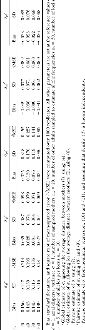
TABLE 1 Impact of the number ( no ) o f o ffspring sampled per mother o n the various global and pairwise estimators that use d ensity as an independently known value
ˆg1
a
ˆg2
b
ˆp1
c
ˆp2
d
ˆp3
e no Bias SD √ MSE B ias SD √ MSE B ias SD √ MSE B ias SD √ MSE Bias SD √ MSE 20 0.156 0.147 0.214 0 .035 0.087 0.093 0.325 0.318 0.455 ⫺ 0.049 0.077 0 .092 ⫺ 0.023 0 .085 0.088 40 0.143 0.130 0.193 0 .028 0.074 0.079 0.150 0.170 0.227 ⫺ 0.038 0.071 0 .081 ⫺ 0.025 0 .076 0.080 80 0.145 0.115 0.185 0 .031 0.064 0.071 0.076 0.119 0.141 ⫺ 0.030 0.061 0 .068 ⫺ 0.022 0 .068 0.071 160 0.139 0.116 0.181 0 .027 0.064 0.069 0.034 0.086 0.092 ⫺ 0.031 0.062 0 .069 ⫺ 0.026 0 .068 0.072 Bias, standard deviation, and square root of mean-squared error ( √ MSE) were computed over 1000 replicates. All o ther parameters are set a t the reference values density d ⫽ 1, axial dispersal variance ⫽ 1, number of sampled mothers nm ⫽ 20, number o f o ther adults sampled to estimate allelic frequencies nS ⫽ 30, number o f loci studied nL ⫽ 5, number of alleles per locus nA ⫽ 10. aGlobal estimate of , ignoring the average distance between mothers ( z ), using (4). bGlobal estimate of , allowing for the average d istance between mothers ( z ), using (6). cPairwise estimate of ,u si n g( 7 ). dPairwise estimate of , u sing (8) and (9). ePairwise estimate of , from nonlinear regression, (10) and (11), and assuming that density ( d ) is k nown independently.
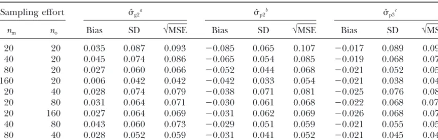
TABLE 2
Impact of sampling effort
Sampling effort ˆg2a ˆp2b ˆp3c
nm no Bias SD √MSE Bias SD √MSE Bias SD √MSE
20 20 0.035 0.087 0.093 ⫺0.085 0.065 0.107 ⫺0.017 0.089 0.090
40 20 0.045 0.074 0.086 ⫺0.065 0.054 0.085 ⫺0.019 0.068 0.071
80 20 0.027 0.060 0.066 ⫺0.052 0.044 0.068 ⫺0.021 0.052 0.056
160 20 0.006 0.042 0.042 ⫺0.042 0.033 0.054 ⫺0.021 0.038 0.044
20 40 0.028 0.074 0.079 ⫺0.038 0.071 0.081 ⫺0.025 0.076 0.080
20 80 0.031 0.064 0.071 ⫺0.030 0.061 0.068 ⫺0.022 0.068 0.071
20 160 0.027 0.064 0.069 ⫺0.031 0.062 0.069 ⫺0.026 0.068 0.072
40 80 0.043 0.060 0.073 ⫺0.029 0.051 0.059 ⫺0.021 0.055 0.059
80 40 0.028 0.052 0.059 ⫺0.031 0.041 0.052 ⫺0.021 0.045 0.049
Mean and standard deviation of the best global and pairwise estimators that use density as an independently known value for various sampling efforts,i.e., combinations of number of mothers (nm) and number of offspring
(no). All other parameters are set at the reference values densityd⫽1, axial dispersal variance ⫽1, number
of other adults sampled to estimate allelic frequenciesnS⫽ 30, number of loci studiednL⫽5, number of
alleles per locusnA⫽10.
aGlobal estimate of, allowing for the average distance between mothers (z), using (6). bPairwise estimate of, using (8) and (9).
cPairwise estimate of, from nonlinear regression, (10) and (11), and assuming that density (d) is known
independently.
deciding whether to use ˆd1 or ˆp3involves a tradeoff is indeed the case, especially for lower values of E, for which pairwise estimates yield an appreciable reduc-between one’s trust in the field estimate of density (dˆf)
and that quantity of genetic information available. tion in MSE; for very high values ofE, the reduction is minimal. The failure to achieve greater gains may be traceable to a feature that is common to all pairwise
DISCUSSION
analyses. The availability of multiple measures provides the impression that they should increase resolution, but We describe an effective means for estimating the
pollen distribution function, assuming a bivariate nor- each of those measures is extracted from a much smal-ler sample. Moreover, the collection of all pairwise mal distribution. Provided that density is known
inde-pendently, this study shows that it is possible to design φij-values is far from being an independent set of esti-mates (φjkis not independent ofφijandφik). In practice, estimators that are minimally biased and that have
enough precision to provide a trustworthy estimator of the collection of pairwise information provides a modest improvement on a single global average, which—while the average distance of pollen dispersal. Concerning
global estimates, we have shown that it is important to it ignores the detail—has the virtue of being based on a substantially larger sample size; the pairwise strategy take into account the average pairwise distance between
mothers, as a way of removing the potential bias that is better, but only mildly so. Since an iterative pairwise estimate is neither time- nor labor-intensive to obtain, occurs when the mothers are sampled at distances that
are too close. Among the pairwise estimates, the one particularly in view of the field and laboratory scope of such studies, it would always seem preferable to com-that exhibits the lowest MSE is the nonlinear regression.
The behavior of both global and pairwise estimates is pute one.
In practice, estimating adult reproductive density is a satisfactory even with 20 mothers and 20 offspring per
mother, but the best way to decrease mean-squared er- serious problem. For example, not all adults reproduce during a given year, and phenology is variable even ror is to increase the number of sampled mothers, rather
than the number of offspring per mother. Increasing within a year, so that not all parents can mate at the same time. There is also variation in male fecundity exclusion probability (E), by increasing either the
num-ber of loci or choosing more polymorphic loci, also within a population, as a function of age and size differ-ences, genetic differdiffer-ences, and microenvironmental fac-decreases MSE, but there is nothing much to be gained
by increasing this exclusion probability above 0.99, and tors. All of these factors contribute to a reduction in the effective density of reproducing individuals. In some for many purposes, a genetic battery that yields E ⬎
0.90 is quite adequate to the task. cases, it can be nearly impossible to count all adult plants belonging to a given species, in particular in This study was motivated by the idea that pairwise
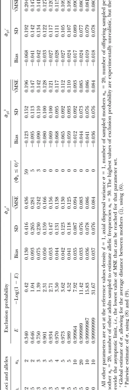
TABLE 3 Impact of the number o f loci ( nL ) a nd number o f alleles ( nA ) o n the best global a nd pairwise estimators that use d ensity as an independently known value Loci a nd alleles Exclusion p robability
ˆg2
a
ˆp2
b
ˆp3
c nL nA E ⫺ Log(1 ⫺ E ) B ias SD √ MSE ( ⌽ft ⱕ 0) d Bias SD √ MSE B ias SD √ MSE 2 2 0.340 0.42 0.130 0.416 0 .436 5 9 ⫺ 0.123 0.152 0.196 ⫺ 0.068 0.192 0.204 5 2 0.646 1.04 0.093 0.265 0 .281 5 ⫺ 0.095 0.113 0.147 ⫺ 0.041 0.142 0.147 3 3 0.750 1.39 0.075 0.230 0 .242 3 ⫺ 0.090 0.110 0.142 ⫺ 0.042 0.134 0.141 5 3 0.901 2.31 0.050 0.159 0 .166 0 ⫺ 0.080 0.100 0.128 ⫺ 0.033 0.122 0.127 3 5 0.934 2.71 0.053 0.147 0 .156 0 ⫺ 0.069 0.100 0.121 ⫺ 0.027 0.117 0.120 5 4 0.970 3.50 0.044 0.131 0 .138 0 ⫺ 0.068 0.095 0.117 ⫺ 0.028 0.111 0.115 4 5 0.973 3.62 0.042 0.123 0 .130 0 ⫺ 0.065 0.092 0.112 ⫺ 0.027 0.105 0.109 5 5 0.989 4.52 0.041 0.118 0 .125 0 ⫺ 0.059 0.093 0.110 ⫺ 0.024 0.107 0.109 5 1 0 0 .99964 7.92 0.035 0.087 0 .094 0 ⫺ 0.012 0.092 0.093 ⫺ 0.017 0.089 0.090 5 2 0 0 .999989 11.42 0.033 0.076 0 .083 0 ⫺ 0.044 0.073 0.085 ⫺ 0.024 0.077 0.080 10 10 0.99999987 15.83 0.036 0.078 0 .086 0 ⫺ 0.041 0.076 0.086 ⫺ 0.019 0.079 0.081 20 10 0.99999999 31.67 0.037 0.076 0 .084 0 ⫺ 0.036 0.076 0.084 ⫺ 0.018 0.078 0.080 All o ther parameters are set at the reference values density d ⫽ 1, axial dispersal variance ⫽ 1, number o f sampled mothers nm ⫽ 20, number of offspring sampled per mother np ⫽ 20, number o f o ther adults sampled to estimate allelic frequencies nS ⫽ 30. The highest values of exclusion probability are experimentally unrealistic, but they provide the asymptotic limit, i.e. , the lowest value o f M SE that can be reached for that parameter set. aGlobal estimate of , allowing for the average d istance between mothers ( z ), using (6). bPairwise estimate of , u sing (8) and (9). cPairwise estimate of , from nonlinear regression, (10) and (11), and assuming that density ( d ) is k nown independently. dNumber o f simulations (out of 1000) for which the estimated global ⌽ft was n egative and thus for which
ˆg2
could
n
ot
be
TABLE 4
Joint pairwise estimates ofdandfor various sampling efforts
Sampling effort dˆ1 ˆd1
nm no Bias SD √MSE Bias SD √MSE
20 20 0.151 0.726 0.742 0.016 0.266 0.267
40 20 ⫺0.097 0.325 0.340 0.061 0.165 0.176
80 20 ⫺0.116 0.201 0.232 0.051 0.105 0.117
160 20 ⫺0.120 0.133 0.179 0.048 0.076 0.089
20 40 ⫺0.052 0.419 0.422 0.043 0.183 0.188
20 80 ⫺0.068 0.385 0.390 0.045 0.161 0.167
20 160 ⫺0.079 0.348 0.357 0.038 0.134 0.140
All other parameters are set at the reference values densityd⫽1, axial dispersal variance ⫽1, number of other adults sampled to estimate allelic frequenciesnS⫽ 30, number of loci studiednL⫽5, number of
alleles per locusnA⫽10.dˆ1andˆd1are obtained from nonlinear regression using (10) and (11).
density can be nonhomogeneous across the landscape, can establish at least a numerical relation between⌽ft and dispersal distance for any dispersal function ( Aust-making any estimation of the effective density
approxi-mate and subject to uncertainty. Simply using the num- erlitzandSmouse2001a) suggests that this estimation procedure can be extended to a wider array of dispersal ber of individuals above a given size class can yield a
serious overestimate ofd and a serious underestimate functions. Since we can also account for genetic struc-ture among adults in the population (Austerlitzand of. The estimatordˆ1can be contrasted with the more
usual stem count; any discrepancy becomes an indicator Smouse2001b), we will also be able to design estimates that take that information into account. All such exten-of the extent to which various forms exten-of heterogeneity
have impacted on “effective male reproductive density,” sions will also require extensive testing. These are mat-ters that we will leave for future work.
de, which is likely to be less than the actual stem count.
We must keep in mind, however, that very large data This approach is essential since a good estimation of contemporary gene flow is essential to understand the sets are going to be required for reliable joint
estima-tion: large numbers of adults and offspring per adult, evolutionary processes that occur at the scale of a land-scape (Sork et al. 1999). It is the only way to infer along with a high-resolution (exclusion probability)
ge-netic battery. The increasing availability of numerous the consequence of various processes, which are often recent and man induced: fragmentation, loss of pollina-highly polymorphic loci at reasonable cost, however,
provides some hope that we can apply the method effec- tors, and extinction of local populations. Thus, only reliable inference of this instantaneous gene flow will tively in real situations.
This study shows that, at least for bivariate normal yield the possibility of predicting future changes for many species. TwoGener estimation should be useful pollen dispersion, the relationship between pollen
dis-persal distance and⌽ftcan be used to extract a useful in that context, because it allows us to gauge pollen flow, without typing all potential fathers in the popula-estimate of the decay parameter, . The fact that we
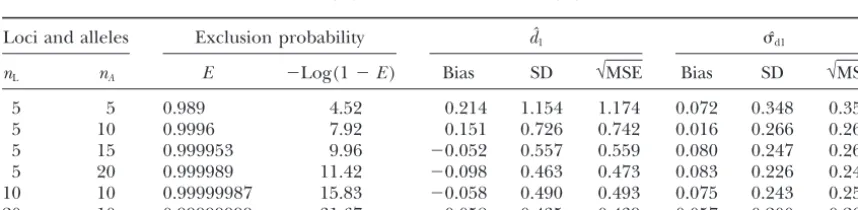
TABLE 5
Joint pairwise estimates (dˆ1,ˆd1) ofdandfrom nonlinear regression, (10) and (11), for various numbers of
loci (nL), and number of alleles (nA)
Loci and alleles Exclusion probability dˆ1 ˆd1
nL nA E ⫺Log(1⫺E) Bias SD √MSE Bias SD √MSE
5 5 0.989 4.52 0.214 1.154 1.174 0.072 0.348 0.355
5 10 0.9996 7.92 0.151 0.726 0.742 0.016 0.266 0.267
5 15 0.999953 9.96 ⫺0.052 0.557 0.559 0.080 0.247 0.260
5 20 0.999989 11.42 ⫺0.098 0.463 0.473 0.083 0.226 0.241
10 10 0.99999987 15.83 ⫺0.058 0.490 0.493 0.075 0.243 0.255
20 10 0.99999999 31.67 ⫺0.058 0.435 0.439 0.057 0.200 0.208
All other parameters are set at the reference values densityd⫽1, axial dispersal variance ⫽1, number
of sampled mothersnm ⫽ 20, number of offspring sampled per mothernp ⫽ 20, number of other adults
Kimura, M.,andG. H. Weiss,1964 The stepping stone model of
tion and even without having an estimate of adult
den-population structure and the decrease of gametic correlation
sity. Thus, it makes the method less labor intensive than
with distance. Genetics49:561–576.
alternative methods such as paternity analysis, and it Levenberg, A.,1944 A method for the solution of certain non-linear problems in least squares. Q. Appl. Math.2:164–168.
can be carried out over a broader stretch of landscape
Male´cot, G.,1948 Les mathe´matiques de l’he´re´dite´.Masson, Paris.
and during several years.
Marquardt, D. W.,1963 An algorithm for least-squares estimation of nonlinear parameters. J. Soc. Indust. Appl. Math.11:431–441. The authors thank A. J. Irwin, A. Kremer, V. L. Sork, and S.
Oddou-Press, W. H., S. A. Teukolsky, W. T. VetterlingandB. P. Flannery,
Muratorio for helpful commentary on the manuscript. P.E.S. was
1988 Numerical Recipes in C. The Art of Scientific Computing, Ed. supported by the New Jersey Agricultural Experiment Station (USDA/
2. Cambridge University Press, Cambridge, UK. NJAES-17106), McIntire-Stennis grant USDA/NJAES-17309, as well as
Rousset, F.,1997 Genetic differentiation and estimation of gene by National Science Foundation grant BSR-0089238. Most simulations flow fromF-statistics under isolation by distance. Genetics145: were performed on the UNIX machines of the Institut National de 1219–1228.
la Recherche Agronomique (Bordeaux and Jouy-en-Josas, France). Rousset, F.,2000 Genetic differentiation between individuals. J. Evol. Biol.13:58–62.
Slatkin, M.,1991 Inbreeding coefficients and coalescence times. Genet. Res.58:457–462.
LITERATURE CITED
Slatkin, M.,1993 Isolation by distance in equilibrium and non-equilibrium populations. Evolution47:264–279.
Austerlitz, F.,andP. E. Smouse,2001a Two-generation analysis
Smouse, P. E., R. J. Dyer, R. D. WestfallandV. L. Sork,2001 Two-of pollen flow across a landscape. II. Relation between⌽ft, pollen
generation analysis of pollen flow across a landscape. I. Male dispersal and inter-females distance. Genetics157:851–857.
gamete heterogeneity among females. Evolution55:260–271.
Austerlitz, F.,andP. E. Smouse,2001b Two-generation analysis
Sork, V. L., J. Nason, D. R. CampbellandJ. F. Fernandez,1999 of pollen flow across a landscape. III. Impact of adult population
structure. Genet. Res.78:271–280. Landscape approaches to the study of gene flow in plants. Trends
Chakravarti, A.,andC. C. Li,1983 The effect of linkage on pater- Ecol. Evol.142:219–224.
nity calculation, pp. 411–422 inInclusion Probabilities in Parentage Wolfram, S., 1999 The Mathematica Book. Wolfram
Media/Cam-Testing, edited byR. H. Walker.American Association of Blood bridge University Press, Champaign, IL/Cambridge, UK.
Banks, Arlington, VA. Wright, S.,1943 Isolation by distance. Genetics28:114–138.
Jamieson, A.,1994 The effectiveness of using co-dominant polymor- Wright, S.,1946 Isolation by distance under diverse systems of phic allelic series for (1) checking pedigrees and (2) distinguish- mating. Genetics31:39–59.
ing full-sib pair members. Anim. Genet.25(Suppl. 1): 37–44. Wright, S.,1951 The genetical structure of populations. Ann.
Eu-Jamieson, A.,andS. C. Taylor,1997 Comparisons of three proba- gen.15:323–354. bility formulae for parentage exclusion. Anim. Genet.28:397–