DOI: 10.1534/genetics.107.080002
Mapping Quantitative Trait Loci Affecting Susceptibility to Marek’s Disease
Virus in a Backcross Population of Layer Chickens
E. M. Heifetz,*
,1J. E. Fulton,
†N. P. O’Sullivan,
†J. A. Arthur,
†J. Wang,*
J. C. M. Dekkers* and M. Soller
‡*Department of Animal Science and Center for Integrated Animal Genomics, Iowa State University, Ames, Iowa 50011,
†Hy-Line International, Dallas Center, Iowa 50063 and‡Department of Genetics,
The Hebrew University, Jerusalem 91904, Israel Manuscript received August 7, 2007 Accepted for publication October 15, 2007
ABSTRACT
Marek’s disease (MD), caused by the oncogenic MD avian herpes virus (MDV), is a major source of economic losses to the poultry industry. A reciprocal backcross (BC) population (total 2052 individuals) was generated by crossing two partially inbred commercial Leghorn layer lines known to differ in MDV resistance, measured as survival time after challenge with a (vv1) MDV. QTL affecting resistance were identified by selective DNA pooling using a panel of 198 microsatellite markers covering two-thirds of the chicken genome. Data for each BC were analyzed separately, and as a combined data set. Markers showing significant association with resistance generally appeared in blocks of two or three, separated by blocks of nonsignificant markers. Defined this way, 15 chromosomal regions (QTLR) affecting MDV resistance, distributed among 10 chromosomes (GGA 1, 2, 3, 4, 5, 7, 8, 9, 15, and Z), were identified. The identified QTLR include one gene and three QTL associated with resistance in previous studies of other lines, and three additional QTL associated with resistance in previous studies of the present lines. These QTL could be used in marker-assisted selection (MAS) programs for MDV resistance and as a platform for high-resolution mapping and positional cloning of the resistance genes.
M
AREK’S disease (MD) of chickens is caused by theoncogenic MD avian herpes virus (MDV). When originally described in 1907 MD manifested as a mild endemic paralytic disease. MD today, however, is an acute highly contagious disease causing tumors in multiple
visceral organs (Nair 2005) and is a major source of
economic losses to the poultry industry (Morrowand
Fehler2004). The disease is well controlled by
vacci-nation with the highly effective ‘‘Rispens’’ vaccine, but ever more virulent strains are constantly evolving and have already ‘‘broken’’ three vaccines (Nair2005). There
is thus great importance to developing methods of control based on well-documented genetic resistance to
MDV (reviewed in Bumsteadand Kaufman2004).
Current genetic methods for improving resistance to MDV are based on family selection, which is expensive in terms of time, facilities, and selection space and poses the ethical dilemma of challenging large numbers of birds with a virulent pathogen. Identification of quan-titative trait loci (QTL) for MDV resistance will allow marker-assisted selection (MAS) on an individual bird level, without need for routine challenge. This will greatly enhance efficacy of selection, reduce costs by orders of
magnitude, and provide a platform for eventual identi-fication of the quantitative trait genes (QTG) corre-sponding to the mapped QTL. QTL mapping can also provide information on epistatic interactions among the identified QTL, further increasing the potential for ge-netic improvement.
Polymorphic alleles at the MHC (B blood group) on
chromosome 16 (reviewed in Weigendet al.2001), the
growth hormone gene (GH1) located on chromosome 1 (Kuhnleinet al. 1997; Liuet al. 2001), and the stem
lymphocyte antigen 6 complex locus E (LY6E) located
on chromosome 2 (Liu and Cheng2003) have been
shown to affect resistance to MDV. A series of QTL map-ping studies for MDV resistance have been carried out under experimental challenge in crosses of two highly inbred White Leghorn lines, 6 and 7 (Avian Disease and Oncology Laboratory, ADOL), known to differ widely in susceptibility to MDV (Vallejoet al. 1998). Mapping in
a backcross population of these lines identified a QTL
for MDV resistance on chromosome 1 (Bumstead
1998); mapping in an F2cross of these lines identified QTL for MDV resistance on chromosomes 1, 2, 4, 7, and 8 (Vallejoet al. 1998; Yonashet al. 1999).
In this study, QTL affecting resistance to MDV were mapped by selective DNA pooling in a large reciprocal backcross (BC) population generated by crossing two partially inbred commercial Leghorn layer pure lines 1Corresponding author:Department of Molecular Biology, Ariel
Univer-sity Center of Samaria, Ariel 44837, Israel. E-mail: [email protected]
known to differ in resistance to this virus. One goal of this research was to determine if the QTL uncovered in the Leghorn lines investigated by Vallejoet al.(1998)
and Yonashet al.(1999) were also a source of genetic
variation in these commercial Leghorn lines.
MATERIALS AND METHODS
Resource population: Stocks: The experiment was carried
out using facilities and two commercial Leghorn lines (hence-forth, line 1 and line 2) of Hy-Line International (hence(hence-forth, Hy-Line). Both lines were partially inbred and fixed for alter-native blood-type (BT) groups; B2/B2 in line 1 and B15/B15 in line 2. A previous screen of 102 microsatellite markers on these lines showed that 60 and 80% of the markers were fixed in line 1 and line 2, respectively. Both line 1 and line 2 have been subjected to selection for resistance to MD, and both are relatively resistant when compared to field strains. However, in experiments performed in 2000, 2003, and 2005 under the same challenge protocol as this study, absolute mortality of line 1 at the end of the test (19 w) was higher than that of line 2, by 41.4, 42.7, and 21.7%, respectively. Thus, under this challenge line 2 is distinctly more resistant than line 1. The 2003 test also included the F6generation of a cross of the two lines. This population exhibited a high level of mortality, with absolute mortality being 36.8% greater than that of line 2 and only 5.9% less than that of line 1 ( J. A. Arthur, N. P.
O’Sullivan, K. K. Kreagerand Hy-Line, unpublished data).
Experimental populations: To provide replication and some indication of QTL segregation within the two lines, each BC population was produced in five independent replicates, termed ‘‘families,’’ as follows. Five line-1 males were each pair mated with a single different line-2 female to produce an F1 generation consisting of five independent full-sib F1families. A group of seven full-sib F1males from each of the five families were each pen mated to a group of 18–20 females from line 1 (total 35 males and 100 females) to produce a backcross population consisting of five independent families with line 1 as the recurrent parent (henceforth, BC-1), each family consisting of the progeny of seven full-sib F1males and 18–20 line-1 females. Six months later, the same five groups of F1 males were each again pen mated to a group of 18–20 females from line 2 to produce the reciprocal backcross population (henceforth, BC-2), also consisting of five independent families. The BC-1 included 837 birds with 163–176 chicks per family; BC-2 included 1215 birds with 234–258 chicks per family. Two BT genotypes, B2/B2 and B2/B15 were present in BC-1, and two BT genotypes, B2/B15 and B15/B15 were present in BC-2.
MD challenge test:Day-old BC-1 chicks were vaccinated with bivalent HVT/SB-1 vaccine (Merial Select, Gainesville, GA) and housed in brooder cages. This is the vaccine that was used prior to the current Rispens vaccine, and hence provides only partial protection to the chicks. At 7 days the chicks were inoculated subcutaneously with 500 PFU of the very virulent (vv1) strain (648A) of the MDV (Witter 1997) and then
transferred to a floor facility challenge house. At 3 weeks of age, blood samples for blood typing and DNA isolation were collected and stored. Age at mortality was recorded on all chicks as an indicator of resistance to MDV until 116 days of age, at which time the test was terminated. This same pro-cedure was repeated for BC-2 six months later, except that the test was terminated at 138 days of age. This test has been shown to result in data with substantial heritability (0.10–0.22) for sire progeny averages on the basis of 30 daughters ( J. E. Fulton, P. Settarand Hy-Line, unpublished data).
DNA extraction and pool construction:At 3 weeks of age, blood was collected from the jugular vein with 22-gauge needles in syringes containing EDTA. DNA was isolated from the blood using proteinase K digestion, salt, and ethanol precipitation (maniatiset al.1982). The OD
260/280ratios were subsequently determined. Each sample was diluted to 50 ng/ml DNA concentration, retested for DNA content, and further diluted to 25 ng/ml. Pools of DNA were made by combining equal volumes of the 25 ng/ml samples from each of the birds iden-tified as belonging to the pool (see below).
To reduce the number of genotypings, selective DNA pooling (Darvasi and Soller1994; Lipkinet al. 1998) was
used. This method has proven very accurate in the Hy-Line laboratory (Lipkinet al. 2001). Because of the known effect of
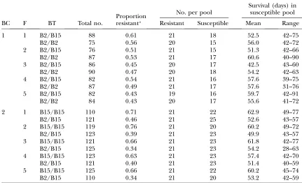
the MHC BT on MDV resistance, pools of DNA of resistant and susceptible birds were constructed within each BC 3BT3 family combination (CBF), as shown in Table 1. Progeny within each CBF combination were ranked by age at mortality, or designated as ‘‘survivors’’ if they survived until termination of the challenge test with no obvious symptoms of MD. The susceptible pools within eachCBFcombination consisted of the 20% of birds with earliest age to mortality. For all CBF combinations, the number of survivors was.20%. Hence, to match the number of birds in the susceptible pools, 21 (on average 20%) of the surviving birds were chosen at random for each family. This gave a total of 2 BC32 BT/BC35 families/ BC–BT combination32 tails (resistant and susceptible)/CBF combination¼40 pools.
Genotypic data: Pools were genotyped for a total of 198 microsatellite markers chosen so that overlap in alleles be-tween the two parent lines was absent or limited to a single allele. Since not all markers were informative for both back-crosses, 180 markers were used in BC-1, and 176 in BC-2; 158 markers were common to both BCs.
Marker locations were assigned according to the consensus 2000 chicken linkage map (http://iowa.thearkdb.org/). When there was a discrepancy between the consensus map and the chicken sequence (http://www.ensembl.org/Gallus_gallus/ index.html), the order of the markers was based on the se-quence. In these cases, as well as cases of markers that were not on the consensus map, additional markers flanking the questioned marker were identified that were in the same order in the sequence and the consensus map. The questioned marker was then positioned on the consensus map propor-tionally to these two markers. Linkage data derived from Hy-Line populations (Wang 2003) were available for
chro-mosomes 4, 15, and Z, and these were used for analysis, since they gave a better fit to the sequence than did the linkage data of the consensus map. In addition, the study included five markers that were assigned to specific chromosomes but did not have specific locations and four markers that were not assigned to chromosomes.
Genome coverage: The regions bracketed by the most proxi-mal and the most distal markers on each of the 15 chromo-somes tested with three markers or more, gave a total of 2180 cM. To this can be added on average 20 cM for each of these 15 chromosomes (total 300 cM) to account for chromosome coverage from the most proximal and the most distal markers to the chromosome ends, and another 20 cM for each of the remaining 10 chromosomes that were covered by only one or two markers (total 200 cM) to give total genome coverage of
2680 cM. Thus, approximately two-thirds of the 4000 cM chicken genome (Groenenet al2000) was scanned in this
study.
Genotyping methods:For all markers, allele frequencies in the pools were estimated by densitometric PCR. Following Lipkin
micro-satellite markers and also for differential amplification be-tween alleles when present.
Statistical methods: The basis for all statistical tests of
significance of marker–QTL linkage were the differences (Dhijk-values) in densitometric estimates of marker allele fre-quencies between the resistant and susceptible pools for the hth marker, ith backcross, jth blood-type, and kth family (MCBF)hijkcombination. All tests were carried out separately for the two backcrosses and for the combined data across the two backcrosses. Unless specified otherwise, the term ‘‘crosses’’ will refer to results of all three calculations (i.e., for BC-1, BC-2, and the combined data). The Dhijk were evaluated for sig-nificance using a variety of statistical tests (Z-test, chi square, interval analysis, ANOVA, and nonparametric sign test), each of which explored a somewhat different aspect of the data. In particular, theZ-test that was implemented (see details in the following) evaluates the main effect of a marker allele on D-values acrossCBFcombinations. Thus, theZ-test is sensitive to main effects and provides an estimate of the direction of effect of specific alleles, but is insensitive to marker–blood-type–family interaction effects. The chi-square test analyzes D-values within eachCBFcombination, allowing for different directions of effects and is, therefore, less sensitive to main effects than theZ-test but more sensitive to interaction effects. TheZ- and chi-square tests are both based on analysis of single markers. To take into account the additional information present in adjacent markers,Dhijk-values for all markers on a chromosome were analyzed jointly using a likelihood-based method equivalent to interval analysis (IA) that was described in Wanget al(2007). By analyzing eachCBFcombination as a
separate family, the IA shares with chi square its sensitivity to interaction effects but is less powerful than theZ-test to detect
main effects. The three tests just described (Z, x2, and IA) make use ofD-values divided by their standard error (SE). Two additional tests: a three-way ANOVA and a nonparametric sign test were also used. These, although based on the same D-values as above, each use a different basis to test significance (see details in the following), in this way providing an additional control to the statistical calculations. Both ANOVA and the sign test share with the Z-test its sensitivity to main effects and insensitivity to interaction effects.
The individual statistical tests are now presented in turn. Chi square: A chi-square test was calculated across all 10 blood-type3family (BFjk) combinations within each marker3 cross (MChi) combination, as
x2 hi¼
X
j
X
k
Z2
ðhiÞjk;
where the parentheses in the subscript ofZ(hi)jkindicate that the summation was carried out separately across all BFjk combinations within eachMChicombination
Zhijk¼Dhijk=SEðDhijkÞ;
Dhijk¼dFhijk1dFhijk2:
dFhijk1 anddFhijk2are the densitometric estimates of the fre-quency of the marker allele derived from line 2 in the resistant and susceptible pools, respectively. SE(Dhijk) are the standard errors of theDhijk½seeappendix afor derivation of SE(Dhijk).
Summation, as noted, was across all 10 (BF)jkcombinations within eachMChicombination. Consequently, the degrees of freedom (d.f.) was generally 10, but was occasionally less (4–9) according to the number of BFjk combinations for which TABLE 1
Pool composition according to backcross (BC), family (F), and blood type (BT)
Proportion resistanta
No. per pool
Survival (days) in susceptible pool
BC F BT Total no. Resistant Susceptible Mean Range
1 1 B2/B15 88 0.61 21 18 52.5 42–75
B2/B2 75 0.56 20 15 56.0 42–72
2 B2/B15 76 0.51 21 15 51.3 42–66
B2/B2 87 0.53 21 17 60.6 40–90
3 B2/B15 86 0.45 20 17 42.5 43–60
B2/B2 90 0.47 20 18 54.2 42–63
4 B2/B15 82 0.54 21 16 57.6 39–75
B2/B2 87 0.49 21 17 57.6 31–76
5 B2/B15 82 0.43 19 16 59.7 42–91
B2/B2 84 0.43 20 17 55.6 41–72
2 1 B15/B15 110 0.71 21 22 62.9 49–77
B2/B15 121 0.46 21 25 52.6 43–57
2 B15/B15 119 0.76 21 20 60.2 49–72
B2/B15 123 0.39 21 23 49.9 43–57
3 B15/B15 121 0.66 21 23 61.8 42–77
B2/B15 125 0.34 21 23 54.2 28–63
4 B15/B15 123 0.63 21 23 57.4 42–70
B2/B15 121 0.40 21 23 51.4 40–59
5 B15/B15 125 0.66 21 22 60.2 45–74
B2/B15 110 0.34 21 20 53.2 42–59
densitometric estimates of allele frequency were obtained within an individualMChicombination.
The P-value for the chi-square test was taken from the distribution of chi square by degrees of freedom. For chi-square analysis of the combined backcrosses,x2
hi and degrees of freedom were simply summed across BC-1 and BC-2.
Z-test:AZ-test for a difference in allele frequencies between resistant and susceptible was calculated across all 10 blood-type3family (BFjk) combinations within each marker3cross (MChi) combination, as
Zhi ¼wDhi=SEðwDhiÞ;
wherewDhiis the weighted averageD-value across the resistant and susceptible pools of the 10BFjkcombinations within each of the MChi combinations, weighted by the number of individuals in each pool, and SE(wDhi) is its standard error
½seeappendix afor derivation ofwD
hiand SE(wDhi). TheP-value for theZ-test was obtained from the standard normal distribution. For theZ-test of the combined BC data, an average (wDh) of thewDhi-values across the two BCs and its standard error were used (seeappendix afor details).
Interval analysis: The interval analysis was implemented using the likelihood-based method of Wanget al.(2007). In
this analysis, the differentBFjkcombinations within crosses were treated as independent observations, and the joint like-lihood for each cross was maximized with regard to the para-meters of QTL location and estimate of the QTL frequency P(Q(hi)jk) in the upper tail at the maximum position, where the parentheses indicate that the calculation was for eachMChi combination separately, and the underline indicates that the maximization was across all BFjk combinations within each
MChi combination. This estimate was used to calculate an estimate ofD(hi)jk), namelyD(hi)jk¼P(Q(hi)jk)(1P(Q(hi)jk)). TheseD-values were then used to estimate the QTL effect for each backcross as described later. The analysis was carried out separately for each backcross and for the combined data.
ANOVA:A three-way ANOVA was implemented using the Fit Model option in the JMP 5.1.2 statistical package (1989–2004, SAS Institute). Only main effects were tested because of limited degrees of freedom, using the following models:
Model 1:Dh(i)jk¼ m 1 Mh1 BTj1 Fk 1 eh(i)jk, where the parentheses in the subscript indicate that the model was run separately for the individual backcross analyses.
Model 2:Dhijk¼ m1Mh1 BCi 1BTj1 Fk 1ehijk, for the combined analysis.
To the extent that some of the interactions are real, this will increase the error term, decreasing the significance of the results. However, not accounting for correlations that are expected to exist betweenD-values from linked markers will increase the significance since there are fewer effective degrees of freedom than assumed. Hence, these two effects will counteract to some extent. The ANOVA also provides esti-mates of the magnitude and direction of the main marker effect across BFjk combinations within MChi combinations (model 1), or main marker (Mh) effects acrossCBFijk combi-nations (model 2) and tests whether these are significantly different from zero.
Nonparametric sign test:In addition to the four statistical tests listed above, a nonparametric sign test (Walpoleand Myers
1978) was used in the initial stage of the analysis for compu-tational ‘‘quality control.’’ This test was based on the expecta-tion that when marker–QTL linkage is present, the sign of the D(hi)jk-values for that marker across all tenBFjkcombinations within theMChimarker–cross combination will be the same (all positive or all negative); while under the null hypothesis of no linkage, the sign of theD(hi)jk-values should be equally
distributed among positive and negative values. Major dis-crepancies between the markerP-values from the sign test and the markerP-values from the ANOVA orZ-tests were invaluable in alerting us to problems with procedures, data, or specific calculations. However, because the sign test tracks the same effects as ANOVA and theZ-test, but has less power than either, results with this test are not presented or discussed further.
Accounting for multiple tests: To take into account the
multiple-test situation while retaining power, a 20% ‘‘pro-portion of false positive’’ (PFP) threshold was used to de-termine the critical comparisonwise error rate (CWER) or P-value for declaring marker–QTL linkage (Fernandoet al.
2004). For the IA test, the PFP calculation was done using all IA tests that were conducted on a chromosome at 1-cM intervals, as in the range of CWER values.0.001, there was a fairly smooth and monotonic relationship between rank number and PFP (see also Figure 2 of Leeet al. 2002).
Application of the PFP method requires prior estimation of the number of tests for which the null hypothesis is true (tN), since only such tests can provide a false positive. This was done following the algorithm presented in Nettletonet al. (2006).
Given an estimate oftN, PFP for theith test is calculated as: PFPi¼(PitN)/Ri, wherePiis theP-value of theith test, when the tests are ranked by theirP-values from lowest to highest, andRiis the rank number of theith test. The number of tests representing false null hypotheses,fN,i.e., representing true marker–QTL linkages, can then be estimated asfN¼NtN and effective power asoN/fN, whereoNis the number of tests that are significant according to the designated significance level.
Estimating the effects of markers and QTL on survival
time: For each marker, M, with alleles M1 and M2 derived
from line 1 and line 2, respectively, each pool contains two genotypic groups: eitherM1M1andM1M2for BC-1 orM2M2 andM1M2for BC-2. With standard selective genotyping, the observed allele substitution effect is the observed quantitative difference between the two genotypic groups,aP, taken over the selected tails of the population. With selective DNA pool-ing,aPis estimated from theD-values (Darvasiand Soller
1994). Darvasiand Soller(1992, 1994) pointed out that in
both cases,aPis an exaggerated estimate of the actual sub-stitution effect in the population as a whole,aT, and provided an expression to estimateaTfromaPwith selective genotyping for a normally distributed trait. With appropriate modifica-tions, this expression was adapted for the present data set (see
appendix bfor derivation). When applied to simulated
sur-vival data, the Darvasiand Soller(1994) expression appears
to provide estimates of allele substitution effects that show a slight positive bias (10% greater) relative to the simulated effects. The same procedure was also used for the IA to estimate effects at QTL using estimates of D-values at the estimated QTL location obtained from that analysis (see also Wanget al.
2007).
Defining QTL containing chromosomal regions (QTLR) and testing for differences in allele substitution effects at the
QTLR:Because many of the markers were rather closely spaced,
it is expected that a number of markers constituting a ‘‘block’’ may present significance if they span a chromosomal region containing a QTL. Indeed, examining the results showed that significant markers often appeared in blocks of two or more consecutive significant markers. Each such block was taken to constitute a QTL-containing region (QTLR). Blocks of signif-icant markers were generally separated or flanked by runs of two or more consecutive nonsignificant markers. Each such block of nonsignificant markers was taken to define a chromosomal region from which QTL were absent (non-QTLR).
they each present estimates for the allele substitution effect at the QTL. Consequently, differences in allele substitution effects of the various QTL could be tested by an ANOVA in which QTLR are taken as main effects and markers within QTLR as replicates. Since estimated marker effects for a given MChi combination are directly proportional to theD-values from which they are derived, differences in allele substitution effects at the different QTLR within the individual backcrosses were tested in practice by a one-way ANOVA of their respective marker D(hi)jk-values, with QTLR as the main effect and estimated markerD(hi)jk-values within a given QTLR taken as the individual variables, where the parentheses in the sub-script indicate that the analysis is done withinMChi combina-tions, and the underline in the subscript indicates that the analysis is done across allBFjkcombinations within a given
MChicombination. ANOVA for the combined backcross was implemented in a similar way, except that analysis was done across allCBFijkcombinations within a givenMh.
Significance of difference in map location of QTL identified in this study and in other independent studies
reported in the literature:A major objective of this study was
to examine whether the QTL identified in experimental populations, were relevant with respect to QTL segregating in commercial populations. This was implemented as follows. To determine whether QTL reported on the same chromo-some in two independent studies, S1 and S2, represent the same or different QTL, letL1be location of the QTL identified in S1, andL2be the location of the QTL identified in S2;N1and
N2, the total size of the respective mapping populations; andd, the standardized allele substitution effect at the QTL (under the null hypothesis that the QTL location anddare the same in the two populations). Then, significance of the difference in locationsL1andL2, with type I errora, is given by the integral of the standard normal curve fromZa/2to infinity, where
Za=2¼DL=SEðDLÞ
DL¼L1L2, is the difference in map location between the QTL identified in the two studies, SE2(D
L) ¼ SE2(L1) 1 SE2(L
2), and SE(L1) and SE(L2) are the SE of QTL map location for the QTL at locationL1andL2,respectively.
For F2 and BC populations and a saturated marker map, SE(L) can be estimated from the published expressions for the 95% confidence interval (C.I.) of QTL map location (Darvasi
and Soller1997; Wellerand Soller2003), namely: C.I.95(L,
F2)¼1500/Nd2; C.I.95(L, backcross)¼3000 cM/Nd2. Noting that the C.I.95was set equal to 4SE(L), we have
SEðL;F2Þ ¼375 cM=Nd2;
SEðL;BCÞ ¼750 cM=Nd2:
RESULTS
In BC-1 the two BT genotypes (B2/B2 and B2/B15) were virtually identical in proportion of survivors, and differed by only 4.1 days (not significant by ANOVA) in favor of B2/B2 for mean survival time of the birds in the susceptible pool. In BC-2, however, B2/B15 was
signif-icantly more susceptible than B15/B15 (P , 0.01 by
ANOVA): the proportion of survivors at the end of the test was 29.8% less than for B15/B15 (absolute value), and mean survival time of the birds in the susceptible pool was shorter by 8.2 days (Table 1).
On the basis of the ANOVA analysis, family effect approached significance in BC-1 and was borderline
significant in BC-2 and the combined analysis (P ,
0.05). The marker effect was highly significant in all populations.
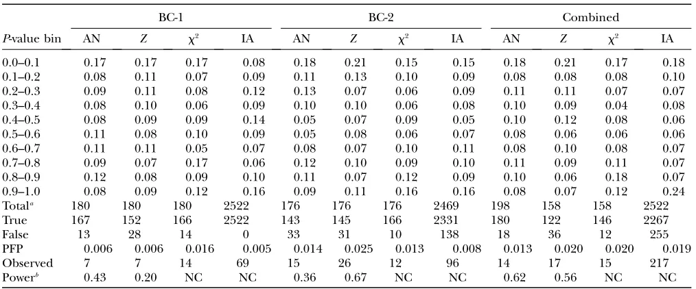
Table 2 shows the distribution of the P-values of the various statistical tests, in bins of width 0.10. On the null hypothesis, the proportion of tests in eachP-value bin is
expected to be 0.10. For ANOVA,Z, chi square and IA
there was a highly significant excess of tests in the lowest
P-value bin (0–0.1) in all data sets (BC-1, BC-2, and the combined data) except for IA in BC-1.
For the BC-1, BC-2, and combined data, IA also showed a highly significant excess of tests in the highest
P-value bin (0.9–1.0); a similar tendency, but not as
strong or as significant was presented by the chi-square test. This excess cannot be due to linkage. Thus, the IA and chi-square tests appear to be conservative, which could be caused by some of their underlying assump-tions not being met.
On the basis of the results in Table 2, the CWER
P-values corresponding to the 0.20 PFP threshold level
were calculated. These differed among crosses and test statistics but when averaged across all three data sets, threshold P-values for the various statistical tests were quite similar, being 0.011, 0.019, 0.016, and 0.011 for
ANOVA, Z, chi square, and IA, respectively. These
averaged thresholds were used to determine signifi-cance for the individual tests.
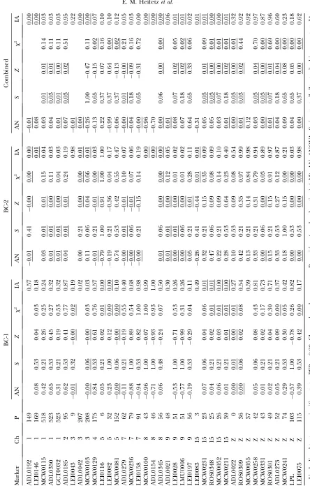
Table A1 shows markers that reached significance at PFP¼0.20 for at least two statistical tests (not including the sign test). These could be two different tests in any one of the three data sets, or the same test in any two of
the three data sets. For these markers, CWER P-values
are given for each of the four tests, according to cross and analysis. Comparing the observed number of sig-nificant results, with the estimated number of false null hypotheses (Table 2), provides estimates of the power of
the analyses. For ANOVA andZ, power estimates ranged
from 0.36 to 0.67, with a mean of 0.52 over all crosses. For chi square and IA, the conservative nature of the tests may be affecting power estimates in unknown ways, and hence the results are not presented.
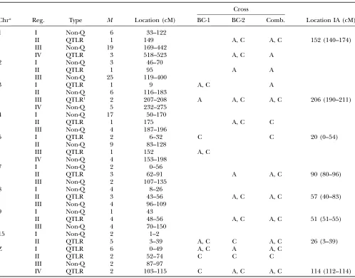
Table 3 shows the QTLR and non-QTLR defined in this way. An exception was made for chromosome Z, where QTLR I and II were not separated by nonsignif-icant markers. In this case, two QTL were assumed on the basis of the overall length of the significant region which extended from 0 to 74 cM.
A total of 20 significant QTLR 3 BC combinations
were uncovered, located on 10 of the 25 chromosomes included in the genome scan (GGA1, 2, 3, 4, 5, 7, 8, 9, 15, and Z). Fifteen chromosomes, with one to four markers per chromosome, did not carry any significant
markers (see Table 3, footnote a, for details). Of the
(47.7%) were significant only in BC-2. Thus, a total of 15 different QTLR were uncovered. Of the 20 significant
QTLR3BC combinations, 4 (20%) were significant for
the ANOVA and/orZ-tests only, 5 (25%) were
signifi-cant for x2 and/or IA tests only, and 11 (55%) were
significant for both ANOVA/Z-and x2/IA tests. Thus,
within the individual BCs, 75% of the uncovered QTL had a significant additive component, while only 25% were strongly interactive, with little or no additive ef-fects. A virtually identical picture was seen for the 14 QTLR found significant in the combined analyses.
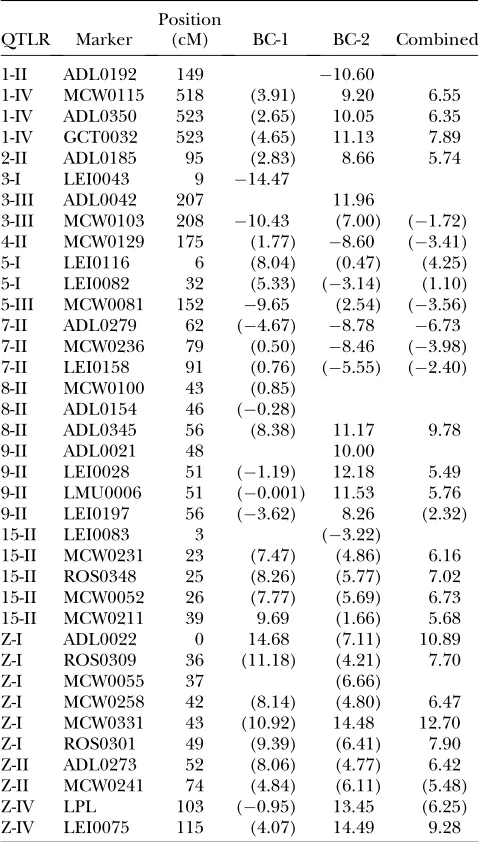
The effect on survival time was calculated separately
for eachM3BC3Fcombination in each of the QTLR
as described inappendix b, using the samewDhi-value as
used for theZ-test for thatM3BC3Fcombination, and
using the estimatedD-value at the marker for the IA.
The average survival time over allM3Fcombinations of a given QTLR within crosses are presented in Table A2, separately by cross. When all markers in the QTLR regions were considered, 73.3, 78.1, and 77.8% of alleles from line 2 were associated with positive (increasing) effects on survival time for the BC-1, BC-2, and the combined analysis, respectively. When all markers in the non-QTLR regions were considered (data not shown),
percentages of markers with positive D-values were
significantly lower (P , 0.0001 by chi-square
contin-gency test), at 55.8, 62.7, and 56.7%, respectively. This indicates that in the QTLR regions, positive effects of the line 2 alleles on survival time predominated, as expected.
Examination of estimated effects for individual markers within QTLR (Table A2) showed a relatively high consistency of effects across markers within QTLR within crosses and major differences between QTLR within crosses; in particular some QTLR were charac-terized by positive effects and others by negative effects. The ANOVA analyses showed that for all crosses and for the IA, differences among QTLR were highly significant
(P,0.0001) (data not shown). On this basis, the mean
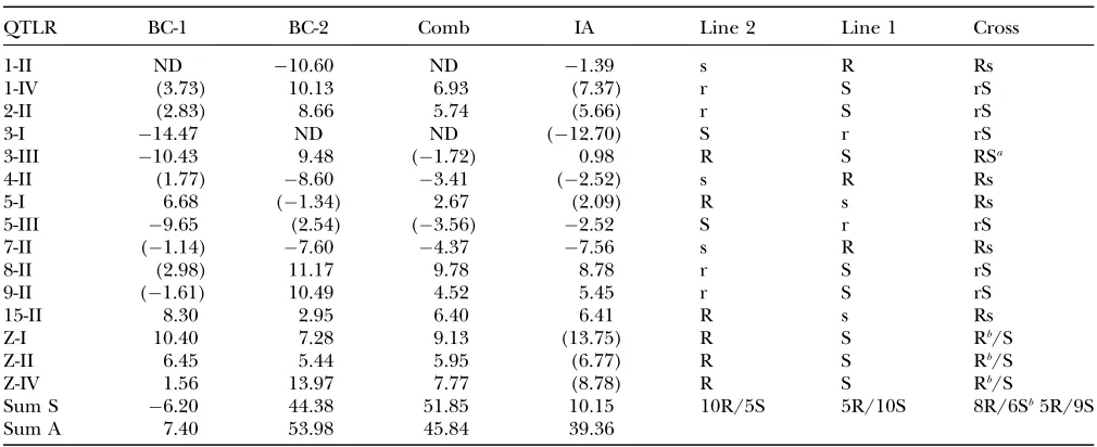
effect on survival time of all markers within a QTLR was taken to represent the effect of the QTLR on survival time. These are shown in Table 4, separately for BC-1, BC-2, combined analysis, and IA. Effects are given for all 15 defined QTLR, whether or not they were significant in the particular population or analysis, but effects based on nonsignificant QTLR are shown in parenthe-ses. Effects in BC-1 and BC-2 often differed greatly. Effects in combined and IA were generally very similar and approximately equal to the mean effect across BC-1 and BC-2.
Considering all QTLR, whether significant or not: 9 of 14 effects were positive for BC-1, 10 of 14 effects were
TABLE 2
Distribution of theP-values, estimated number of true and false null hypotheses of total tests, 0.20 PFP significance
thresholds, number of observed significant results, and estimated power for ANOVA (AN),Z-test (Z),
chi square (x2) and interval analysis (IA), according to cross
BC-1 BC-2 Combined
P-value bin AN Z x2 IA AN Z x2 IA AN Z x2 IA
0.0–0.1 0.17 0.17 0.17 0.08 0.18 0.21 0.15 0.15 0.18 0.21 0.17 0.18
0.1–0.2 0.08 0.11 0.07 0.09 0.11 0.13 0.10 0.09 0.08 0.08 0.08 0.10
0.2–0.3 0.09 0.11 0.08 0.12 0.13 0.07 0.06 0.09 0.11 0.11 0.07 0.07
0.3–0.4 0.08 0.10 0.06 0.09 0.10 0.10 0.06 0.08 0.10 0.09 0.04 0.08
0.4–0.5 0.08 0.09 0.09 0.14 0.05 0.07 0.09 0.05 0.10 0.12 0.08 0.06
0.5–0.6 0.11 0.08 0.10 0.09 0.05 0.08 0.06 0.07 0.08 0.06 0.06 0.06
0.6–0.7 0.11 0.11 0.05 0.07 0.08 0.07 0.10 0.11 0.08 0.10 0.08 0.07
0.7–0.8 0.09 0.07 0.17 0.06 0.12 0.10 0.09 0.10 0.11 0.09 0.11 0.07
0.8–0.9 0.12 0.08 0.09 0.10 0.11 0.07 0.12 0.09 0.10 0.06 0.18 0.07
0.9–1.0 0.08 0.09 0.12 0.16 0.09 0.11 0.16 0.16 0.08 0.07 0.12 0.24
Totala 180 180 180 2522 176 176 176 2469 198 158 158 2522
True 167 152 166 2522 143 145 166 2331 180 122 146 2267
False 13 28 14 0 33 31 10 138 18 36 12 255
PFP 0.006 0.006 0.016 0.005 0.014 0.025 0.013 0.008 0.013 0.020 0.020 0.019
Observed 7 7 14 69 15 26 12 96 14 17 15 217
Powerb 0.43 0.20 NC NC 0.36 0.67 NC NC 0.62 0.56 NC NC
a
The total number of tests in the combined analysis represents the total number of markers across either of the two BC pop-ulations for ANOVA, but the number of markers common to both BC poppop-ulations for theZand chi-square tests. For IA, the number of tests represents the maximum map size in centimorgans, as determined by the most proximal and most distal markers of each chromosome. These markers were identical for BC-1 and BC-2, with one exception, in which the BC-1 marker was 53 cM closer to the chromosome end than the BC-2 marker. Hence, the total number of tests in the combined IA (2522), was the same as that for the BC-1 population.
positive for BC-2, 9 of 13 effects were positive for the combined analysis, and 10 of 15 effects were positive for IA. Considering only significant QTLR, 5 of 8 significant QTLR were positive in BC-1, 9 of 12 were positive in BC-2, and 9 of 11 were positive in the combined analysis, but only 3 of 6 significant QTLR were positive in the IA. Thus, in the BC-2 and combined analysis there was a clear predominance of positive effects associated with line 2 alleles, as expected from the difference between the parental lines. In BC-1, however, a relatively large number of negative effects were associated with line 2 alleles.
SinceD-values were calculated as the frequency of the line 2 allele in the resistant pools minus frequency of the line 2 allele in the susceptible pools, positive QTLR
effects on survival time represent positive effects of the line 2 QTL alleles on resistance, and negative effects of QTLR on survival time represent negative effects of the line 2 QTL alleles on resistance. Thus, summing the effects of all QTLR within a population or analysis (whether significant or not) provides an estimate of the expected difference in mean survival time between line 2 and line 1, which can be attributed to the identified QTL. When this is done, estimates of 7.4, 54.0, 45.8, and 39.4 days are obtained for BC-1, BC-2, the combined analysis, and IA estimates, respectively. The estimates for BC-2, the combined analysis, and IA are roughly similar and indicate a difference in survival time for line
2 and line 1 of 46 days, under the conditions of
the experiment. It may be advisable to reduce this
TABLE 3
Chromosomal regions that contain QTL (QTLR) and that do not contain QTL, according to cross and statistical test
Chra Reg. Type M Location (cM)
Cross
BC-1 BC-2 Comb. Location IA (cM)
1 I Non-Q 6 33–122
II QTLR 1 149 A, C A, C 152 (140–174)
III Non-Q 19 169–442
IV QTLR 3 518–523 A, C A
2 I Non-Q 3 46–70
II QTLR 1 95 A A
III Non-Q 25 119–400
3 I QTLR 1 9 A, C A
II Non-Q 6 116–183
III QTLR1 2 207–208 A A, C A, C 206 (190–211)
IV Non-Q 5 232–275
4 I Non-Q 17 50–170
II QTLR 1 175 A, C C
III Non-Q 4 187–196
5 I QTLR 2 6–32 C C 20 (0–54)
II Non-Q 9 83–128
III QTLR 1 152 A, C
IV Non-Q 4 153–198
7 I Non-Q 2 0–56
II QTLR 3 62–91 A A, C 90 (80–96)
III Non-Q 2 107–135
8 I Non-Q 4 8–26
II QTLR 3 43–56 A, C A, C 57 (40–83)
III Non-Q 4 96–109
9 I Non-Q 1 43
II QTLR 4 48–56 A, C A, C 51 (51–55)
III Non-Q 4 70–150
15 I Non-Q 2 1–2
II QTLR 5 3–39 A, C C A, C 26 (3–39)
Z I QTLR 6 0–49 A, C A A, C
II QTLR 2 52–74 C C C
III Non-Q 2 87–97
IV QTLR 2 103–115 C A, C A, C 114 (112–114)
M, number of markers in the region; Comb., combined crosses; A, significant by Z-test or ANOVA; C, significant by chi square or IA; Location IA, location of peak of maximum significance (in parentheses, region of significance).
somewhat to take into account the effect of nonnor-mality, as indicated above. Nevertheless, the experiment may have identified an appreciable proportion of the line 2 resistance QTL. The estimate from BC-1 is clearly different; possible reasons for this will be developed in thediscussion.
DISCUSSION
Comparison to the literature: Effects on MDV re-sistance have been reported for the MHC (B blood group,
reviewed in Weigendet al. 2001), growth hormone gene
(Kuhnleinet al. 1997; Liu et al. 2001, 2003), and the
stem lymphocyte antigen 6 complex locus E (LY6E) gene (Liuet al. 2003). Strong evidence for involvement of the
MHC was also found in this study (Table 1). Evidence was not found, however, for a QTL in the vicinity of the LY6E gene (presumed location at 407 cM on chromosome 2, corresponding to non-QTLR region 2-III of Table 3), while markers in linkage to the GH gene were not included in this study. With respect to previous QTL
mapping studies, Vallejoet al. (1998) mapped QTL
affecting MDV resistance in an F2population derived
from a cross between the MDV-resistant inbred White
Leghorn line 63 and MDV-susceptible inbred White
Leghorn line 72. They used selective genotyping with a
total population size N ¼272, a rather sparse marker
map of 65 microsatellite markers, and mapped with respect to nine different ‘‘traits’’ (i.e., criteria for MDV
resistance). Yonashet al. (1999) followed up Vallejo
et al.(1998) by genotyping all 272 individuals and adding an additional 49 markers, for a total of 127 markers.
To determine whether the Yonashet al. QTL
corre-sponded to the QTL identified on the same chromo-somes in this study, the standard error of the difference
between QTL map locations obtained in Yonashet al.
(1999) and this study was calculated as described in
materials and methods, using the following values for Nandd: For the Yonashet al.(1999) study,N¼272, and
d can be estimated from the average proportion of
variance, VQ, explained by the individual QTL (see
Table 2 column R2 of the Yonashet al. 1999 study),
according to the expressionVQ¼0.5d2for an additive
QTL in an F2population (adapted from expression 8.7
of Falconer and Mackay1996, noting that for an F2
populationp¼q¼0.5). For the individual QTL
iden-tified in the Yonashet al.(1999) studyVQranged from
0.014 to 0.098, averaging 0.0353. Substituting appropri-ately, we obtaind¼0.265 and SE(L1)¼19.5 cM. For this
study we haveN¼1000 for each of the BCs. Using the
same d estimate, we obtain SE(L2) ¼10.6. These are
underestimates: the estimate forL1, because the Yonash
et al.marker map is far from saturated; the estimate for
TABLE 4
The average effect of each QTLR on survival time in days and inferred type and dominance status of the resistance/susceptibility
allele at the QTL for line 2, line 1, and the F1cross between them
QTLR BC-1 BC-2 Comb IA Line 2 Line 1 Cross
1-II ND 10.60 ND 1.39 s R Rs
1-IV (3.73) 10.13 6.93 (7.37) r S rS
2-II (2.83) 8.66 5.74 (5.66) r S rS
3-I 14.47 ND ND (12.70) S r rS
3-III 10.43 9.48 (1.72) 0.98 R S RSa
4-II (1.77) 8.60 3.41 (2.52) s R Rs
5-I 6.68 (1.34) 2.67 (2.09) R s Rs
5-III 9.65 (2.54) (3.56) 2.52 S r rS
7-II (1.14) 7.60 4.37 7.56 s R Rs
8-II (2.98) 11.17 9.78 8.78 r S rS
9-II (1.61) 10.49 4.52 5.45 r S rS
15-II 8.30 2.95 6.40 6.41 R s Rs
Z-I 10.40 7.28 9.13 (13.75) R S Rb/S
Z-II 6.45 5.44 5.95 (6.77) R S Rb/S
Z-IV 1.56 13.97 7.77 (8.78) R S Rb/S
Sum S 6.20 44.38 51.85 10.15 10R/5S 5R/10S 8R/6Sb5R/9S
Sum A 7.40 53.98 45.84 39.36
Effects calculated using a weightedD-value for BC-1, BC-2, and combined crosses (Comb) or an estimatedD-value obtained from the interval analysis (IA) as described in the text are shown. ND, not done; Sum S, sum of estimated effects on survival time of significant QTLR; Sum A, sum of estimated effects on survival time of all QTLR. Inferred allele type and dominance status: line 2, line 2 allele: R, r, resistance alleles, dominant or recessive, respectively; S, s, susceptibility alleles, dominant or recessive, respec-tively. Line 1, line 1 allele. Cross, inferred genotype of the cross of the two pure lines. Values in parentheses were not significant for that test in that cross.
L2, because the QTL map locations for this study are based on pool analyses, which introduce additional sources of error. Adding 10% to each SE to account for this, we obtain SE(DL)¼24.4. Taking 2SE(DL) as the least significant difference (LSD) at 5% level of
signif-icance, we have LSD¼48.8 cM. Locations L1 and L2
farther apart than this will be considered as representing different QTL; locations closer than this, as represent-ing the same QTL.
Yonash et al. (1999) identified 13 QTL affecting
various aspects of MDV resistance that reached the ‘‘suggestive’’ or ‘‘significance’’ levels of significance
de-fined according to the guidelines of Lander and
Kruglyak (1995). For purposes of comparison of
Yonashet al. (1999) to this study we considered only
QTL that reached the significance level and took the marker closest to the peak to represent the location of the QTL. This resulted in four identified QTL in the Yonashet al.(1999) study, which can be compared to the
QTL identified on the same chromosomes in this study, as follows:
Chromosome 2: Yonashet al.identified a QTL at 90 cM.
QTLR 2-II of this study is located at 95 cM. Thus,DL¼
5 cM, not significant (NS).
Chromosome 4: Yonashet al. identified a QTL at 138
cM. QTLR 4-II of this study is located at 175 cM. Thus,
DL¼37 cM, NS.
Chromosome 7: Yonashet al. identified a QTL at 130
cM. QTLR 7-II of this study is located at 62–91 cM,
with mean location at 76.5 cM. Thus,DL¼53.5, which
is just past point of significance, but does not take into account that this is the largest difference from among four, so that a Bonferroni correction would be appropriate. With Bonferroni correction, this
corre-sponds toP¼0.11, which is NS.
Chromosome 8: Yonashet al.identified a QTL at25
cM. QTLR 8-II of this study is located at 43–56 cM,
mean location at 49.5 cM. Thus,DL¼24.5 cM, NS.
Thus, in this study, QTL were found that corre-sponded in location to all four of the significant QTL identified in the Yonashet al.(1999) study. Taking into
account that both this study and the Yonashet al.(1999)
study involved White Leghorns, and the narrow lineage of all White Leghorns, it would seem reasonable to conclude that these represent QTL identical by descent. This supports the usefulness of the ADOL experimental Leghorn layer lines as sources of mapping and QTL information for commercial Leghorn lines and validates these four QTL as representing true effects.
In addition to the four QTLR included in the above list, this study also uncovered QTL on chromosomes 1, 3, 5, 9, 15, and Z that were not identified by Yonashet al. Recently, McElroyet al. (2005) reported an analysis of
an independent hatch from the same BC-1 population of the current report. This hatch had only 4.3% survivors compared to 50.2% survivors in the BC-1 hatch of this
study. McElroyet al. (2005) used selective individual
genotyping and a Cox proportional hazards model as well as linear regression to analyze the data. They found
seven suggestive markers that were significant at PFP,
0.2. These corresponded to QTLR 2-II, 5-I, Z-I, Z-II, and Z-IV of this study. Thus, of the 15 QTLR identified in this
study, QTLR 2-II was identified by both Yonashet al.
(1999) and McElroyet al. (2005); QTLR 4-II, 7-II, and
8-II were identified by Yonashet al.(1999); and QTLR
5-I, Z-5-I, Z-I5-I, and Z-IV were identified by McElroyet al.
(2005). Of the seven QTLR remaining, QTLR II and 1-IV may possibly have been identified at suggestive levels by Yonashet al.(1999), although reported locations for
the Yonashet al.chromosome 1 QTL differ from those
for QTLR 1-II and 1-IV by considerably more than the LSD. QTLR 3-I, 3-III, 5-III, 9-II, and 15-II represent new QTLR not previously reported. The high repeatability of the results with independent populations and differ-ent MDV-related traits, genotyping procedures, and statistical methods, strongly support the validity of the present results.
Comparison of results in BC-1 and BC-2: Of the 15 QTL uncovered in the present experiment, 5 (only one-third) were found in both BC-1 and BC-2, 7 were found uniquely in BC-2, and 3 were found uniquely in BC-1. The same F1sires generated both of the BC populations, and the experimental procedures and markers used in the analysis of these populations were more or less iden-tical. Consequently, the apparently low proportion
(de-notedQ) of QTL mapped in both populations cannot
be attributed to such factors as differences in the alleles in the two populations, the criteria for defining the target trait, the markers used, or the analytical proce-dures. Two models can be offered to explain the apparently low overlap in QTL identified in the two BCs. Model 1 attributes the unique alleles of each BC to the effects of dominance. On this model, the 7 QTL uniquely mapped in BC-2 represent loci at which the line 2 allele is recessive (and hence have measurable effects in BC-2); the 3 QTL uniquely mapped in BC-1 represent loci at which the line 2 allele is dominant (and hence have effects only in BC-1). Model 2 assumes additive
gene action at a proportion (denotedP) of the QTL, so
that these QTL could potentially come to expression in both of the BCs. On this model, the unique alleles of each BC are attributed to the incomplete power of the two BC mapping populations. In particular, if power of the experiment for a given QTL in an individual BC
population isp, then the likelihood that the given QTL
will be identified in both BCs will equal p2, and the
expectation ofQ¼Pp2. In this study, the observed value
of Q was 0.33. On the assumption that all QTL are
additive (i.e.,P¼1), we obtainp¼0.57 as the average power of the two mapping populations. This compares well with the average power estimate of 0.52 for this study
(Table 2). Thus, on model 2, the valueQ¼0.33 for the
popula-tions implies that essentially all QTL are additive and potentially expressed in both BCs.
Resistance alleles in line 1 and line 2:Line 2 alleles had positive effects at 9 of the 15 QTLR and negative effects at 5 of the 15 QTLR (with positive effects at the line 1 alleles at these QTL). This is consistent with the overall greater resistance of line 2, but also shows that line 1 carries a number of cryptic resistance alleles that are not present (or are present only at low frequencies) in line 2. The mixed effects at QTLR 3-III at which the line 2 allele had positive effects on BC-2 and negative effects in BC-1 may be due to interaction of QTL and
genetic background (Carlborg and Haley 2004;
Carlborget al.2004).
Summing allelic effects across all significant QTLR for BC-2 yields a total expected difference of 48.93 days in mean survival time for line 2 as compared to line 1; the corresponding sum is only 7.84 days when based on effects estimated in BC-1. The difference between summed effects for BC-1 and BC-2 is greater when based on autosomal QTLR only. In this case, summed effects
come to10.57 days for effects estimated in BC-1 and
22.24 days for effects estimated in BC-2. On model 1, which attributes lack of overlap in autosomal QTL in BC-1 and BC-2 to dominance, this discrepancy can be explained by assuming that most of the line 2 resistance alleles are fully recessive, and hence have a positive effect in BC-2, but do not have a measurable effect in BC-1; while line 2 susceptibility alleles are dominant and hence have a measurable effect in BC-1, but not in BC-2. Recessiveness of line 2 resistance alleles would also explain why it is primarily the Z chromosome QTL that were identified in both BCs, since in this case, recessiveness does not interfere with locus effect. Model 2, which attributes lack of overlap to incomplete power, does not offer any explanation other than chance varia-tion for these chromosome and BC specific effects. The reversed effects of QTLR 3-III in BC-1 (negative) and BC-2 (positive) can also be interpreted somewhat more comfortably by model 1 as due to background modifier genes reversing direction of dominance, which is well recognized in the literature, than as background modi-fier genes reversing direction of a main effect, which does not have precedents in the literature. For these reasons we tend to favor model 1. Table 4 summarizes the infer-ences of this model as a genetic formula for line 2 and line 1 and the cross between them. According to this in-terpretation, the resistance of the cross will depend crit-ically on whether line 2 or line 1 is the male parent, since this will determine the resistance status of the three QTLR on the Z chromosome.
Possible recessiveness of resistance alleles: The in-ferred recessiveness of many of the resistance alleles is somewhat surprising, as on general principles, it is ex-pected that alleles with positive effects on fitness will be dominant or at least additive in nature. However, this is not unprecedented. In a large scale study of the
in-heritance of trypanotolerance in the F2cross between
trypanotolerant N’Dama cattle of West Africa and the susceptible Kenyan Boran cattle, 12 of 35 significant effects on trypanotolerance-associated traits showed a recessive mode of action (Hanotteet al. 2003). Classic
retroviral resistance alleles (tva, tvb, etc.) are also re-cessive, and this is just what would be expected of loss-of-function alleles in a viral receptor. As noted above (in
The resource populations), the F6generation of the cross between line 1 and line 2 presented a high level of mortality. This is also consistent with the recessive status of some of the resistance alleles.
The ability of the cross between line 2 and line 1 to uncover marker–QTL linkage depends critically on the existence of a major difference in allele frequency at the QTL between the two lines. Some of these QTL may be at fixation for the resistance allele in line 2, while line 1 may have lost the resistance allele and hence be at fixation for the susceptibility allele. Selection within the lines would not be effective in increasing resistance with respect to QTL of this type. However, the presence of significant differences among families within BCs, as shown by the ANOVA analysis, implies that the populations are still segregating for at least some of the QTL affecting resistance. It is these QTL, among others, that provide the continued response to selection for resistance that is observed within these lines. The inferred recessiveness of many of the resistance alleles would explain the ability of the populations to retain considerable genetic varia-tion in the presence of long-term selecvaria-tion. For recessive alleles, selection would become effective only as the alleles approached high frequencies in the population, at which point additive genetic variation attributed to
the locus is maximized (Falconerand Mackay1996).
Thus, the ability of the cross to uncover marker–QTL linkage is compatible with continued response of the population to selection and with high frequency of re-sistance alleles in the populations that are responding. Thus, there is a reasonable possibility that the QTL uncovered in the F2cross of these lines are also, at least in part, still segregating within the lines and contribut-ing to response to selection. In this case, high-resolution mapping within the lines might uncover markers in linkage disequilibrium that could be used for within-line MAS.
All bird rearing, trait data collection, DNA collection and pooling, and genotyping of microsatellite markers were conducted at Hy-Line International. This research was supported by a postdoctoral award no. FI-350-2003 from the United States–Israel Binational Agriculture Research and Development (BARD) Fund, a grant from the Midwest Poultry Consortium, and by Hy-Line International.
LITERATURE CITED
Bumstead, N., 1998 Genomic mapping of resistance to Marek’s dis-ease. Avian Pathol.27:S78–S81.
Disease: An Evolving Problem, edited by T. F. Davisonand V. Nair. Academic Press, London.
Carlborg, O., and C. S. Haley, 2004 Epistasis: Too often neglected in complex trait studies? Nat. Rev. Genet.5:618–625.
Carlborg, O., P. M. Hocking, D. W. Burt and C. S. Haley, 2004 Simultaneous mapping of epistatic QTL in chickens re-veals clusters of QTL pairs with similar genetic effects on growth. Genet. Res.83:197–209.
Darvasi, A., and M. Soller, 1992 Selective genotyping for determi-nation of linkage between a marker locus and a quantitative trait locus. Theor. Appl. Genet.85:353–359.
Darvasi, A., and M. Soller, 1994 Selective DNA pooling for deter-mination of linkage between a molecular marker and a quantita-tive trait locus. Genetics138:1365–1373.
Darvasi, A., and M. Soller, 1997 A simple method to calculate re-solving power and confidence interval of QTL map location. Behav. Genet.27:125–132.
Falconer, D. S., and T. F. C. Mackay, 1996 Introduction to Quantita-tive Genetics, Ed. 4. Longman, New York.
Fernando, R. L., D. Nettleton, B. R. Southey, J. C. Dekkers, M. F. Rothschildet al., 2004 Controlling the proportion of false positives in multiple dependent tests. Genetics166:611– 619.
Groenen, M. A., H. H. Cheng, N. Bumstead, B. F. Benkel, W. E. Brileset al., 2000 A consensus linkage map of the chicken ge-nome. Genome Res.10:137–147.
Hanotte, O., Y. Ronin, M. Agaba, P. Nilsson, A. Gelhaus et al., 2003 Mapping of QTL controlling resistance to trypano-somosis in an experimental cross of trypanotolerant West African N’Dama cattle (Bos taurus) and trypanosusceptible East African Boran cattle (Bos indicus). Proc. Natl. Acad. Sci. USA100:7443– 7448.
Kuhnlein, U., L. Ni, S. Weigend, J. S. Gavora, W. Fairfullet al., 1997 DNA polymorphisms in the chicken growth hormone gene: response to selection for disease resistance and association with egg production. Anim. Genet.28:116–123.
Lander, E., and L. Kruglyak, 1995 Genetic dissection of complex traits: guidelines for interpreting and reporting linkage results. Nat. Genet.11:241–247.
Lee, H., J. C. M. Dekkers, M. Soller, M. Malek, R. L. Fernando et al., 2002 Application of the false positive rate to quantitative loci interval mapping with multiple traits. Genetics161:905–914. Lipkin, E., M. O. Mosig, A. Darvasi, E. Ezra, A. Shalom et al., 1998 Mapping loci controlling milk protein percentage in dairy cattle by means of selective milk DNA pooling using dinucleotide microsatellite markers. Genetics149:1557–1567.
Lipkin, E., J. E. Fulton, H. H. Cheng, N. Yonashand M. Soller, 2001 Quantitative trait locus mapping in chicken by selective DNA pooling with dinucleotide microsatellite markers using pu-rified DNA, and fresh or frozen red blood cells with application to marker assisted selection. Poult. Sci.81:283–292.
Liu, H. C., H. J. Kung, J. E. Fulton, R. W. Morganand H. H. Cheng, 2001 Growth hormone interacts with the Marek’s disease virus SORF2 protein and is associated with disease resistance in chicken. Proc. Natl. Acad. Sci. USA98:9203–9208.
Liu, H. C., and H. H. Cheng, 2003 Genetic mapping of the chicken stem cell antigen 2 (SCA2) gene to chromosome 2 via PCR primer mutagenesis. Anim. Genet.34:158–160.
Liu, H. C., M. Niikura, J. Fultonand H. H. Cheng, 2003 Iden-tification of chicken stem lymphocyte antigen 6 complex, locus E (LY6E, alias SCA2) as a putative Marek’s disease resistance gene via a virus-host protein interaction screen. Cytogen. Genome Res.
102:304–308.
Maniatis, T., E. F. Fritschand J. Sambrook, 1982 Molecular Clon-ing: A Laboratory Manual.Cold Spring Harbor Laboratory Press, Cold Spring Harbor, NY.
McElroy, J. P., J. C. Dekkers, J. E. Fulton, N. P. O’Sullivan, M. Solleret al., 2005 Microsatellite markers associated with resis-tance to Marek’s disease in commercial layer chickens. Poult. Sci.
84:1678–1688.
McElroy, J. P., W. Zhang, K. J. Koehler, S. J. Lamontand J. C. M. Dekkers, 2006 Comparison of methods for analysis of selective genotyping survival data. Genet. Sel. Evol.38:637–655. Morrow, C., and F. Fehler, 2004 Marek’s disease: a worldwide
problem, pp. 49–61 inMarek’s Disease: An Evolving Problem, edited by F. Davisonand V. Nair. Elsevier, Oxford.
Nettleton, D., J. T. G. Hwang, R. A. Caldo and R. P. Wise, 2006 Estimating the number of true null hypotheses from a his-togram of p-values. J. Agr. Biol. Environ. St.11:337–356. Nair, V., 2005 Evolution of Marek’s disease—a paradigm for
inces-sant race between the pathogen and the host. Vet. J.170:175– 183.
Vallejo, R. L., L. D. Bacon, H. C. Liu, R. L. Witter, M. A. Groenen et al., 1998 Genetic mapping of quantitative trait loci affecting susceptibility to Marek’s disease virus induced tumors in F2
inter-cross chickens. Genetics148:349–360.
Walpole, R. E., and R. H. Myers, 1978 Probability and Statistics for Engineers and Scientists, Ed 2. Macmillan, New York.
Wang, J., 2003 Interval mapping of QTL with selective DNA pooling data. Ph.D. Thesis, Iowa State University, Ames, IA.
Wang, J., K. J. Koehlerand J. C. M. Dekkers, 2007 Interval map-ping of quantitative trait loci with selective DNA pooling data. Genet. Sel. Evol. (in press).
Weigend, S., S. Matthes, J. Solkner and S. J. Lamont, 2001 Resistance to Marek’s disease virus in white leghorn chick-ens: effects of avian leukosis virus infection genotype, reciprocal mating, and major histocompatibility complex. Poult. Sci. 80:
1064–1072.
Weller, J. I., and M. Soller, 2003 An analytical formula to estimate confidence interval of QTL location with a saturated genetic map as a function of experimental design. Theor. Appl. Genet.109:
1224–1229.
Witter, R. L., 1997 Increased virulence of Marek’s disease virus field isolates. Avian Dis.41:149–163.
Yonash, N., L. D. Bacon, R. L. Witterand H. H. Cheng, 1999 High resolution mapping and identification of new quantitative trait loci (QTL) affecting susceptibility to Marek’s disease. Anim. Genet.30:126–135.
Communicating editor: B. J. Walsh
APPENDIX A: STANDARD ERROR OFD-VALUES
As described inmaterials and methods, two sets of
D-values denotedDhijkandwDhiwere calculated. These and their standard errors were used, respectively, in the
chi-square andZ-tests for marker–QTL linkage. These
D-values and their standard errors are now defined and
derived in detail.
Dhijk and SE(Dhijk): As defined in materials and
methods,
Dhijk ¼dFhijk1dFhijk2;
wheredFhijk1anddFhijk2are the densitometric estimates of the frequency of the marker allele derived from line 2 in the resistant and susceptible pools, respectively. The
dFhijkhave two components, the actual allele frequency in the pool, Fhijk, and a technical error of estimation,
Thijk, so thatdFhijk1¼Fhijk11Thijk1is the densitometric estimate of the frequency of the marker allele derived from line 2 in thehijkth resistant pool, anddFhijk2¼Fhijk21
Thijk2is the densitometric estimate of the frequency of
the marker allele derived from line 2 in the hijkth
We can further define
Fhijk1¼Ahijk1=2Nhijk1 Fhijk2¼Ahijk2=2Nhijk2;
whereAhijk1andAhijk2are the number of alleles derived
from line 2 (the more resistant line) in the hijkth
resistant and susceptible pools, respectively, and Nhijk1 andNhijk2are the number of individuals in thehijkth resistant and susceptible pools, respectively. Then
SE2ðDhijkÞ ¼SE2ðFhijk1Þ1SE2ðFhijk2Þ12VT; TABLE A2
The effect (in days) of each marker in the QTLR on survival time by cross
QTLR Marker
Position
(cM) BC-1 BC-2 Combined
1-II ADL0192 149 10.60
1-IV MCW0115 518 (3.91) 9.20 6.55
1-IV ADL0350 523 (2.65) 10.05 6.35
1-IV GCT0032 523 (4.65) 11.13 7.89
2-II ADL0185 95 (2.83) 8.66 5.74
3-I LEI0043 9 14.47
3-III ADL0042 207 11.96
3-III MCW0103 208 10.43 (7.00) (1.72) 4-II MCW0129 175 (1.77) 8.60 (3.41)
5-I LEI0116 6 (8.04) (0.47) (4.25)
5-I LEI0082 32 (5.33) (3.14) (1.10) 5-III MCW0081 152 9.65 (2.54) (3.56) 7-II ADL0279 62 (4.67) 8.78 6.73 7-II MCW0236 79 (0.50) 8.46 (3.98) 7-II LEI0158 91 (0.76) (5.55) (2.40)
8-II MCW0100 43 (0.85)
8-II ADL0154 46 (0.28)
8-II ADL0345 56 (8.38) 11.17 9.78
9-II ADL0021 48 10.00
9-II LEI0028 51 (1.19) 12.18 5.49
9-II LMU0006 51 (0.001) 11.53 5.76 9-II LEI0197 56 (3.62) 8.26 (2.32)
15-II LEI0083 3 (3.22)
15-II MCW0231 23 (7.47) (4.86) 6.16
15-II ROS0348 25 (8.26) (5.77) 7.02
15-II MCW0052 26 (7.77) (5.69) 6.73
15-II MCW0211 39 9.69 (1.66) 5.68
Z-I ADL0022 0 14.68 (7.11) 10.89
Z-I ROS0309 36 (11.18) (4.21) 7.70
Z-I MCW0055 37 (6.66)
Z-I MCW0258 42 (8.14) (4.80) 6.47
Z-I MCW0331 43 (10.92) 14.48 12.70
Z-I ROS0301 49 (9.39) (6.41) 7.90
Z-II ADL0273 52 (8.06) (4.77) 6.42
Z-II MCW0241 74 (4.84) (6.11) (5.48)
Z-IV LPL 103 (0.95) 13.45 (6.25)
Z-IV LEI0075 115 (4.07) 14.49 9.28
QTLR are designated according to Table 4. Ch, chromo-some; cM, marker location on the chromosome in centimor-gans. In parentheses, estimates based on nonsignificant marker effects.
where VT is the technical error variance of pool
densitometry, estimated as described in the last section of this appendix. SE2(Fhijk1) and SE2(Fhijk2) can be
estimated from expected allele frequency in the re-sistant and susceptible pools under the null hypothesis, on the following argument.
The Nijk1 and Nijk2 are constants for each CBFijk combination. Considering first the allele frequency in the resistant pools,Nhijk1alleles in the resistant pools of the backcross individuals are derived from the recurrent parent and an equal number of alleles are derived from
the F1 parent. Since the recurrent parent is
mono-morphic, the alleles derived from this parent are not a source of variation forAhijk1. Thus, all sampling variation inAhijk1comes from segregation in the F1parent. Since the frequency of line 2 alleles in the F1 parent is 0.5,
Ahijk1 is a binomial variable with expectation 0.5Nhijk1 and binomial sampling variance 0.25Nhijk1. Putting all this together, we have
SE2ðAhijk1=2Nhijk1Þ ¼0:25Nhijk1=4Nhijk1;
and
SE2ðAhijk2=2Nhijk2Þ ¼0:25Nhijk2=4Nhijk2;
so that
SE2ðDhijkÞ ¼0:25=4Nhijk110:25=4Nhijk212VT:
wDhiand SE(wDhi):For theZ-test, a weighted average
D-value, wDhi and its standard error were calculated
as follows across the resistant and susceptible pools of
the 10 BFjk combinations within each of the MChi
combinations,
wDhi¼wdFhi1wdFhi2;
wherewFhi1andwFhi2are the weighted average densito-metric frequencies of the line 2 allele across the 10 resistant and 10 susceptible pools, respectively, of the individualMChi; weighting was according toNijk1orNijk2,
the number of individuals in the ijkth resistant or
susceptibleCBFijkpool, as the case might be.
Without going into detail, but following the same reasoning as applied to SD2(D
hijk), we obtain
SE2ðwDhiÞ ¼0:25=4NiðjkÞ110:25=4NiðjkÞ212VT=NDhi;
where,
Ni(jk)1andNi(jk)2are the total numbers of individuals summed across the 10 resistant and 10 susceptible pools, respectively, of theith backcross, andNDhi is the
number of wDhi-values obtained for Mh(since not all
pools gave a result for each marker, this was in the range of 4–10).
For theZ-test of the combined BC data, the average
standard error and correspondingZ-values were calcu-lated as
wDh ¼
X2
i¼1
wDhi=2;
SE2ðwDhÞ ¼0:25=4N110:25=4N21VT=NDh;
and
Zh ¼wDh=SEðwDhÞ;
where N1 is the total number of individuals summed
across the resistant pools of both backcrosses,N2is the corresponding value for the susceptible pools of both backcrosses, andNDhis the number ofwDhobtained for
Mh(since not all pools gave a result for each marker, this was in the range of 14–20).
Technical error variance,VT:In addition to the pools
described in the materials and methods a
supple-mentary pair of pools, denoted ‘‘joint pools’’ were
constructed within each of the fourCBijcombinations.
The jointresistantpool contained DNA of all individuals in the resistant pools of the five families for that CBij
combination; corresponding jointsusceptiblepools were
also formed within each of the fourCBijcombinations.
Consequently, for each of the CBij combinations,
marker D-values based on the joint pools could be
calculated as
jDhðijÞ¼djFhðijÞ1djFhðijÞ2;
where
djFh(ij)1anddjFh(ij)2are the densitometric frequency of the line 2 alleles of thehth marker in the joint resistant
and joint susceptible pools, respectively, of the CBij
combination.
A corresponding set ofD-values,aDh(ij)kwas calculated from the individual Dhijk-values, as the average of the individualDh(ij)k-values of the five families within each of theCBijcombinations,
aDhðijÞ¼
X5
k¼1
DðhijÞk=5:
These two sets of markerD-values were used to obtain an estimate of the technical error variance, as follows.
For eachCBijcombination the difference between the
twoDh(ij)-values for each marker,Eh(ij)was calculated as
EhðijÞ¼jDhðijÞaDhðijÞ:
Since exactly the same individuals are present in
jDh(ij)andaDh(ij), the values obtained for theEh(ij)are due solely to difference in the technical error acting on the individualjDh(ij)- andaDh(ij)-values. Since thejDh(ij) are based on single resistant and single susceptible pools, the technical error variance of these measure-ments is simplyVT. TheaDh(ij), however, are based on the
average of five pools. Hence, the technical error variance of these averages will beVT/5. Thus, the vari-ance ofEh(ij)is expected to equal
VðEhðijÞÞ ¼VT1VT=5¼1:2VT
and
VT¼VðEhðijÞÞ=1:2:
APPENDIX B: ESTIMATING THE EFFECTS OF INDIVIDUAL MARKERS ON SURVIVAL TIME
LetPRandPSbe the proportion of total population
selected to construct the resistant and susceptible pools;
letaPbe the observed quantitative difference between
the mean survival time of the two genotypic groups (M1M1andM1M2for the backcross to line 1;M2M2and
M1M2for the backcross to line 2) taken over both of the selected tails of the population; and letaTbe the actual substitution effect in the population as a whole. Then,
substituting in the Darvasiand Soller(1994)
expres-sion gives
aT ¼aP=½ðiPR1iPSÞ=2 2;
where iPX ¼XP=PXðPX ¼PRorPSÞ is the selection
in-tensity of the pool,XPis the ordinate of the standard
normal distribution at the point ZP, which cuts off
proportionPof the distribution.
In this study,PS¼0.20 for both BC-1 and BC-2;PR¼ 0.50 for BC-1 and 0.53 for BC-2.
With pool data,aPis calculated as
aP ¼G2G1;
whereG2is the mean of individuals having the genotype which received the line 2 allele from the F1parent taken over the R and S pools. That is, for BC-1,G2is the mean of theM1M2individuals; for BC-2,G2is the mean of the
M2M2individuals.G1is the corresponding mean for the individuals that received the line 1 allele from their F1 parent, again taken over both pools, and
G2¼RFG2TR1ð1RFG2ÞTS;
where TR and TS are the mean survival times of the
individuals in the R and S pool, respectively.
RFG2and 1RFG2are the relative frequencies ofG2in the R and S pools, respectively:
RFG2 ¼FG2R=ðFG2R1FG2SÞ:
FG2R and FG2S are the frequency of G2 in the R and S
pools, respectively.G1is calculated accordingly.
The Darvasiand Soller(1994) expression is based
on the assumption of a normal distribution which is violated in our case, due to the right skewed nature of
the survival data. McElroy et al. (2006) simulated
propor-tional hazard model. Marker-associated effects on sur-vival were obtained using a linear-regression model, under various assumptions of QTL effect and degree of censoring, and assuming selective genotyping of 20% per tail. Effects obtained on the linear model with
selective genotyping were consistently 2.2 times the
true effects. With selective genotyping at a proportion selection of 20%, the expected bias in estimated effect is
i2
20%¼1:96-fold. Thus, when applied to survival data,
the Darvasi and Soller (1994) correction factor
appears to provide estimates of QTL effect that are