DOI: 10.1534/genetics.107.082610
Waiting for Two Mutations: With Applications to Regulatory Sequence
Evolution and the Limits of Darwinian Evolution
Rick Durrett*
,1and Deena Schmidt
†*Department of Mathematics and†Center for Applied Mathematics, Cornell University, Ithaca, New York 14853
Manuscript received September 30, 2007 Accepted for publication August 19, 2008
ABSTRACT
Results of Nowak and collaborators concerning the onset of cancer due to the inactivation of tumor suppressor genes give the distribution of the time until some individual in a population has experienced two prespecified mutations and the time until this mutant phenotype becomes fixed in the population. In this article we apply these results to obtain insights into regulatory sequence evolution in Drosophila and humans. In particular, we examine the waiting time for a pair of mutations, the first of which inactivates an existing transcription factor binding site and the second of which creates a new one. Consistent with recent experimental observations for Drosophila, we find that a few million years is sufficient, but for humans with a much smaller effective population size, this type of change would take.100 million years. In addition, we use these results to expose flaws in some of Michael Behe’s arguments concerning mathematical limits to Darwinian evolution.
T
HERE is a growing body of experimental evidence that in Drosophila, significant changes in gene regulation can occur in a short amount of time, compared to divergence time between species. Ludwiget al. (1998, 2000, 2005) studied the evolution of the
even-skipped stripe 2 enhancer in four Drosophila
spe-cies (Drosophila melanogaster,D. yakuba,D. erecta, and D.
pseuodoobscura). While expression is strongly conserved,
they found many substitutions in the binding sites for bicoid, hunchback, Kruppel, and giant, as well as large differences in the overall size of the enhancer region. In addition, they uncovered several binding sites that have been gained and lost among these four species: a lineage-specific addition of the bicoid-3 binding site
in D. melanogasterthat is absent in the other species, a
lineage-specific loss of the hunchback-1 site inD. yakuba, and the presence of an extra Kruppel site in D.
pseudoobscura relative to D. melanogaster. These
differ-ences are nicely summarized in Figure 2B of Ludwig
et al.(2005).
In a simulation study, Stone and Wray (2001)
estimated the rate of de novogeneration of regulatory sequences from a random genetic background. They found that for a given six-nucleotide sequence, the time until it arose in a 2-kb region in some individual was 5950 years for humans and 24 years for Drosophila. However, as MacArthurand Brookfield(2004) have
already pointed out, there is a serious problem with Stone and Wray’s computation. They assumed individ-uals in the population evolve independently, while in
reality there are significant correlations due to their common ancestors.
Motivated by this simulation study, Durrett and
Schmidt (2007) have recently given a mathematical
analysis for regulatory sequence evolution in humans, correcting the calculation mentioned above. They as-sumed an effective population size of 10,000 and a per nucleotide mutation rate ofm¼108. In this situation, the expected number of segregating sites in a 1-kb sequence is 1000(4Nem)¼0.4 so it makes sense to talk about a pop-ulation consensus sequence. The authors defined this as the nucleotide at the site if there is no variability in the population and if the site is variable, the most frequent nucleotide at that site in the population. Using a gen-eration time of 25 years, they found that in a 1-kb region, the average waiting time for words of length six was 100,000 years. For words of length eight, they found that the average waiting time was 375,000 years when there was a seven- of eight-letter match to the target word in the population consensus sequence (an event of probability 5/16) and 650 million years when there was not.
Fortunately, in biological reality, the match of a regulatory protein to the target sequence does not have to be exact for binding to occur. Biological reality is complicated, with the acceptable sequences for binding described by position weight matrices that indicate the flexibility at different points in the sequence. To sim-plify, we assume that binding will occur to any eight-letter word that has seven eight-letters in common with the target word. If we do this, then the mean waiting time reduces to60,000 years.
To explain the intuition behind the last result, con-sider the case of eight-letter words. If all nucleotides are
1Corresponding author:523 Malott Hall, Department of Mathematics,
Cornell University, Ithaca, NY 14853. E-mail: [email protected]
equally likely and independent, then using the binomial distribution we see that a six of eight match to a given eight-letter target word has probability 63/16,384 0.00385, so in a region of 1000 nucleotides, we expect to find 3.85 such approximate matches in the population consensus sequence. Simple calculations then show that the waiting time to improve one of these six of eight matches to seven of eight has a mean of 60,000 years. This shows that new regulatory sequences can come from small modifications of existing sequence.
Extending our previous work on the de novo genera-tion of binding sites, this article considers the possibility that in a short amount of time, two changes will occur, the first of which inactivates an existing binding site, and the second of which creates a new one. This problem was studied earlier by Carterand Wagner(2002). In
the next section, we present the model and then a simpler theoretical analysis based on work of Komarova
et al.(2003) and Iwasaet al.(2004, 2005), who studied
the onset of cancer due to the inactivation of tumor suppressor genes. Finally, we compare the theory with simulations and experimental results.
THE MODEL
Consider a population of 2Nhaploid individuals. The reader should think of this as the chromosomes ofN diploid individuals evolving under the assumptions of random union of gametes and additive fitness. However, since we use the continuous-time Moran model, it is simpler and clearer to state our results for haploid individuals.
We start with a homogeneous population of wild-type individuals. We have two sets of possible mutant ge-notypesA andB. Wild-type individuals mutate to type Aat rateu1and typeAindividuals mutate to typeBat rateu2. We assume there is no back mutation. We think of theAmutation as damaging an existing transcription factor binding site and the B mutation as creating a second new binding site at a different location within the regulatory region. We assign relative fitnesses 1,r, andsto wild-type,Amutant, andBmutant individuals, respectively. See Figure 1 for a diagram of our model. We used the word damage above to indicate that the mutation may only reduce the binding efficiency, not destroy the binding site. However, even if it does, the mutation need not be lethal. In most cases theB muta-tion will occur when the number ofAmutants is a small fraction of the population, so most individuals with the Amutation will also carry a working copy of the binding site.
We could also assume that the mutations occur in the other order:Bfirst and thenA. This is also a two-stage process that falls into the general framework of our analysis below under the appropriate fitness assump-tions. The problems in population genetics to be solved
are as follows: How long do we have to wait (i) for a type Bmutation to arise in some individual or (ii) for theB mutant to become fixed in the population? These problems were investigated by Komarovaet al.(2003)
and Iwasa et al. (2004, 2005) for tumor suppressor
genes, whose inactivation can lead to cancer, with A being the inactivation of one copy of the gene andBthe inactivation of the other. A nice account of these results can be found in Section 12.4 of Nowak’s (2006) book
on evolutionary dynamics. Here, we apply these results to estimate the waiting time for a switch between two transcription factor binding sites, as defined in the statement of our problem above.
First we need to describe the population genetics model we are considering. Rather than use the discrete-time Wright–Fisher model, we use the continuous-discrete-time Moran model. We prefer the Moran process because it is a birth-and-death chain, which means that the number of type Aindividuals increases or decreases by one on each event. Biologically the Moran model corresponds to a population with overlapping generations and in the case of tumor suppressor genes is appropriate for a collection of cells in an organ that is being maintained at a constant size.
As the reader will see from the definition, the Moran process as a genetic model treats N diploids as 2N haploids and replaces one chromosome at a time. In this context it is common to invoke random union of gametes and assume fitnesses are additive, but that is not necessary. Since homozygous mutants are rare, the fitness of anA mutant is its fitness in the heterozygous state. Supposing that the relative fitnesses have been normal-Figure1.—An example of our general two-stage mutation
process used in this article is as follows. The regulatory region contains two possible binding sites, a and b, where a prime denotes an inactivated site. Wild-type individuals can undergo a typeApoint mutation (a b9/a9b9at rateu1), which in-activates site a, and typeAindividuals can undergo a typeB
ized to have maximum value 1, the dynamics may be described as follows:
Each individual is subject to possible replacement at rate 1.
A copy is made of an individual chosen at random from the population.
Mutation changes the copy from wild type to A with probabilityu1and fromAtoBwith probabilityu2. If the relative fitness of the proposed new individual
is 1 q after mutation (where q is the selection coefficient), then the replacement occurs with prob-ability 1q. Otherwise, nothing happens.
For more on this model, see Section 3.4 of Ewens(2004).
THEORETICAL RESULTS
Neutral case: Returning to the problem, we first consider the case in which the fitness of theAmutant r ¼ 1 and the population is of intermediate size as compared to the mutation rates: that is, one in which the population size and mutation rates satisfy
1=pffiffiffiffiffiu2>2N>1=u1; ð1Þ
where for any numbersaandb,a>bis read ‘‘ais much less thanb’’ and meansa/bis small.
Theorem1.If2N>1=u1 and 2N?1=pffiffiffiffiffiu2,the
proba-bility P(t)that a B mutation has occurred in some member of the population by time t is
PðtÞ 1expð2Nu1pffiffiffiffiffiu2tÞ; ð2Þ
whereis read‘‘approximately.’’ If B mutants become fixed with probability b, then the result for the fixation time is obtained by replacing u2bybu2in(2).
In words, the waiting timetBfor the firstBmutation
is roughly exponential with mean 1=ð2Nu1 ffiffiffiffiffiu2 p
Þwhile the waiting time TBfor B to become fixed is roughly
exponential with mean 1=ð2Nu1
ffiffiffiffiffiffiffiffi
u2b p
Þ. Hence, ifb,1, this increases the waiting time by a factor of 1=pffiffiffibrather than the 1/b that one might naively expect. The last conclusion in the theorem should be intuitive since successful mutations (i.e., those that go to fixation) occur at ratebu2. In each of the next three theorems, the results for the fixation time can be obtained by replacingu2bybu2in the waiting-time result.
Sketch of proof. The mathematical proof of this result
involves some technical complications, but the under-lying ideas are simple. Here and in what follows, readers not interested in the underlying theory can skip the proof sketches. A simple calculation, see Section 2 of
Iwasaet al.(2005), shows that the probability a typeA
mutant will give rise to a typeBmutant before its family dies out is asymptotically ffiffiffiffiffiu2
p
. Since typeAmutations
arise at rate 2Nu1, the timesBuntil anAmutant arises
that will have a descendant of typeBis exponential with mean 1=ð2Nu1 ffiffiffiffiffiu2
p
Þ. The amount of time aftersBit takes
for theBmutant to appear,tB–sB, is of order 1= ffiffiffiffiffiu2 p
. Since 2Nu1>1, the differencetB– sBis much smaller
thansBand the result holds fortBas well.
To give some intuition about how the B mutation arises, we note that in the neutral case,r¼1, the number of copies of the A allele increases and decreases with equal probability, so if we ignore the transitions that do not change the number of mutant alleles, the result is an unbiased random walk. Since such a walk represents the winnings of a gambler playing a fair game, the proba-bility that the number will rise to k¼1= ffiffiffiffiffiu2
p
before hitting 0 is 1/k. When this occurs, the central limit theorem of probability theory implies that the number of steps required to return to 0 is of order k2¼1/u
2, since this requires the random walk to move byk, and by the central limit theorem this will take time of orderk2. Since Bmutants have probabilityu2, there is a reason-able chance of having aBmutation before the number
ofAmutants returns to 0. n
Iwasaet al.(2004) call thisstochastic tunneling, since the
second mutant (typeB) arises before the first one (typeA) fixes. Carterand Wagner(2002) had earlier noted this
possibility but they did not end up with a very nice formula for the average fixation time; see their (2.2) and the formulas for the constants given in their Appendix. The assumption 1= ffiffiffiffiffiu2
p
>2Nimplies that throughout the scenario we have just described, the number of type A mutants is a small fraction of the population, so we can ignore the probability that theAmutants become fixed in the population. This means that in an intermediate-sized population (1) with r ¼1,B mutations arise primarily through stochastic tunneling.
In contrast to populations of intermediate size, populations that are small (compared to the mutation rates) have fixation of the typeA mutation before the typeBmutation arises.
Theorem 2. If 2N>1=u1 and 2N>1=pffiffiffiffiffiu2, then the
probability P(t)that a B mutation has occurred in some member of the population by time t is
PðtÞ 1expðu1tÞ: ð3Þ
Sketch of proof. To explain this, we note that the waiting times betweenAmutations are exponential with mean 1/(2Nu1) and each one leads to fixation with probability 1/(2N), so the time we have to wait for the first A mutation that will go to fixation is exponential with mean 1/u1. The condition 2N>1= ffiffiffiffiffiu2
p
time required for theBmutation to appear after fixation of the A mutation, which is 1/(2Nu2), are each short compared to 1/u1and can be ignored. n
When 2Nand 1= ffiffiffiffiffiu2 p
are about the same size, fixation of an A mutation and stochastic tunneling are both possible situations in which a typeBmutation can arise, and the analysis becomes very complicated. Iwasaet al.
(2005) obtained some partial results; see their Equation 15. Recent work of Durrettet al.(2008) addresses this
borderline case and gives the following result.
Theorem3.If2N>1=u1 and2Npffiffiffiffiffiu2/pffiffiffig,then the
probability P(t)that a B mutation has occurred in some member of the population by time t is P(t)1 – exp(–a(g)u1t),where
aðgÞ ¼X ‘
k¼1
gk
ðk1Þ!ðk1Þ!
X‘
k¼1
gk
k!ðk1Þ!.1: ð4Þ
Hence, the mean waiting time in this case is 1/(a(g)u1).
To summarize the first three theorems, if 2N>1=u1, then the waiting time for the firstBmutant to appear in the population,tB, is approximately exponential under the following conditions:
Deleterious A mutants: Suppose now thatAmutants have fitnessr,1, and return to the case of intermediate population size defined by (1).
Theorem 4. Suppose 1=puffiffiffiffiffi2>2N>1=u1 and that
1r r ffiffiffiffiffiu2 p
, where r is a constant that measures the
strength of selection against type A mutants. The probability P(t)that the B mutation has occurred in some member of the population by time t is
PðtÞ 1expð2Nu1Rpffiffiffiffiffiu2tÞ;
where R ¼1 2
ffiffiffiffiffiffiffiffiffiffiffiffiffi r214
q
r
: ð5Þ
The proof of this is somewhat involved so we refer the reader to Iwasaet al.(2005) for details. In words, the
conclusion says that the waiting time in the nonneutral case is still exponential, but the mean has been mul-tiplied by 1/R. Note that whenr¼0,R¼1, which is the neutral case. Thus, A mutants are essentially neutral whenr0, which is true when 1r> ffiffiffiffiffiu2
p
. Whenris large,pffiffiffiffiffiffiffiffiffiffiffiffiffir214r12=r[since (r12/r)2¼r2141 4/r2] and we have 1/R r. Therefore, as r increases the waiting time increases.
Kimura(1985) considered compensatory mutations
that are related to the situation studied in Theorem 4. His model has four genotypesAB,A9B,AB9, andA9B9, whereAandBare wild-type alleles with corresponding mutant allelesA9andB9. The single mutant genotypes A9BandAB9have fitness 1 –swhileABandA9B9have fitness 1. Assuming s?v, the mutation rate, he used diffusion theory to conclude that the average time for the fixation of the double mutant was, see his (16) and (17) and takeh¼0,
4Ne
ð1 0
expðSh2=2ÞhV
ðh
0
expðSj2=2ÞjV 1
1jdjdh;
whereS¼4NesandV¼4Nev. Evaluating the expression above numerically, he concluded that the fixation time was surprisingly short. Note that his result covers a different range of parameters since Theorem 4 suppo-ses 4Nv>1. However, stochastic tunneling still occurs. Kimura shows that the frequency of single mutants remains small until the second mutation occurs.
SIMULATION RESULTS
The results in the previous section are theorems about the limit asN /‘, and their proofs are based on arguing that various complications can be ignored, so we now turn to simulations to show that the appro-ximations are good for even relatively small values of N. We use a standard algorithm, described in the next paragraph, to simulate the continuous-time Markov chainX(t) that counts the number ofAmutants in the population at time t. Readers not interested in the details of our simulation algorithm can skip the next paragraph.
LetT0¼0 and form$1 letTmbe the time of themth
jump ofX(t). IfX(Tm)¼0, we lettm11be exponential with mean 1/(2Nu1) and setTm11¼Tm1tm11andX(Tm11)¼1. If X(Tm) ¼ k with 1 # k , 2N, then we let tm11 be exponential with mean 1/(pk1qk1rk), wherepkis the
rate of jumps tok11,qkis the rate of jumps tok– 1, and
rk is the rate an A mutant replaces an A mutant, as
defined in the following equations. Note that the second term inpkaccounts for new A mutants that enter the
population:
k/k11 at ratepk¼
kð2N kÞ
2N 1ð2N kÞu1
k/k1 at rateqk¼
kð2N kÞ 2N
k/k at raterk¼ k2 2N :
We setX(Tm11)¼k11 with probabilitypk/(pk1qk1
rk),X(Tm11)¼kwith probabilityrk/(pk1qk1rk), and
X(Tm11)¼k– 1 with probabilityqk/(pk1qk1rk). In the
first two cases there is a probabilityu2of aBmutation. We stop the simulation the first time aBmutant appears
Assumption EtB
Theorem 1 2N?1=pffiffiffiffiffiu2 1=2Nu1pffiffiffiffiffiu2
Theorem 2 2N>1=pffiffiffiffiffiu2 1/u1
orX(Tm)¼2N. If anAmutant goes to fixation, we add
an exponential with mean 1/(2Nu2) to the final time to simulate waiting for theBmutation to appear.
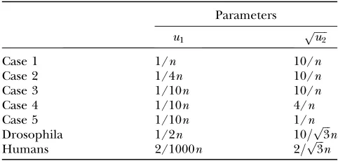
Let n ¼ 2N. Since our aim is to show that the theoretical predictions work well even for small values ofn, we will, in most cases, consider the valuesn¼1000 and n ¼ 10,000. Table 1 gives the seven simulation scenarios we study. Table 2 compares the predicted mean time from Theorem 1 with the average time found in 10,000 replications of each simulation. In making predictions for the examples, we consider that any numbersa andb satisfy a>b if a/b# 1/10. In case 3 our assumption 1= ffiffiffiffiffiu2
p
>n>1=u1 (Equation 1) about intermediate population size holds, and we can see that the simulated mean is very close to the predicted mean. In cases 1 and 5, we replace the upper and lower in-equalities in (1) by equality, respectively, so in each case one of the two assumptions is not valid. Cases 2 and 4 are intermediate, meaning that the upper and lower in-equalities in (1), respectively, do not quite hold since
the ratios are 1/4. Yet, cases 2 and 4 show good agreement with the predicted mean.
The last two cases are specific examples related to regulatory sequence evolution in Drosophila and hu-mans, which we consider in more detail in the next section. The Drosophila effective population size is too large to use the true value in the simulations, but this is feasible for humans. In addition, we multiplyu2by13 for these special cases so that the ratio u1/u2 ¼30. This comes from our assumption that a mutation at any position in the binding site will damage it, but to create a new binding site we require one position to mutate to the correct letter. Given a 10-letter target binding site, thenu1is 3310 times bigger thanu2.
In Figure 2, we plot the observed waiting time/ predicted mean for case 3 and see a good fit to the ex-ponential distribution, which agrees with our theoreti-cal prediction. Figure 3 corresponds to case 1 and shows that the tail of the distribution looks exponential, but the simulated mean time is 1.5 times larger than the predicted mean. This is caused by the fact that sinceu1¼ 1/(2N), the timetB–sBwe have to wait for theBmutant
to be produced is of the same order of magnitude assB.
Hence, the total waiting time tB is significantly larger thansB.
To explain the observed shape of the distribution, recall from the sketch of the proof of Theorem 1 thatsB
has exactly an exponential distribution. Adding the independent random variabletB–sB, which we assume
has densityg(s), yields the following distribution fortB, ðt
0
eðtsÞgðsÞds¼et
ðt
0
esgðsÞdstetgð0Þ whentis small
since the integrand is close tog(0) for alls2[0,t], and consequently the exponential fit is not good for smallt.
TABLE 1
Parameter values for our simulations in terms ofn¼2N
Parameters
u1 pffiffiffiffiffiu2
Case 1 1/n 10/n
Case 2 1/4n 10/n
Case 3 1/10n 10/n
Case 4 1/10n 4/n
Case 5 1/10n 1/n
Drosophila 1/2n 10=pffiffiffi3n
Humans 2/1000n 2=pffiffiffi3n
TABLE 2
Comparison of mean waiting times
Population size
Predicted mean
Simulated mean
Simulated/ predicted
Case 1 1,000 100 156.5 1.565
10,000 1,000 1,559 1.559
Case 2 1,000 400 460.0 1.150
10,000 4,000 4,552 1.138
Case 3 1,000 1,000 1,047 1.048
10,000 10,000 10,414 1.041
Case 4 1,000 2,500 2,492 0.997
10,000 25,000 2,5271 1.011
Case 5 1,000 10,000 7,811 0.781
10,000 100,000 77,692 0.777
Drosophila 1,000 346.4 441.1 1.273
10,000 3,464 4,374 1.263
Humans 20,000 8,660,258 6,464,920 0.747
Mean waiting times forn¼1000 andn¼10,000 are shown with mutation ratesu1and u2 as defined by each case. The simulated mean time is compared with the predicted mean from Theorem 1 and the ratio is given in the last column. All simulations are done with 10,000 replications.
Figure2.—Waiting time for case 3 withn¼1000 andu1¼
Wodarz and Komarova (2005) have done an exact
calculation of the waiting time in the branching process approximation of the Moran model, which applies to case 1. As Figure 3 shows, the computation matches the Moran model simulation exceptionally well.
Figure 4 corresponds to case 5 and yields a simulated mean of78% of its predicted value. The curve looks exponential, but it has the incorrect mean. In this case, Theorem 3 shows that fixation of anA mutation and stochastic tunneling are both possible scenarios in which a B mutation can arise, producing a shorter waiting time. More specifically, the assumptions of Theorem 3 hold with g ¼ 1, which gives a ¼ 1.433, and Figure 4 shows that the exponential distribution with this rate fits the simulated data reasonably well.
EXPERIMENTAL RESULTS
In the following two examples, we consider a 10-nucleotide binding site and suppose that transcription factor binding requires an exact match to its target. We assume that any mutation within the binding site will damage it (A mutation) and that at least one 10-nucleotide sequence exists within the regulatory region that can be promoted to a new binding site by one mutation (B mutation). Our previous results show, as MacArthurand Brookfield(2004) observed earlier,
that the existence of these so-called ‘‘presites’’ is necessary for the evolution of new binding sites on a reasonable timescale (Durrettand Schmidt2007).
Drosophila: We assume a per nucleotide mutation rate of 108
per generation, a simplification of the values that can be found in the classic article of Drakeet al.
(1998) and the recent direct measurements of Haag
-Liautard et al.(2007). If transcription factor binding
involves an exact match to a 10-nucleotide target, then inactivating mutations have probabilityu1¼107and those that create a new binding site from a 10-letter word that does not match the target in one position have probability u2 ¼ 13 3 108. If the target word is 6–9 nucleotides long or inexact matches are possible, then these numbers may change by a factor of 2 or 3. Such details are not very important here, since our aim is to identify the order of magnitude of the waiting time.
We set the effective population size N ¼2.5 3 106, which agrees with the value given on p. 1612 of Thorntonand Andolfatto(2006). To apply Theorem
1 we need
1=pffiffiffiffiffiu2 ¼1:733104>2N ¼53106>1=u1 ¼107: The ratio of the left number to the middle number1/ 300, but the ratio of the middle number to the one on the right is 1/2, which says that 2N>1=u1is not a valid assumption. Ignoring this for a moment, Theorem 1 predicts a mean waiting time of
1 2Nu1pffiffiffiffiffiu2 ¼
1:73 5 310
6171434;600 generations; which translates into 3460 years if we assume 10 generations per year.
Since the assumption 2N>1=u1 is not valid, we use our simulation result for case 6, which has a small population size with parameter values of 2Nu1¼0.5 and 2N ffiffiffiffiffiu2
p
¼10=pffiffiffi3¼5:77 similar to the Drosophila ex-ample, to see what sort of error we expect (see Tables 1 Figure 3.—Waiting time for case 1 withn¼ 1000, u1 ¼
0.001, andu2¼0.0001. The tail of the waiting-time distribu-tion appears to be exponential, but the simulated mean is
1.5 times larger than predicted by Theorem 1. The thick curve corresponds to the waiting-time calculation done by Wodarzand Komarova(2005). This computation matches
our Moran model simulation exceptionally well.
Figure 4.—Waiting time for case 5 withn¼ 1000, u1 ¼
0.0001, and u2 ¼ 0.000001. The simulated mean is only
and 2). We see that in the simulation, the observed mean is 25% higher than the theoretical mean, so adding 25% to the prediction gives a mean waiting time of 4325 years.
A second and more important correction to our prediction is that Theorem 1 assumes that the A mutation is neutral and the B mutation is strongly advantageous. If we make the conservative assumption that the B mutation is neutral, then the fixation probabilityb ¼1/2N ¼2 3 107, and by Theorem 1 the waiting time increases by a factor of 1=pffiffiffib2200 to 9 million years. If the Bmutation is mildly advanta-geous,i.e.,s– 1¼104, thenb104and the waiting time increases by a factor of only 100 to 400,000 years.
If we assume thatAmutants have fitnessr,1 where 1r> ffiffiffiffiffiu2
p
¼5:783105, then Theorem 4 implies that the waiting time is not changed, but ifð1rÞ= ffiffiffiffiffiu2
p ¼r, then the waiting time is increased by a factor 2=ðpffiffiffiffiffiffiffiffiffiffiffiffiffir214rÞ rifris large. If we use the value of 1 –r¼104, the increase is roughly a factor of 2. From this we see that if both mutations are almost neutral (i.e., relative fitnessesr1 – 104ands11104), then the switch between two transcription factor binding sites can be done in,1 million years. This is consistent with the results for theeven-skipped stripe 2 enhancer men-tioned earlier.
Humans:We now show that two coordinated changes that turn off one regulatory sequence and turn on another without either mutant becoming fixed are unlikely to occur in the human population. We assume a mutation rate of 108, again see Drake
et al.(1998), and an effective population size ofN¼104because this makes the nucleotide diversity 4Nemclose to the obser-ved value of 0.1%. If we again assume that transcription factor binding involves an exact match to a 10-nucleo-tide target, then inactivating mutations have probability u1¼107, and those that create a new binding site from a 10-letter word that does not match the target in one position have probability u2 ¼ 3.3 3 109. For the assumptions of Theorem 1 to be valid we need
1=pffiffiffiffiffiu2 ¼1:733104>2N ¼23104>1=u1 ¼107: The ratio of the middle number to the one on the right is 1/500, but the ratio of the left number to the middle one1.
Ignoring for the moment that one of the assumptions is not satisfied, Theorem 1 predicts a mean waiting time of
1 2Nu1pffiffiffiffiffiu2 ¼
1:73 2 310
7¼8:663106generations:
Multiplying by 25 years per generation gives 216 million years.
As shown in Tables 1 and 2, we have simulation results for humans using the exact parameters above. In 10,000 re-plications, the simulation mean is 6.46 million generations,
which is only75% of the predicted value. Multiplying by 0.75 reduces the mean waiting time to 162 million years, still a very long time. Our previous work has shown that, in humans, a new transcription factor binding site can be created by a single mutation in an average of 60,000 years, but, as our new results show, a coordinated pair of mutations that first inactivates a binding site and then creates a new one is very unlikely to occur on a reasonable timescale.
To be precise, the last argument shows that it takes a long time to wait for two prespecified mutations with the indicated probabilities. The probability of a seven of eight match to a specified eight-letter word is 8(3/4)(1/ 4)73.73 104, so in a 1-kb stretch of DNA there is likely to be only one such match. However, Lynch(2007,
see p. 805) notes that transcription factor binding sites can be found within a larger regulatory region (104– 106 bp) in humans. If one can search for the new target sequence in 104 – 106 bp, then there are many more chances. Indeed since (1/4)81.63105, then in 106bp we expect to find 16 copies of the eight-letter word.
The edge of evolution?Our final example of waiting for two mutations concerns the emergence of chloro-quine resistance in P. falciparum. Genetic studies have shown, see Wooton et al. (2002), that this is due to
changes in a protein PfCRT and that in the mutant strains two amino acid changes are almost always present—one switch at position 76 and another at position 220. This example plays a key role in the chapter titled ‘‘The mathematical limits of Darwinism’’ in Michael Behe’s book, The Edge of Evolution (Behe
2007).
Arguing that (i) there are 1 trillion parasitic cells in an infected person, (ii) there are 1 billion infected persons on the planet, and (ii) chloroquine resistance has arisen only 10 times in the past 50 years, he concludes that the odds of one parasite developing resistance to chloro-quine, an event he calls a chloroquine complexity cluster (CCC), are 1 in 1020. Ignoring the fact that humans
andP. falciparumhave different mutation rates, he then
concludes that ‘‘On the average, for humans to achieve a mutation like this by chance, we would have to wait a hundred million times ten million years’’ (Behe2007,
p. 61), which is 5 million times larger than the calcu-lation we have just given.
Indeed his error is much worse. To further sensation-alize his conclusion, he argues that ‘‘There are 5000 species of modern mammals. If each species had an average of a million members, and if a new generation appeared each year, and if this went on for two hundred million years, the likelihood of a single CCC appearing in the whole bunch over that entire time would only be about 1 in 100’’ (Behe2007, p. 61). Taking 2N¼106and
m1¼m2¼109, Theorem 1 predicts a waiting time of 31.6 million generations for one prespecified pair of mutations in one species, with ffiffiffiffiffiu2
p
We are certainly not the first to have criticized Behe’s work. Lynch(2005) has written a rebuttal to Beheand
Snoke (2004), which is widely cited by proponents of
intelligent design (see the Wikipedia entry on Michael Behe). Behe and Snoke(2004) consider evolutionary
steps that require changes in two amino acids and argue that to become fixed in 108generations would require a population size of 109. One obvious problem with their analysis is that they do their calculations for N ¼ 1 individual, ignoring the population genetic effects that produce the factor of ffiffiffiffiffiu2
p
. Lynch (2005) also raises
other objections.
CONCLUSIONS
For population sizes and mutation rates appropriate for Drosophila, a pair of mutations can switch off one transcription factor binding site and activate another on a timescale of several million years, even when we make the conservative assumption that the second mutation is neutral. This theoretical result is consistent with the observation of rapid turnover of transcription factor binding sites in Drosophila and gives some insight into how these changes might have happened. Our results show that when two mutations with ratesu1andu2have occurred and
1=pffiffiffiffiffiu2>2N>1=u1;
then the first one will not have gone to fixation before the second mutation occurs, and indeedAmutants will never be more than a small fraction of the overall population. In this scenario, theAmutants with fitnessr are significantly deleterious if ð1rÞ= ffiffiffiffiffiu2
p
is large, a much less stringent condition than the usual condition that 2N(1 –r) is large. Also, the success probability of theBmutant is dictated by its fitness relative to the wild type rather than relative to theAmutant. This follows because the fraction of A mutants in the population is small when the B mutant arises, and hence most individuals are wild type at that time.
The very simple assumptions we have made about the nature of transcription factor binding and mutation processes are not crucial to our conclusions. Our results can be applied to more accurate models of binding site structure and mutation processes whenever one can estimate the probabilities u1 and u2. However, the assumption of a homogeneously mixing population of constant size is very important for our analysis. One obvious problem is that Drosophila populations un-dergo large seasonal fluctuations, providing more opportunities for mutation when the population size is large and a greater probability of fixation of an A mutation during the recurring bottlenecks. Thus, it is not clear that one can reduce to a constant size population or that the effective population size com-puted from the nucleotide diversity is the correct
number to use for the constant population size. A second problem is that in a subdivided population,A mutants may become fixed in one subpopulation, giving more opportunities for the production ofBmutants or perhaps leading to a speciation event. It is difficult to analyze these situations mathematically, but it seems that each of them would increase the rate at which changes occur. In any case one would need to find a mechanism that changes the answer by a significant factor to alter our qualitative conclusions.
We thank Eric Siggia for introducing us to these problems and for many helpful discussions and Jason Schweinsberg for his collaboration on related theoretical results. We are also grateful to Nadia Singh, Jeff Jensen, Yoav Gilad, and Sean Carroll who commented on previous drafts and to two referees (one anonymous and Michael Lynch) who helped to improve the presentation. Both authors were partially supported by a National Science Foundation/National Institutes of General Medical Sciences grant (DMS 0201037). R.D. is also partially supported by a grant from the probability program (DMS 0202935) at the National Science Foundation. D.S. was partially supported by a National Science Foundation graduate fellowship at Cornell and after graduation was a postdoc at the Institute for Mathematics and its Applications in Minnesota, 2007–2008.
LITERATURE CITED
Behe, M., 2007 The Edge of Evolution. The Search for the Limits of
Darwinism.Free Press, New York.
Behe, M., and D. W. Snoke, 2004 Simulating evolution by gene
duplication of protein features that require multiple amino acid residues. Protein Sci.13:2651–2664.
Carter, A. J. R., and G. P. Wagner, 2002 Evolution of functionally
conserved enhancers can be accelerated in large populations: a population-genetic model. Proc. R. Soc. Lond.269:953–960. Drake, J. W., B. Charlesworth, D. Charlesworth and J. F.
Crow, 1998 Rates of spontaneous mutation. Genetics 148:
1667–1686.
Durrett, R., and D. Schmidt, 2007 Waiting for regulatory sequences
to appear. Ann. Appl. Probab.17:1–32.
Durrett, R., D. Schmidtand J. Schweinsberg, 2008 A waiting
time problem arising from the study of multi-stage carcinogenesis. Ann. Appl. Probab. (in press).
Ewens, W. J., 2004 Mathematical Population Genetics, Ed. 2.
Springer-Verlag, New York.
Haag-Liautard, C., M. Dorris, X. Maside, S. Macskill, D. L.
Halligan et al., 2007 Direct estimation of per nucleotide
and genomic deleterious mutation rates in Drosophila. Nature
445:82–85.
Iwasa, Y., F. Michorand M. A. Nowak, 2004 Stochastic tunnels in
evolutionary dynamics. Genetics166:1571–1579.
Iwasa, Y., F. Michor, N. L. Komarovaand M. A. Nowak, 2005
Pop-ulation genetics of tumor suppressor genes. J. Theor. Biol.233:
15–23.
Kimura, M., 1985 The role of compensatory mutations in molecular
evolution. J. Genet.64:7–19.
Kimura, M., and T. Ohta, 1969 The average number of generations
until the fixation of a mutant gene in a finite population. Genet-ics61:763–771.
Komarova, N. L., A. Senguptaand M. A. Nowak, 2003
Mutation-selection networks of cancer initiation: tumor suppressor genes and chromosomal instability. J. Theor. Biol.223:433–450. Ludwig, M. Z., N. H. Pateland M. Kreitman, 1998 Functional
analysis of eve stripe 2 enhancer evolution in Drosophila: rules governing conservation and change. Development 125:
949–958.
Ludwig, M. Z., C. E. Bergman, N. H. Patel and M. Kreitman,
Ludwig, M. Z., A. Palsson, E. Alekseeva, C. E. Bergman, J. Nathan
et al., 2005 Functional evolution of acis-regulatory module. PLoS Biol.3:588–598.
Lynch, M., 2005 Simple evolutionary pathways to complex proteins.
Protein Sci.14:2217–2225.
Lynch, M., 2007 The evolution of genetic networks by non-adaptive
processes. Nat. Rev. Genet.8:803–813.
MacArthur, S., and J. F. Brookfield, 2004 Expected rates and
modes of evolution of enhancer sequences. Mol. Biol. Evol.
21:1064–1073.
Nowak, M. A., 2006 Evolutionary Dynamics: Exploring the Equations of
Life.Belknap Press, Cambridge, MA.
Stone, J. R., and G. A. Wray, 2001 Rapid evolution ofcis-regulatory
sequences via local point mutations. Mol. Biol. Evol.18:1764–1770.
Thornton, K., and P. Andolfatto, 2006 Approximate Bayesian
inference reveals evidence for a recent, severe bottleneck in a Netherlands population of Drosophila melanogaster. Genetics
172:1607–1619.
Wodarz, D., and N. L. Komarova, 2005 Computational Biology of
Can-cer: Lecture Notes and Mathematical Modeling.World Scientific Pub-lishing, Hackensack, NJ.
Wooton, J. C., A. Feng, M. T. Ferdig, R. A. Cooper, J. Muet al.,
2002 Genetic diversity and chloroquine selective sweeps in Plas-modium falciparum.Nature.418:320–323.