©
DOI: 10.1534/genetics.104.033233
The Role of Pedigree Information in Combined Linkage Disequilibrium
and Linkage Mapping of Quantitative Trait Loci in a
General Complex Pedigree
S. H. Lee
1and J. H. J. Van der Werf
School of Rural Science and Agriculture, University of New England, New South Wales 2351, Australia Manuscript received July 2, 2004
Accepted for publication September 20, 2004
ABSTRACT
Combined linkage disequilibrium and linkage (LDL) mapping can exploit historical as well as recent and observed recombinations in a recorded pedigree. We investigated the role of pedigree information in LDL mapping and the performance of LDL mapping in general complex pedigrees. We compared using complete and incomplete genotypic data, spanning 5 or 10 generations of known pedigree, and we used bi- or multiallelic markers that were positioned at 1- or 5-cM intervals. Analyses carried out with or without pedigree information were compared. Results were compared with linkage mapping in some of the data sets. Linkage mapping or LDL mapping with sparse marker spacing (ⵑ5 cM) gave a poorer mapping resolution without considering pedigree information compared to that with considering pedigree information. The difference was bigger in a pedigree of more generations. However, LDL mapping with closely linked markers (ⵑ1 cM) gave a much higher mapping resolution regardless of using pedigree information. This study shows that when marker spacing is dense and there is considerable linkage disequilibrium generated from historical recombinations between flanking markers and QTL, the loss of power due to ignoring pedigree information is negligible and mapping resolution is very high.
C
OMBINED linkage disequilibrium (LD) and link- process needed in (fine) mapping of QTL is to estimate age mapping has been implemented in a variance IBD probabilities on the basis of LD and other available component approach, and analysis of simulated as well information including observed marker data and pedi-as real data hpedi-as proven that genomic regions containing gree information. This could cause difficulties when pre-quantitative trait loci (QTL) could be narrowed down to dicting IBD in general pedigrees as genotype probabili-within a few centimorgans (MeuwissenandGoddard ties are hard to derive when pedigrees are complex and 2000;Faniret al. 2002;Grisartet al. 2002;Meuwissen there are many missing genotypic data.et al. 2002;LeeandVan der Werf2004). As LD map- Although the general pedigree structure with missing ping can take into account the great number of histori- data is very common, accuracy or efficiency of combined cal recombinations reflected by identity-by-descent (IBD) LD and linkage (LDL) mapping for this situation has probability between haplotypes, positioning QTL can not been reported. This is because there is no obvious be very precise even with a relatively small number of ani- method of pedigree analysis dealing with complex rela-mals (Meuwissen and Goddard2000). Lee and Van tionships and a large proportion of missing data for der Werf(2004) investigated the efficiency of LD map- multiple closely linked markers. Exact methods for seg-ping in livestock using records of a few hundred progeny regation analysis such as pedigree peeling (Elstonand in a half-sib design and reported a high mapping reso- Stewart1971;Canningset al. 1978) or chromosome lution with confidence intervals up to just a few centi- peeling (LanderandGreen1987) are well-known
algo-morgans. rithms for estimating genotype probabilities on the basis
However, it is noted that in general such a design
of pedigree. However, the first method increases expo-may not always be available. Rather, a general pedigree
nentially in computational complexity with the number structure is commonly available and often used for
map-of markers, and the latter becomes infeasible with a ping of QTL. A general pedigree structure can span
large proportion of missing data. several generations with complex relationships, and
an-The locus sampler (Kong1991;Heath1997) uses a cestors’ genotypes are often unavailable and the
num-modification of the peeling algorithm and is much more ber of genotyped progeny is not always enough to
de-efficient and flexible for multilocus problems in a com-duce parental genotypes (Haley1999). However, a key
plex pedigree. It computes genotype probabilities using all pedigree information subsequently at each locus, conditional on flanking loci. However, this algorithm
1Corresponding author: School of Rural Science and Agriculture,
UNE, Armidale, NSW 2351, Australia. E-mail: slee7@metz.une.edu.au requires that pedigrees must be peelable at each locus.
lation alleles. In generationt, one of the base alleles surviving Alternatively, Markov chain Monte Carlo (MCMC)
algo-with a frequency of⬎0.1 and⬍0.9 was randomly chosen and rithms have been used to estimate genotype
probabili-treated as favorable with effect ␣ compared to other QTL ties, updating latent variables at a single locus subse- alleles. From generationt⫹1 to generationt⫹4 ort⫹9, quently for each individual, which makes it possible to pedigree was recorded and polygenic values were simulated. The recorded pedigree had complex relationships between deal with complex relationships in a pedigree. Examples
individuals because of random mating and selection. The base of algorithms are single-site genotypic samplers (Lange
parameter for population size wasNe⫽100 (t⫽100), with andMattyhysse1989;Sheehanet al. 1989) or
single-Ne⫽200 (t⫽200) orNe⫽800 (t⫽800) as alternative values. site segregation indicator samplers (Thompson1994). In the multiallelic marker model (e.g., microsatellites), the However, the irreducibility of the Markov chain is not number of alleles assumed in each marker locus was four and base allele frequencies were all at 0.25. In the biallelic marker easily guaranteed in complex pedigree structures and
model (e.g., single-nucleotide polymorphisms), the number mixing problems also appear in using multiple marker
of alleles was two and starting allele frequencies were 0.5. The loci (ThompsonandHeath1999;Canningsand
Shee-marker alleles were mutated at a rate of 4⫻10⫺4per genera-han2002). The meiosis Gibbs sampler (Thompsonand tion (Dallas1992;WeberandWong1993;Ellegren1995). Heath1999) greatly improves mixing by updating seg- A mutated locus was changed between the two existing alleles for biallelic markers whereas a new allele was added for multi-regation indicators jointly for all marker loci. However,
allelic markers. this approach is limited to pedigrees of moderate size
The role of pedigree information was investigated in linkage (⬍1000) since many MCMC cycles are required for an
mapping and LDL mapping, respectively. Analyses were
car-analysis. ried out for a complex pedigree spanning either 5 generations
Unfortunately, it is currently infeasible to use all avail- (generationstⵑt⫹4) or 10 generations (tⵑt⫹ 9). IBD probabilities were estimated either considering all relation-able information for a large complex pedigree with
ships across the recorded pedigree or considering only rela-sparse genotypic data (CanningsandSheehan2002).
tionships in the last generation (i.e., the parents of the last One may not be able to use complex relationships, and
generation were treated as unrelated).
the loss of information can affect the accuracy of posi- For a fair comparison between results, phenotypic values were tioning QTL. However, LDL mapping, as mentioned ear- available only for 100 individuals in the last generation in all
cases. Phenotypic values for individuals were simulated as lier, can use historical recombinations. If mutation age
is high, e.g.,⬎ 100 generations, recorded pedigree of
y⫽ ⫹ ␣ ⫹u⫹e. (1)
a few generations may contribute little to the
informa-The population mean () was 100, values for polygenic effects tion for positioning QTL. In this situation, it is
worth-(u) were drawn fromN(0,A2u) with2
u⫽25 (Ais numerator while to investigate the decrease of accuracy of LDL
relationships among individuals calculated since generation mapping when ignoring pedigree information. Note t⫹1), and values for residuals (e) were fromN(0,2e) with that omitting some pedigree information makes analy- 2
e⫽50. The favorable QTL allele had an additive value of ses much easier and faster. 7 (␣0⫽0 and␣1⫽7) and variance of QTL (VQTL) ranged from 8.8 to 24.5, depending on QTL allele frequency (0.1ⵑ 0.9 The aim of this study is to investigate the role of
pedi-in this study), withVQTL⫽2p(1⫺p)␣2(FalconerandMackay gree information in LDL mapping with a general
com-1996). The frequency of 0.1ⵑ0.9 may be reasonable for a plex pedigree. LDL mapping is carried out for a complex QTL that was previously detected by linkage mapping ( Meu-pedigree spanning 5 or 10 generations considering all wissen and Goddard 2000), and loci with more extreme pedigree information or considering the pedigree infor- allelic frequencies would contribute little to genetic variation and thus would not be appealing candidates for gene-mapping mation only in the last generation (i.e., ancestors of all
studies (unless in the case of a rare disease). animals in the last generation are treated as being
un-Analysis of data sets:Mixed linear model for detecting QTL:A related). The power advantage of LDL over linkage alone vector of phenotypic observations simulated from (1) can be is shown. The efficiency of LDL mapping with various modeled as
levels of LD in relation to pedigree information is
inves-y⫽X ⫹Zu⫹Zq⫹e, (2) tigated. In addition, it is shown how to efficiently
inte-grate the case of a complex pedigree with incomplete whereyis a vector of phenotypic observations on the trait of interest,is a vector of fixed effects,uis a vector of random genotypic data (genotypes are available only for the
polygenic effects for each individual,qis a vector of random progeny in the last generation) using Gibbs sampling.
effects due to QTL, andeare residuals. The random effectsu, q, andeare assumed to be normally distributed with mean zero and variance2
u,2q, and2e.XandZare incidence matrices MATERIALS AND METHODS for the effects in, anduandq, respectively. From (2), the associated variance-covariance matrix of all observations (V) Simulation study:A population of sizeNewas simulated for for a given pedigree and marker genotype set is modeled as 10 marker loci and a QTL fortgenerations to generate LD
beyond recorded pedigree between QTL and flanking mark- V⫽ZAZ⬘2
u⫹Z GRM Z⬘2q ⫹R, (3) ers. In each generation, the number of male and female parents
wasNe/2 and their alleles were inherited to descendants on whereAis the numerator relationship matrix based on addi-tive genetic relationships, GRM is the genotype relationship the basis of Mendelian segregation using the gene-dropping
method (MacClueret al. 1986). Parents were randomly mated matrix whose elements are IBD probabilities between individu-als computed for a putative QTL position and conditional on with a total of two offspring for each ofNe/2 mating pairs.
For the QTL, unique numbers were assigned to the base popu- marker information, andR⫽I2
Since the value of IBD probabilities between animals depends indicators of the flanking marker loci (Kong1991). The sam-pled genotypic configurations at the locus are converted to on the putative QTL position within a tested chromosome
re-gion, a number of different GRMs are generated. In this study, segregation indicators for sampling genotypic configuration we used 10 markers and tested QTL locations at the middle at the next marker locus. Therefore ordered genotypes and point of each marker bracket; therefore, nine GRMs were gen- segregation indicators are sampled across all individuals locus erated. Variance components for model parameters (2
u,2q, and by locus. The locus sampler has been implemented in MCMC
2e) were estimated with each GRM, using average information linkage software “LOKI” (Heath1997). We obtained one config-restricted maximum likelihood (AIREML;JohnsonandThomp- uration of the segregation indicators using LOKI in each
sam-son1995). The maximum values of the log likelihood for the pling round when using complete genotypic data or incom-different QTL locations were compared. plete genotypic data without parental relationships.
Gibbs sampling scheme for deriving IBD probabilities for GRM: Sampling segregation indicators by using the meiosis Gibbs sampler: With marker genotypes available for all individuals in the This algorithm makes joint updates for the inheritance of all recorded pedigree,i.e., parental and progeny’s genotypes are genes at linked loci, in a single meiosis. For example, for the known in each nuclear family, the correct linkage phase can mth meiosis, segregation indicators at all loci can be sampled often be assigned with a high certainty (MeuwissenandGod- using a forward-backward algorithm (ThompsonandHeath dard2000). Pong-Wonget al. (2001) reported that if ⬎10 1999), according to all possible segregation states for themth biallelic markers are used, the proportion of individuals having meiosis, conditional on the other meiosis (seeappendix). This at least one informative marker locus to assign correct phase sampler was used for incomplete genotypic data with all avail-is⬎90%. Therefore, the true set of haplotypes is close to the op- able relationships in a pedigree.
timal set of haplotypes estimated with the highest likelihood Haplotype reconstruction: Since LD-based IBD probabilities among all candidate sets of haplotypes. Therefore, we used are derived from haplotype similarity between unrelated base true haplotypes when using complete genotypic data (see also animals, ordered genotypes for base animals are required to
discussionand Table 2). However, when few genotypes are reconstruct haplotypes. The ordered genotypes can be sam-recorded on parents or further ancestors, there are many un- pled on the basis of the distribution of compatible allele assign-informative markers and many more possible sets of haplo- ments to founder genes that are consistent with the sampled types that can have similar likelihoods. For this case of using segregation indicators (Sobel andLange1996). When this incomplete genotypic data, all possible states of segregation procedure is implemented for multiple marker loci, haplo-need to be taken into account in an analysis. The meiosis types for base animals are established. This procedure is per-Gibbs sampler and the locus per-Gibbs sampler are considered formed in each sampling round.
to be suitable for this problem. Both samplers are supposed Initial legal configuration for the Markov chain:The meiosis to give the same result if they work properly. However, the Gibbs sampler requires a starting configuration, consistent with former is more efficient for sparse genotypic data (many miss- observed marker data, which is essential to start the Markov ing genotypes) while the latter is more efficient for dense chain.Heath(1998) used a combined method of pedigree genotypic data (few missing genotypes;Heath2003). As both peeling and a genotype elimination algorithm to sample geno-use segregation indicators as latent variables, the distribution type configurations, consistent with the observed marker data. of segregation indicators is described first, followed by a de- These can be converted to a legal configuration of segrega-scription of the sampling procedure. tion indicators. However, in the method, each locus should Distribution of segregation indicators given observed marker data: be peelable, which is not always guaranteed in the case of a One realization of segregation indicators (S) in a pedigree can complex pedigree with many missing genotypic data. Instead be expressed in anM⫻Lmatrix whose elements are 0 or 1. of using a peeling-based algorithm, the genotype elimination If the gene in themth meiosis at thelth locus receives the through inheritance constraint algorithm suggested by
Hen-paternal parental allele, the segregation indicatorSml⫽0, and shallet al. (2001) overcomes the problem of sampling for a Sml⫽1 for the maternal parental allele. The maximum number complex pedigree with genotypic data at a single locus. After of possible configurations for S is 2M⫻L when none of the the algorithm samples segregation indicators for each locus pedigree members are genotyped. The probability ofSgiven independently, the Gibbs procedure obtains the desired con-observed marker data is ditional distribution, taking into account the linkage between
markers.
IBD probabilities based on LD and linkage information:As ele-pr(S|G)⫽ pr(G|S)pr(S)
兺
pr(G|S)pr(S), (4) ments of GRM, IBD probabilities between all members are estimated on the basis of LD and linkage in each sampling whereGrepresents the observed marker data, pr(S) is prior round. Sampled haplotypes for base animals are used to esti-probability of the segregation indicators, pr(G|S) is the proba- mate LD-based IBD probabilities between unrelated base ani-bility of the observed marker data givenS, and the denomina- mals, using the method ofMeuwissenandGoddard(2000; tor is summed over the probabilities of all possible configura- 2001). Sampled segregation indicators at multiple loci for tions ofS. Since the computation of the denominator is not descendants are used to recursively estimate IBD probabilities feasible in general pedigrees, a Gibbs sampling scheme is between relatives given LD-based IBD probabilities of base required to obtain the posterior distribution of the segregation animals, using the method ofWanget al. (1995).indicators. A brief summary of the sampling procedure: Sampling segregation indicators by using the locus Gibbs sampler:
When pedigree is peelable at each marker locus (e.g., with few Do 1ⵑNcycles:
Sample segregation indicators for all meioses at all missing genotypic data with simple relationships), the locus
Gibbs sampler (Kong1991;Heath1997) can be used to ob- marker loci.
Sample haplotypes for base animals. tain segregation indicators and reconstructed haplotypes in
each sampling round. This method jointly updates the inheri- Estimate IBD based on sampled haplotypes and segrega-tion indicators.
tance of all genes for individuals (or meiosis), in a single locus.
Genotypic configurations are sampled from the distribution Construct GRM based on IBD. End do:
of genotype probabilities estimated by recursive peeling (
TABLE 1
Distribution of estimated QTL position
Deviation of estimated from correct position (cM)
Method ⫺4 ⫺3 ⫺2 ⫺1 0 1 2 3 4
5 generations with biallelic markers
LDLa-PEDb 5 4 6 18 28 15 14 3 7
LDL-NPEDc 3 4 10 16 26 18 15 4 4
L-PED 20 7 7 13 10 11 6 3 23
L-NPED 23 4 12 9 10 10 5 5 22
10 generations with biallelic markers
LDL-PED 11 4 7 14 28 14 9 6 7
LDL-NPED 10 5 4 18 27 14 11 2 9
L-PED 17 8 3 11 19 18 11 7 6
L-NPED 25 13 10 7 8 12 4 3 18
5 generations with multiallelic markers
LDL-PED 2 3 3 22 36 22 10 0 2
LDL-NPED 1 5 2 21 37 24 8 0 2
L-PED 15 9 12 10 11 11 10 7 15
L-NPED 28 2 4 6 9 6 11 9 25
10 generations with multiallelic markers
LDL-PED 5 3 5 16 43 20 4 3 1
LDL-NPED 6 2 3 17 42 18 4 4 4
L-PED 17 2 8 9 29 16 9 6 4
L-NPED 27 12 5 8 8 10 9 3 18
The estimated QTL position in 100 replicates with various mapping methods is shown.
aLDL, mapping using combined LD and linkage (L) information (linkage, using linkage only information). bPED, considering all pedigree information.
cNPED, considering only relationships between animals in the last generation.
Joint updates for the whole meiosis or the whole locus sam- the analysis considering all pedigree information (PED) pler result in better mixing properties and the process to be and the analysis ignoring relationships between individ-much more reliable than that of a single-site Gibbs sampler
uals until the last generation (NPED) for both 5 genera-(ThompsonandHeath1999). In addition, a sampler
updat-tions and 10 generaupdat-tions of pedigree. With the LDL ing segregation indicators rather than genotypic configuration
has a much smaller state space (Thompson1994). Therefore, method, the most frequently estimated position is in convergence of IBD probabilities could be reached quickly. the correct marker bracket and⬎55% of replicates posi-The Gibbs sampler was carried out for 5000 cycles, discarding
tion the QTL within 3 cM of the true position with the first 1000 cycles. In every tenth sampling round, elements
biallelic markers and⬎75% of replicates do the same of GRM were estimated and stored. They were averaged after
with multiallelic markers. the final sampling round. In the sampling procedure, allele
frequency at every marker locus was assumed equal (flat prior Linkage mapping alone:With linkage mapping, the ef-distribution). In each sampling round, it took ⵑ1.5 sec to fect of using pedigree information is large as the pattern obtain haplotypes and segregation indicators and ⵑ2.5 sec
of the distribution is quite different between PED and to estimate IBD probabilities in the pedigree spanning five
NPED. The difference is largest for the pedigree span-generations (CPU: 2.4 GHz).
ning 10 generations. Linkage mapping with biallelic markers and the pedigree spanning 5 generations most RESULTS frequently estimates the QTL position at the boundaries of the tested region with both PED and NPED, showing
Complete genotypic data: Distribution of the
esti-there is little information to position the QTL. A simi-mated position that deviated from the true QTL position
larly poor mapping resolution is obtained in the analysis in 100 replicates is illustrated in Table 1 for the case
for the pedigree spanning 10 generations with NPED, when all genotypic information is available on all
indi-but the QTL is more frequently positioned on the true viduals in the recorded pedigree (generation 100ⵑ104
position with PED;ⵑ45% of replicates position the QTL or 109).
within 3 cM of the true position (Table 1). In the multial-Combined LD and linkage mapping: In LDL mapping,
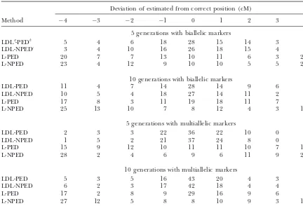
genera-Figure 1.—Pedigree spanning (A) 5 or (B) 10 generations. Likeli-hood ratio (LR) averaged over rep-licates in each putative position con-sidering all pedigree information (LDL-PED) and ignoring relation-ship between ancestors (LDL-NPED) and linkage mapping with pedigree information (L-PED) and no pedi-gree information (L-NPED) in the multiallelic marker model LR ⫽ 2(log LQTL ⫺ log Lno QTL). Solid diamond, LDL-PED; shaded box, LDL-NPED; solid triangle, L-PED; shaded dashed line, L-NPED.
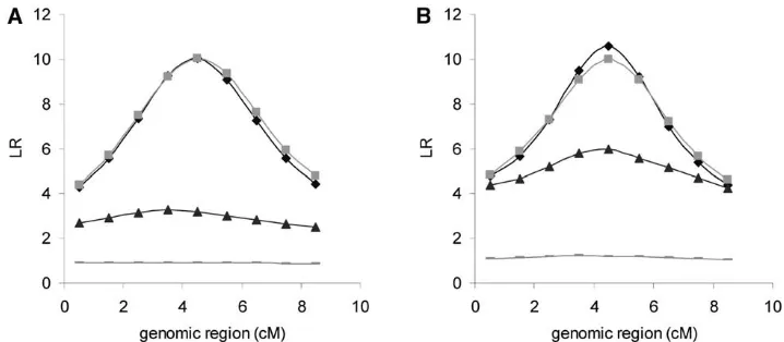
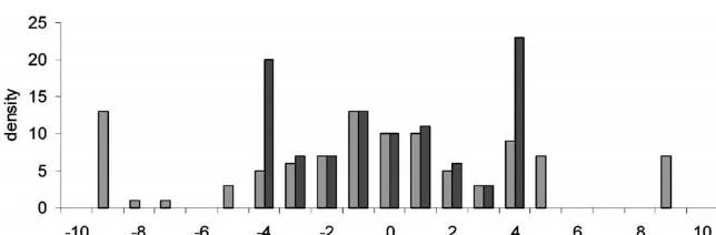
tions, the results are similarly poor as with biallelic mark- typic data, genotypes were available only for the progeny ers although PED positions the QTL in the correct in the last generation and all ancestral genotypes were marker bracket more frequently than NPED does. With missing. Figure 2 presents the distribution of estimated the pedigree spanning 10 generations, NPED gives poor QTL position deviated from the true location and the mapping resolution whereas PED frequently positions value of LR averaged over replicates when LDL mapping the QTL in the correct marker bracket;ⵑ50% of repli- is carried out with multiallelic markers and a pedigree cates position the QTL within 3 cM of the true position spanning five generations. The frequency of estimated
(Table 1). position near the correct QTL position is reasonably
The averaged likelihood ratio:The value of the likelihood high;⬎75% of replicates position the QTL within 3 cM ratio (LR) across the genomic region, averaged over of the true position. This result is similar to that with replicates with the multiallelic marker model, is plotted complete genotypic data. Although overall values of LR in Figure 1. The value of LR is almost flat in linkage are reduced compared to that with complete genotypic mapping with NPED in the pedigree of 5 generations data, there is an obvious peak, showing that there is (Figure 1A). Although the overall LR is higher in link- sufficient information to locate the QTL at the correct age mapping with PED, the difference between the high- position. As with complete genotypic data, the differ-est LR and lowdiffer-est LR is small, showing that not much ence between PED and NPED is not significant. information for positioning the QTL is provided by the The results with biallelic markers are similar to those pedigree spanning 5 generations. In the pedigree
span-with multiallelic markers in that the distribution of esti-ning 10 generations (Figure 1B), it is shown that linkage
mated QTL position is similar to that with complete mapping with NPED has no power to detect the QTL,
genotypic data, and the LR curve shows an obvious peak but linkage mapping with PED gives a considerably
at the true QTL position (results not shown). higher LR for the correct QTL position and there is an
The effect of marker density and past effective size
obvious peak, indicating much more information for
in relation to LD: Lower LD could arise from either positioning the QTL is provided when considering all
using a lower marker density or a higher effective popu-pedigree information compared with considering
rela-lation size. Figure 3 shows the pattern of LR values from tionships only in the last generation. This additional
in-LDL analyses averaged over replicates with 10 multial-formation from pedigree must account for the higher
lelic markers positioned at 5-cM intervals. The value of frequency of estimated QTL position in the correct marker
PED increases slightly with 5 generations of pedigree bracket in linkage mapping with PED compared with
and the increase is more significant for 10 generations NPED in the pedigree of 10 generations (Table 1).
of pedigree, compared to NPED. The value of LR with With LDL mapping, the LR curve is clearly peaked
NPED in each position is similar between 5 generations and highest at the correct QTL position, showing LDL
and 10 generations. When comparing with a marker mapping to be much more powerful than linkage
map-spacing of 1 cM, the LR values are much lower and the ping. In both pedigrees spanning 5 and 10 generations,
LR curve is flatter, indicating that LDL mapping with a it is also shown that the curves of LR in LDL mapping
sparse marker spacing does not give sufficient resolution with PED and NPED are similar, indicating that
pedi-(Figure 3). gree information is not so critical in LDL mapping
(Fig-Figure 4 shows LR values averaged over replicates ure 1).
whenNe⫽100, 200, or 800 for 100, 200, or 800 genera-The pattern of LR curves with biallelic markers is very
tions was simulated. The LR values were substantially similar to that with multiallelic markers although overall
decreased with higher values ofNeand results for PED LR values are lower (results not shown).
Figure 2.—Distribution of esti-mated QTL position deviated from the true QTL (A) and the value of LR averaged over replicates in each position (B) with the pedigree span-ning five generations in the multial-lelic marker model with incomplete genotypic data (genotypes are avail-able only for the animals in the last generation) using LDL mapping. (A) PED (lightly shaded bar), NPED (darkly shaded bar). (B) PED (solid triangle), NPED (shaded box).
The relationship between LD and the length of a broken up for 5 or 10 generations. This was the reason that with a lower LD, LDL mapping with PED gave chromosomal region that is IBD can be described as
higher accuracy than that with NPED in the marker spacing of 5 cM (Figure 3); however, the difference
be-LD ⫽ 1
1⫹4Nec ⫺2c⫺2Nec2⫹c2
(5)
tween PED and NPED was very small with a marker spacing of 1 cM (Figure 4).
(Svedand Feldman 1973), where Ne is past effective
Alternative QTL location: To test the performance size andcis the recombination rate of the chromosomal
of LDL mapping for QTL not centered in the studied region. LD is defined here as the probability of the
region, a QTL located at one-third of the tested region chromosomal region being IBD when two random
hap-was investigated. Figure 5 shows the distribution of esti-lotypes are taken from the population. The observed
mated QTL position and the value of LR averaged over value of LD based on simulated data agreed with the
replicates when LDL mapping is carried out with or expected value from (5). The averaged value of LD
without pedigree information. As in the case of a cen-observed over 100 replicates was 0.19⫾0.07 (expected
tered QTL, the frequency of estimated position as well value is 0.2) for a chromosome segment of 1 cM with
as the LR is highest at the correct QTL position and Ne⫽100. The value decreased to 0.04⫾0.01 (expected
the LR curve is fairly peaked. value is 0.05) for a segment of 5 cM withNe⫽100. Note
that the LR values were much lower with 5-cM marker intervals than with 1-cM intervals (Figure 3). The value
DISCUSSION also decreased with higher value ofNe,e.g., 0.11⫾0.04
(expected value is 0.11) and 0.03⫾0.01 (expected value While linkage mapping could greatly benefit from additional pedigree information, knowledge of relation-is 0.03) for a 1-cM segment with Ne ⫽ 200 and 800,
respectively. Note that the LR values were much lower ships between ancestors was not critical in LDL mapping with closely linked markers (ⵑ1 cM). The additional forNe⫽800 than forNe⫽100 (Figure 4). Given these
results, it is clearly shown that the levels of LD are closely information generated from the recorded relationship in a pedigree was very small compared to the LD infor-related to the efficiency of LDL mapping. With a lower
LD, pedigree information became useful if (and only mation generated from the historical population be-yond recorded pedigree. However, when using a lower if) the tested region was wide enough to be sufficiently
Figure4.—Pedigree spanning (A) 5 or (B) 10 generations. Values of LR averaged over replicates in each position for LDL mapping with vari-ous values of effective size when using complete genotypic data with multi-allelic markers. Solid diamond,Ne⫽ 100 with PED; shaded box,Ne⫽100 with NPED; solid triangle,Ne⫽200 with PED; shaded dashed line,Ne⫽ 200 with NPED; open circle,Ne⫽800 with PED; shaded circle, Ne ⫽ 800 with PED.
marker density (ⵑ5 cM), the degree of LD between correlations between parameters estimated with the true haplotypes and those with sampled haplotypes for 20 markers is much decreased and the recorded
relation-ships become more informative. In such cases, it is desir- replicates. For all variance components, the correlation between the two results is close to 1. Also for LR values able to use available pedigree information whenever
possible. at the true position, the results agreed very well. For the
estimated QTL position based on sampled haplotypes, When parental (ancestral) genotypes are absent, the
loss of information for positioning the QTL is small as 90–100% of replicates position the QTL within a dis-tance of one marker interval from the estimated QTL shown by the limited reduction of LR values in LDL
mapping with a 1-cM marker spacing;i.e., the most fre- position using true haplotypes for both 1- and 5-cM marker spacing. These results show that using true hap-quent estimated position was on the true QTL and the
LR curve was fairly peaked around the correct QTL lotypes is very similar to using sampled haplotypes in complete genotypic data.
position. This implies that parental haplotypes can be
reasonably well reconstructed from relatively few geno- Similar results were shown byMorriset al.(2004) in that the efficiency of fine mapping was not much re-types in the last generation in a general pedigree
(ap-proximately two to three progeny per family in our duced using a MCMC approach, compared with using the true haplotypes. The authors also showed that a study). These results agree with those ofAbecasiset al.
(2000), who reported that in the case that parental MCMC approach that considered all possible sets of haplotypes was much more efficient than inferring a set genotypes are missing, the loss of power for detecting
QTL is negligible when at least four genotyped progeny of haplotypes based on maximum likelihood. This was probably due to the fact that the likelihood was flat with per family are available. In our study, we used 10
mark-ers, which might help to assign linkage phase more respect to different haplotype configurations because no pedigree was used in deriving these haplotypes. Infer-correctly.
With complete genotypic data, we used true haplo- ring haplotypes in the case that parents’ and progeny’s genotypes and their relationships are fully known is types under the assumption that linkage phase is
as-signed with high certainty when parental and progeny expected to give better results, as was also shown by Pong-Wonget al.(2001).
genotypes are known. Results from true haplotypes and
those from sampled haplotypes were compared, using Since the locus sampler is based on a modification of the peeling algorithm that considers all compatible complete genotypic data spanning five generations with
a marker spacing of 1 or 5 cM. Table 2 shows high states simultaneously in a single locus, it does not have
TABLE 2 because the number of genotyped progeny per parent was low enough not to constrain parental allelic types. Correlation between parameters estimated with
Therefore, there were few or no noncommunicating true haplotypes and sampled haplotypes
classes in the Markov chain. Moreover, nearly identi-cal results from two very different MCMC approaches LR on the Positiona
2
␣ 2u 2P true QTL (%) proved the process to be reliable.
With sparse marker spacing (⬎5 cM) too wide to find 1-cM PED 1.00 1.00 1.00 0.99 100
LD information between QTL and flanking markers, it 1-cM NPED 0.98 1.00 1.00 1.00 100
is necessary to consider all pedigree information as the 5-cM PED 0.98 1.00 0.99 0.99 90
5-cM NPED 0.99 0.99 1.00 0.99 90 accuracy with PED and NPED was much different espe-cially in a deeper pedigree (Figure 3). The meiosis Gibbs Complete genotypic data spanning five generations with a
sampler can be an efficient tool to deal with complex marker spacing of 1 or 5 cM.
pedigree information in such cases. However, in some aProportion of replicates with sampled haplotypes
position-ing the QTL within one marker interval of estimated QTL data structures where allelic types of founders in a re-position with true haplotypes. corded pedigree are fully constrained by direct (if found-ers were genotyped) or indirect observations (foundfound-ers having a large number of genotyped progeny), the prob-lem of reducibility in the meiosis sampler would occur. reducibility problems (Heath 1997). However, its use
Block updating segregation indicators for a number of of computer memory requirement is too large to
oper-relatives simultaneously can be a way to increase irreduc-ate for a complex pedigree with a large proportion of
ibility although the large number of relatives can make missing genotypic data. The meiosis sampler is robust
it infeasible to compute genotype probabilities (i.e., the to complexity of pedigree and a large number of missing
number of segregation states is 22⫻nwithnthe number genotypes; however, when founder allelic types are
con-of individuals for which segregation indicators are strained, it can be reducible (Thompson and Heath
updated jointly). A random-walk approach (Sobeland 1999;Heath2003). Given the results from the analysis
Lange 1996) could be applied to noncommunicating based on the meiosis sampler (PED in Figure 2), there
classes using the Metropolis algorithm (Metropolis were no apparent problems of reducibility affecting the
et al. 1953). Further study is required to increase irreduc-results in our case. The pattern of distribution of
esti-ibility in the meiosis sampler. mated QTL position with PED, which was based on the
In linkage mapping especially with biallelic markers, meiosis sampler, was normal and similar to that with
the QTL was estimated more frequently at the bound-NPED, which was based on the locus sampler. The LR
aries than at the center in the tested region and the curve with PED was highly peaked at the true QTL
distribution of estimated positions did not seem normal position and the difference between highest and lowest
(Table 1). If the length of the tested region was in-position was significant. The pattern was similar to the
creased from 9 to 19 cM with the same data, estimated case of NPED. For a more reliable comparison, the
QTL positions were more normally distributed. Figure 6 accuracy and the values of LR with NPED were estimated
shows that the replicates positioning the QTL at the using the meiosis sampler and compared with those
boundaries in the tested region of 9 cM were actually based on the locus sampler. Ninety-four percent of
repli-the sum of repli-the estimates beyond this boundary. Probably cates with the meiosis sampler positioned the QTL
the most likely position was outside the tested region within 1 cM of that positioned on the basis of the locus
of 9 cM and the QTL was estimated at the boundary of sampler in LDL mapping. The correlation between
esti-the tested region that was closest to that point. It is ex-mated parameters based on the two samplers was 0.95
pected that the estimated positions would be completely for QTL variance, 0.98 for polygenic variance, and 0.99
normally distributed if the tested region is wide enough for phenotypic variance, and correlation between LR
values was 0.98. This similarity of results is probably (⬎ⵑ100 cM). Note that the distribution of estimated
position within⫺3 cM or 3 cM from the true position complex relationship with missing genotypic data could is very similar for either length of the tested regions. be efficiently integrated for fine mapping of QTL.
Similar results were observed in the study ofMeuwis- We are thankful for helpful discussion with Bruce Tier and Miguel senandGoddard (2000). When LD information was Perez-Enciso. Useful comments from reviewers are much appreciated. This study was supported by Australian Wool Innovation and a
Univer-reduced, the frequency of the estimated position
be-sity of New England research assistantship.
came higher at the boundaries. In the study ofSabry
et al.(2002), when LD information content was low, the proportion of replicates positioned at the boundaries
was much larger than that of those positioned in the LITERATURE CITED center regions. However, when there was more
informa-Abecasis, G. R., L. R. CardonandW. O. C. Cookson, 2000 A
tion, the estimated positions were normally distributed general test of association for quantitative traits in nuclear
fami-in a small region. lies. Am. J. Hum. Genet.66:279–292.
Bureau, A., 2001 Genetic linkage analysis based on identity by
de-Although the QTL effect was fixed, QTL heritability
scent using Markov chain Monte Carlo sampling on large
pedi-ranged from 0.11 to 0.25 because of different QTL allele grees. Ph.D. Thesis, University of California, Berkeley, CA. frequencies. However, the performance of mapping is Cannings, C., andN. A. Sheehan, 2002 On a misconception about
irreducibility of the single-site Gibbs sampler in a pedigree
appli-not substantially affected by QTL heritability unless
cation. Genetics162:993–996.
QTL allele frequency is extreme (⬍0.2 or ⬎0.8). The Cannings, C., E. A. ThompsonandM. H. Skolnick, 1978 Probabil-estimated position is similarly distributed near the cor- ity functions on complex pedigrees. Adv. Appl. Probab.10:26–61.
Dallas, J. F., 1992 Estimation of microsatellite mutation rates in
rect position for all values of heritability⬎0.15 (result
recombinant inbred strains of mouse. Mamm. Genome3:452–456.
not shown). This is because the QTL effect was constant Ellegren, H., 1995 Mutation rates at porcine microsatellite loci. and the effect as proportion of phenotypic SD was nearly Mamm. Genome6:376–377.
Elston, R. C., andJ. Stewart, 1971 A general model for the genetic
equal for all values of heritability (ranging from 0.7 to
analysis of pedigree data. Hum. Hered.21:523–542.
0.76). As shown byLeeandVan der Werf(2004), the
Falconer, D. S., and T. F. C.Mackay, 1996 Introduction to Quantita-accuracy substantially decreased with a lower pheno- tive Genetics, Ed. 4. Longman, Harlow/New York.
Fanir, F., B. Grisart, W. Coppieters, J. Riquet, P. Berziet al., 2002
typic SD (e.g.,⬍0.45P); however, as the number of records
Simultaneous mining of linkage and linkage disequilibrium to
used for fine mapping increased, the accuracy became
fine map quantitative trait loci in outbred half-sib pedigrees:
reasonably high. In this study, the number of records revisiting the location of a quantitative trait locus with major effect on milk production on bovine chromosome 14. Genetics
was only 100; therefore, the accuracy could easily be
161:275–287.
improved with a larger number of records.
Grisart, B., W. Coppieters, F. Fanir, L. Karim, C. Fordet al., 2002
Linkage disequilibrium between QTL and markers Positional candidate cloning of a QTL in dairy cattle: identifica-was generated from a large number of generations (in tion of a missence mutation in the bovineDGAT1gene with major effect on milk yield and composition. Genome Res.12:222–231.
this study,Ne ⫽ 100, 200, or 800 for 100, 200, or 800
Haley, C., 1999 Advances in quantitative trait locus mapping
(Ag-generations). A more correct simulation would simulate BiotechNet Proceedings 001 Paper 1), pp. 47–59 inFrom Jay Lush a number of background genes with a mutation model to Genomics: Visions For Animal Breeding and Genetics, edited by J. C. M.Dekkers, S. J.Lamontand M. F.Rothschild. Iowa
during the population history. However, it is arbitrary
State University, Ames, IA.
when deciding the number of background genes and Heath, S. C., 1997 Markov chain Monte Carlo segregation and their effect. Instead, we simply derived normally distrib- linkage analysis for oligogenic models. Am. J. Hum. Genet.61:
748–760.
uted polygenic effects for the last generation only,
as-Heath, S. C., 1998 Generating consistent genotypic configurations
suming the founders in the recorded pedigree were for multi-allelic loci and large complex pedigrees. Hum. Hered. unrelated. Since polygenic effects are not directly re- 48:1–11.
Heath, S. C., 2003 Genetic linkage analysis using Markov chain
lated to the efficiency of positioning QTL unless they are
Monte Carlo techniques, pp. 363–378 inHighly Structured Stochastic linked or there is epistasis, the assumption of unrelated
System, edited by P.Green, N. L. Hjortand S. Richardson.
founders when generating polygenic effects is not ex- Oxford University Press, Oxford.
Henshall, J. M., B. TierandR. J. Kerr, 2001 Estimating genotypes
pected to affect the main results.
with independently sampled descent graphs. Genet. Res.78:281–288.
In this study, generally, LDL mapping was much more
Johnson, D. L., andR. Thompson, 1995 Restricted maximum
likeli-powerful than linkage mapping alone in positioning the hood estimation of variance components for univariate animal QTL. If there were useful levels of LD (⬎ⵑ0.1), pedi- models using sparse matrix techniques and average information.
J. Dairy Sci.78:449–456.
gree information was not important. However, with
Kong, A., 1991 Analysis of pedigree data using methods combining
lower levels of LD due to sparser marker spacing, the peeling and Gibbs sampling. Computer Science and Statistics: efficiency of LDL mapping decreased and pedigree in- Proceedings of the Twenty-Third Symposium on the Interface. Interface Foundation of North America, Fairfax Station, VA,
formation became more informative. With higher
popu-pp. 379–385.
lation effective size, LD also decreases and a denser Lander, E. S., andP. Green, 1987 Construction of multilocus link-marker spacing is needed for LDL mapping to be effi- age maps in humans. Proc. Natl. Acad. Sci. USA84:2363–2367.
Lange, K., andS. Matthysse, 1989 Simulation of pedigree
geno-cient. Pedigree information will generally be less
infor-types by random walks. Am. J. Hum. Genet.45:959–970.
mative if the size of the region considered is too small
Lee, S. H., andJ. H. J. Van der Werf, 2004 The efficiency of designs
to allow sufficient recombinations during the recorded for fine-mapping of quantitative trait loci using combined linkage
disequilibrium and linkage. Genet. Sel. Evol.36:145–161.
MacCluer, J. W., J. L. VanderBerg, B. ReadandO. A. Ryder, 1986 of a variance component QTL fine mapping method. Proceedings of 7th World Congress on Genetics Applied to Livestock Production, Pedigree analysis by computer simulation. Zoo Biol.5:147–160.
August 19–23, Montpellier, France, Vol. 32, pp. 677–680.
Meuwissen, T. H. E., andM. E. Goddard, 2000 Fine scale mapping
Sheehan, N. A., A. Possolo and E. A. Thompson, 1989 Image of quantitative trait loci using linkage disequilibria with closely
processing procedures applied to the estimation of genotypes on linked marker loci. Genetics155:421–430.
pedigrees. Am. J. Hum. Genet.45(Suppl.): A248.
Meuwissen, T. H. E., andM. E. Goddard, 2001 Prediction of
iden-Sobel, E., andK. Lange, 1996 Descent graphs in pedigree analysis: tity by descent probabilities from marker-haplotypes. Genet. Sel.
application to haplotyping, location scores, and marker-sharing Evol.33:605–634.
statistics. Am. J. Hum. Genet.58:1323–1337.
Meuwissen, T. H. E., A. Karlsen, S. Lien, I. OlsakerandM. E.
Sved, J. A., andM. W. Feldman, 1973 Correlation and probability
Goddard, 2002 Fine mapping of a quantitative trait locus for
methods for one and two loci. Theor. Popul. Biol.4:129–132. twinning rate using combined linkage and linkage disequilibrium
Thompson, E. A., 1994 Monte Carlo likelihood in genetic mapping. mapping. Genetics161:373–379.
Stat. Sci.9:355–366.
Metropolis, N., A. Rosenbluth, M. Rosenbluth, A. Tellerand
Thompson, E. A., andS. C. Heath, 1999 Estimation of conditional
E. Teller, 1953 Equations of state calculation by fast computing
multilocus gene identity among relatives, pp. 95–113 inStatistics
machines. J. Chem. Phys.21:1087–1092.
in Molecular Biology and Genetics(IMS Lecture Notes), edited by
Morris, A. P., J. C. Whittaker andD. J. Balding, 2004 Little
F. Seller-Moiseiwitsch. Institute of Mathematical Statistics, loss information due to unknown phase for fine-scale linkage American Mathematical Society, Providence, RI.
disequilibrium mapping with single-nucleotide-polymorphism Wang, T., R. L. Fernando, S. Van der Beek, M. Grossmanand genotype data. Am. J. Hum. Genet.74:945–953. J. A. M. Van Arendonk, 1995 Covariance between relatives for
Pong-Wong, R., A. W. George, J. A. WoolliamsandC. S. Haley, a marked quantitative trait locus. Genet. Sel. Evol.27:251–274. 2001 A simple and rapid method for calculating identity- Weber, J. L., andC. Wong, 1993 Mutation of human short tandem by-descent matrices using multiple markers. Genet. Sel. Evol. repeats. Hum. Mol. Genet.2:1123–1128.
33:453–471.
Sabry, A., M. S. LundandB. Guldbrandtsen, 2002 Robustness Communicating editor: C. Haley
APPENDIX
Forward-backward algorithm in the meiosis sampler:FollowingThompsonandHeath (1999), we describe how to jointly sample segregation indicators of all genes at linked loci, in a single meiosis.
Forward working:In the forward working, the cumulative probability (Q) for the segregation indicatorSm,lis computed, conditional on all meioses at marker loci up to and including marker locus lexcept the mth meiosis itself, which is updating at the current stage. The working order is from the first marker to the last marker (1ⵑ L),
Ql(x)⫽pr(Sm,l⫽x|Sall⫺m,l,Gl,Sall⫺m,l*,Gl*), (A1)
wherex⫽ 0 (being transmitted from paternal) or 1 (from maternal),Sall⫺m,l ⫽all segregation indicators at locusl except the mth meiosis,Glis the observed marker data at locusl,Sall⫺m,l*is all segregation indicators from locus 1 to locus l⫺ 1 except themth meiosis, andGl*is the observed marker data from locus 1 tol⫺ 1.
The right-hand side in (A1) can be divided by two parts as
Ql(x)⫽ pr(Sm,l⫽ x|Sall⫺m,l,Gl)pr(Sm,l⫽x|Sall⫺m,l*,Gl*). (A2)
The first part in the right-hand side in (A2) can be obtained, using Bayes theorem:
pr(Sm,l ⫽x|Sall⫺m,l,Gl)⫽
pr(Gl|Sm,l⫽x,Sall⫺m,l)pr(Sm,l⫽x) 兺1
x⫽0pr(Gl|Sm,l ⫽x,Sall⫺m,l)pr(Sm,l⫽x)
. (A3)
pr(Sm,l⫽ x) is a prior probability with a value of 0.5; therefore, (A3) can be simplified as
pr(Sm,l ⫽x|Sall⫺m,l,Gl)⬀pr(Gl|Sm,l⫽ x,Sall⫺m,l). (A4)
The second part of the right-hand side in (A2) can be computed using the cumulative probability of the previous locus and recombination rate between locusland the previous locusl⫺1,
(Sm,l⫽ x|Sall⫺m,l*,Gl*)⬀Ql⫺1(x)(1⫺ l⫺1)⫹Ql⫺1(1⫺x)l⫺1, (A5)
wherel⫺1 is the recombination rate between the locuslandl⫺1. Note that for the first marker locus, the right-hand side in (A5) is negligible (⫽1) because there is no previous marker.
From (A1), (A4), and (A5),
Ql(x)⬀pr(Gl|Sm,l⫽ x,Sall⫺m,l){Ql⫺1(x)(1⫺ l⫺1)⫹Ql⫺1(1⫺ x)l⫺1}. (A6)
TABLE A1
Simple pedigree with genotypic data
Marker locia
IDb Sire Dam M1 M2 M3
1 0 0 0, 0 0, 0 0, 0
2 0 0 0, 0 0, 0 0, 0
3 1 2 1, 1 4, 1 3, 2
4 1 2 2, 2 4, 3 2, 2
aGenotypes are not ordered and 0 represents missing genotypes. bIdentification of animals.
QL(x)⫽ pr(Sm,L⫽x|Sall⫺m,L,GL,Sall⫺m,L*,GL*). (A7)
Therefore,Sm,Lcan be sampled from this posterior distribution.
Backward sampling: In backward sampling, the segregation indicator Sm,l is sampled conditional on the already sampled marker locus (Sm,l⫹1 ⵑ Sm,L) and using the cumulative probability for locus l that was computed in the forward working. The sampling order is the second last locus to the first locus (L⫺1ⵑ1):
pr(Sm,l ⫽x|Sall⫺m,l,Gl,Sall⫺m,l*,Gl*,Sm,l⫹1, . . . ,Sm,L)⬀Ql(x){|Sm,l⫹1⫺ x|l⫹(1 ⫺|Sm,l⫹1⫺x|)(1⫺ l)}. (A8)
A numerical example: Table A1 shows a simple pedigree with genotypic data for three markers (M1 ⵑ M3). Table A2 shows one legal configuration of segregation indicators in the pedigree as sampled in the first round. Joint updates for the third meioses (paternal gametes for animal 4 in italic letters) using the forward-backward algorithm are shown as an example. It is assumed that each marker has four alleles and allele frequencies are equal (0.25), and the recombination rate between each marker pair is 0.1.
The first term in the right-hand side in (A6) can be estimated for each marker locus using a descent graph:
pr(G1|S3,1⫽0,Sall⫺3,1)⫽ 0, pr(G1|S3,1⫽1,Sall⫺3,1)⫽ 0.0039 pr(G2|S3,2⫽0,Sall⫺3,2)⫽ 0.016, pr(G2|S3,2⫽1,Sall⫺3,2)⫽0.016 pr(G3|S3,3⫽0,Sall⫺3,3)⫽ 0.008, pr(G3|S3,3⫽1,Sall⫺3,3)⫽0.016.
For example, pr(G2|S3,2 ⫽ 1, Sall⫺3,2) is computed as follows. According to segregation indicators for the second marker, animal 3 has sire’s maternal gene (1M) and dam’s maternal gene (2M), and animal 4 has sire’s maternal gene (1M) and dam’s paternal gene (2P). Note that animals 3 and 4 are genotyped as (4, 1) and (4, 3), respectively. Therefore, the founder gene 1M, 2M, and 2P must be allele 4, 1, and 3 (no other allele assignment is possible). The probability of the allele assignment is the product of the frequencies of alleles involved in the allele assignment. Therefore, pr(G2|S3,2⫽1,Sall⫺3,2)⫽0.25 ⫻0.25⫻0.25⫽ 0.016.
The second term in the right-hand side in (A6) can be easily obtained using the cumulative probability for the previous locusl⫺1 and the recombination rate between locuslandl⫺1. For the first marker, the second term is negligible; therefore,Q1(0)⫽ 0 andQ1(1)⫽1. For the second marker,
Q2(0)⫽ 0.016{Q1(0)(1⫺ 1)⫹ Q1(1)1}
0.016{Q1(0)(1⫺ 1)⫹Q1(1)1}⫹0.016{Q1(1)(1 ⫺ 1)⫹Q1(0)1}
⫽ 0.1
Q2(1)⫽ 0.016{Q1(1)(1⫺ 1)⫹Q1(0)1}
0.016{Q1(0)(1⫺ 1)⫹ Q1(1)1}⫹0.016{Q1(1)(1 ⫺ 1)⫹Q1(0)1}⫽ 0.9.
For the last marker,
TABLE A2
Segregation indicators in the pedigree
ID Allele origin M1 M2 M3
3 Paternal 0 1 1
3 Maternal 1 1 1
4 Paternal 1 1 0
Q3(0)⫽ 0.008{Q2(0)(1⫺ 2)⫹Q2(1)2}
0.008{Q2(0)(1⫺ 2)⫹Q2(1)2}⫹0.016{Q2(1)(1⫺ 2)⫹ Q2(0)2}⫽0.099
Q3(1)⫽ 0.016{Q2(1)(1⫺ 2)⫹Q2(0)2}
0.008{Q2(0)(1⫺ 2)⫹Q2(1)2}⫹0.016{Q2(1)(1⫺ 2)⫹ Q2(0)2}
⫽0.901.
FromQ3, either 0 or 1 can be sampled forS3,3. Now let the value of 1 be sampled for the last locus. From (A8) in the backward sampling,
pr(S3,2⫽ 0|Sall⫺3,2,G2,Sall⫺3,2*,G2*,S3,3)⫽0.012, pr(S3,2⫽1|Sall⫺3,2,G2,Sall⫺3,2*,G2*,S3,3)⫽0.988.
Now, let the value of 1 be sampled for the second locus:
pr(S3,1⫽ 0|Sall⫺3,1,G1,S3,2,S3,3)⫽0, pr(S3,1⫽1|Sall⫺3,1,G1,S3,2,S3,3)⫽1.
The value of 1 is sampled for the first locus.