R E S E A R C H
Open Access
Hyperspectral imagery super-resolution by sparse
representation and spectral regularization
Yongqiang Zhao
*, Jinxiang Yang, Qingyong Zhang, Lin Song, Yongmei Cheng and Quan Pan
Abstract
For the instrument limitation and imperfect imaging optics, it is difficult to acquire high spatial resolution
hyperspectral imagery. Low spatial resolution will result in a lot of mixed pixels and greatly degrade the detection and recognition performance, affect the related application in civil and military fields. As a powerful statistical image modeling technique, sparse representation can be utilized to analyze the hyperspectral image efficiently. Hyperspectral imagery is intrinsically sparse in spatial and spectral domains, and image super-resolution quality largely depends on whether the prior knowledge is utilized properly. In this article, we propose a novel
hyperspectral imagery super-resolution method by utilizing the sparse representation and spectral mixing model. Based on the sparse representation model and hyperspectral image acquisition process model, small patches of hyperspectral observations from different wavelengths can be represented as weighted linear combinations of a small number of atoms in pre-trained dictionary. Then super-resolution is treated as a least squares problem with sparse constraints. To maintain the spectral consistency, we further introduce an adaptive regularization terms into the sparse representation framework by combining the linear spectrum mixing model. Extensive experiments validate that the proposed method achieves much better results.
Keywords:hyperspectral, sparse representation, super-resolution, linear mixing model
1. Introduction
Hyperspectral sensor can acquire imagery in many con-tiguous and very narrow (such as 10 nm) spectral bands that typically span the visible, near-infrared, and mid-infrared portions of the spectrum (0.4-2.5 μm) [1]. A continuous radiance spectrum for every pixel can be constructed from hyperspectral imagery, and it makes the identification of land-covers of interest possible based on their spectral signatures [1,2]. Hyperspectral remote sensing has widely been used for aerial and space imaging applications, including land use analysis, pollution monitoring, wide-area reconnaissance, and battle-field surveillance [3].
Although hyperspectral sensor can acquire higher spectral resolution information, for the instrument lim-itation and imperfect imaging optics, it is difficult to acquire high spatial resolution imagery. The spatial reso-lution is a key parameter in many applications related to space images (object detection and precise location to
name a few); it is obvious that any improvement here is important [3-5]. Low spatial resolution will result in a lot of mixed pixels and greatly degrade the detection and recognition performance, affect the related applica-tion in civil and military fields. There is significant sense to enhance the hyperspectral imagery’s spatial resolu-tion. In practice, modifying the imaging optics or the sensor array is not a good option, resolution enhance-ment using post-processing is a better way. Super-reso-lution image reconstruction offers the promise of overcoming the inherent resolution limitation of ima-ging sensors [4,5]. Conventional approaches to generat-ing a super-resolution image normally require as input multiple low-resolution image of the same scene, which are registered with sub-pixel accuracy [6]. But, it is diffi-cult for hyperspectral aerial and space remote sensing. Based on the hyperspectral imaging model [5], the super-resolution task is cast as the inverse problem of recovering the original high-resolution images, based on reasonable assumptions or prior knowledge about the observation model that maps the high-resolution image to the low-resolution ones [7]. For hyperspectral images, * Correspondence: [email protected]
College of Automation, Northwestern Polytechnical University, Xi’An 710072, China
the assumptions and prior knowledge are not only lim-ited to spatial domain, but also spectral domain. How to represent and utilize these assumptions and prior will affect the performance of super-resolution. For example, to ensure the spatial satisfaction of constraints, total var-iation (TV) model is used as prior to regularize the super-resolution problem [8]. Guo et al. [9] proposed a hyperspectral super-resolution algorithm using the spec-tral unmixing information and TV model. Based on the pixel neighborhood, the piecewise autoregressive (AR) models can be used to enhance the performance of restoration [10]. To get the better performance, the prior and assumption can be represented in Fourier-Wavelet domain [11].
As an emerging image modeling technique, sparse representation has successfully been used in various image super-resolution applications. The success of sparse representation owes to the development of l1
-norm optimization techniques, and the fact that natural images are intrinsically sparse in some domain [7]. Nat-ural images can be sparsely represented using a diction-ary of atoms, the dictiondiction-ary can be gotten through DCT/wavelet transforming or learning. It has been pro-ven that the sparsity of the coefficients can be served as good prior during the panchromatic image super-resolu-tion [7,12-15]. But, for hyperspectral image, the contents across different bands are related tightly. For hyperspec-tral image super-resolution, correlation among bands can be used as a prior, and more important thing is, after spatial super-resolution, the endmember of scene should not be changed. Based on these ideas, a novel hyperspectral image super-resolution method is pro-posed in this article. By analyzing the hyperspectral and panchromatic imaging process, we prove that dictionary learned from panchromatic images can be used to represent the hyperspectral images. Then the spectral mixing model is used to test the spectral consistency, and take it as a regularization term in super-resolution process. Finally, we present results obtained from experiments carried out on two datasets, namely a 118-band hyperspectral images captured under a controlled illumination laboratory environment and a 224-band air-borne visible/infrared imaging spectrometer (AVIRIS) image.
The rest of the article is organized as follows. Section 2 introduces the related works. Section 3 presents the super-resolution algorithm based on spatial sparsity and endmember regularization. Section 4 presents experi-mental results and Section 5 concludes the article.
2. Related studies
2.1. Sparse representation
It has been found that natural images can generally be coded by structured primitives, e.g., edges and line
segments [7], and these primitives are qualitatively simi-lar in form to simple cell receptive fields. Olshausen and Field [16] proposed to represent a natural image using a small number of basis functions chosen out of an over-complete code set. The sparse representation of a signal over an over-complete dictionary is achieved by optimiz-ing an objective function that includes two terms: one measures the signal reconstruction error and the other measures the signal sparsity.
Suppose that the data (image patch)x Î Rm admits a sparse approximation over an over-complete dictionary F ÎRn×m (K > m) withKatoms. Thenx can approxi-mately be represented as a linear combination of a few atoms from F. An over-complete dictionary Fand the sparse coefficientsa are obtained by solving the follow-ing optimization problem:
arg min
,α
x−α22+λα1 (1)
where ||·||2 is the 2 norm. For F, each of its atoms
(columns) is a unit vector in the l2 norm. They are
learned by solving the above minimization problem. l1
norm regularization constraint is used to guarantee the
sparseness of a, whereα1=
i |α
i|and a = [a1;...;
am]. Positive constantlcontrols the trade-off between accuracy of reconstruction and sparseness of a. The cost function given above is non-convex with respect to both Fanda. However, it is convex when one is fixed. Thus, this problem can be alternating between learning
F using K-SVD [17], MOD [18], or gradient descent
[19] while fixing a and inferringa using orthogonal matching pursuit (OMP) [20] while fixingF.
2.2. Hyperspectral and panchromatic images representation
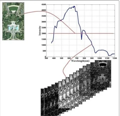
Hyperspectral imaging sensors divide the wavelength span (such as 0.4-1.2 μm) into a series of contiguous and narrow (such as 10 nm) spectral bands, and mea-sure the radiance of every bands. Panchromatic imaging sensors measure all the radiance in the wavelength spans (such as 0.4-1.2μm) once. For an arbitrary pixel in the hyperspectral or panchromatic image, digital number (or gray levels) of the image between wave-lengthl1and l2can be written as
DN= λ2
λ1 L(λ)Kigi(λ)dλ+B(λ1∼λ2) (2)
caused by dark signal. For same scene imaged by differ-ent sensors, L(l) is same. Figure 1 shows the principle of hyperspectral and panchromatic imaging processes.
Although image contents can vary a lot from image-to-image, it has been found that the micro-structures of images can be represented by a small number of struc-tural primitives (e.g., edges, line segments, and other ele-mentary features) [7]. Here, we can assume that spatial micro-structures information in hyperspectral bands can be derived from a series of panchromatic images. Based on this assumption, we can use the panchromatic
images to enhance the spatial resolution of hyperspectral images.
In sparse representation scheme, a natural image can be coded using a small number of basis functions cho-sen out of an over-complete code set. We can train the dictionaries using the patches extracted from sev-eral training panchromatic images which are rich in edges and textures. Here, we train two dictionaries using panchromatic image sets and hyperspectral image sets, as shown in Figures 2 and 3. The redun-dant DCT dictionary is described on the left side of
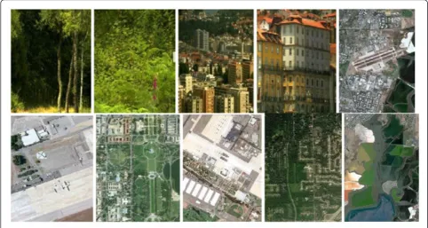
Figure 2, each of its atoms shown as an 8 × 8 pixel image. This dictionary was also used as the initializa-tion for all the training algorithms that follow. The globally trained dictionary is shown on the right side of Figure 2. This dictionary was produced by the K-SVD algorithm (executed 180 iterations, using OMP for sparse coding with), trained on a dataset of 1,00,000 8 × 8 patches. Those patches are taken from an arbitrary set of natural images (unrelated to the test images), some of which are shown in Figure 4.
3. Hyperspectral imagery super-resolution (HISR) with sparsity based regularization
HISR aims to reconstruct a high-quality imageryXfrom its degraded measurement Y. The hyperspectral imagery acquisition process can be modeled as:
Y =WHX+υ (3)
where Wrepresents the down-sampling operator and
Hrepresents a blurring filter, andυis the additive noise [2]. In this article, we just consider the spatial down-sampling and blurring operator. We can get the estima-tion of high-quality imagery Xˆ through resolving the inverse of (3):
ˆ
X= arg minY−WHX2
F (4)
where ||·||F is the F norm. The estimation of Xˆ by
formula (4) is a ill-posed inverse problem, since for a given low-resolution inputY, infinitely many high-reso-lution imagesX satisfy the reconstruction constraint. To find a better solution, prior knowledge of hyperspectral imagery can be used to regularize the HISR problem. We regularize the problem via the following prior on small patchxofX.
3.1. Spatial sparsity regularization
Panchromatic image is fused with hyperspectral image to enhance the spatial resolution, by extracting the structure information from a panchromatic image and injected into the hyperspectral image in a special
repre-sentation frame work. Here, we use a dictionary F =
[j1,...,jm]ÎRn×mtrained from high-resolution images to model the structure from panchromatic images. Based on this dictionaryF, the hyperspectral imagery acquisi-tion process can be modeled as
Y ≈WH+υ (5)
whereΛ= [a1;...;am] is them×Nmatrix where most of the elements inai(i= 1, 2,...,m) are close to zero.
ˆ
= arg min α
Y−WH2F+λ1 (6)
Λ = [a1, a2,...,aN] whereN is the number of band. That is fornth band, we have
ˆ
αn= arg min
αn
y−whφαn22+λαn1 (7)
3.2. Spectral regularization
Solving (7) individually for each band does not guaran-tee the compatibility between adjacent bands. We enforce compatibility between adjacent bands using the spectral regularization. For each given pixel, a linear spectral mixing model can be used to regularize the solution space, which is very helpful in preserving spec-tral consistency and suppressing noise. Let {mi}1≤i≤N
denote the set of Nendmember material signals. We
will arrange the signals mi as the columns of the
end-member matrixM. aiis the abundance of endmember
mi, and it satisfies the two constraints: non-negative and normality. We will write the abundance valuesa1,...,aN
Figure 2Left: Overcomplete DCT dictionary. Right: Globally trained dictionary.
as a column vector a. For mathematical simplicity, it is common to assume a linear mixing model:
f =Ma+n (8)
where f is the given spectral signal, n is the noise. The most straightforward approach for solving the lin-ear problem (8) is by constrained least squares minimi-zation
arg min
a xi−Ma 2
2 subject to ai>0,
i
ai= 1(9)
By incorporating the non-local similarity regularization term into the sparse representation, we have
ˆ
αn= arg min
αn
y−whφαn22+λαn1+γ
xi∈x
xi,n−Ma22
(10)
wheregis a constant balancing the contribution of the spectral regularization term. For a small patch, we write
the third term
xi∈x
xi,n−Ma22 as (I−B)φαn2 2,
whereIis the identity matrix and
B(i,j) =
Mai, ifxjis an element ofa
0, otherwise (11)
Then, formula (10) can be rewritten as
ˆ αn= arg minα
n
(f) = arg min
αn
y−whφαn22+λαn1+γ(I−B)φαn22
(12)
By letting
˜
y= y 0
, L= wh γ(I−B)
Formula (12) can be rewritten as
ˆ
αn= arg min
αn
˜y−Lφαn22+λαn1 (13)
This is a reweighted l1-minimization problem, which
can effectively be solved by the iterative shrinkage algo-rithm [21].
4. Experiment results and analysis
To test the performance of the super-resolution recon-struction algorithm, two kinds of experiments are designed. In the first experiment, the proposed super-resolution algorithm is tested on data which is collected under controlled illumination. The spectral span of images used for training and testing is same in this scene. In the second experiment, the algorithm is tested on the AVIRIS hyperspectral datasets. The super-resolu-tion results by proposed algorithm are compared with interpolation technique and hyperspectral super-resolu-tion method using endmember-based TV model [9].
4.1. Evaluation measures
The most common measure to quantitatively under-stand the performance of the reconstruction is the
signal-to-noise-ratio (PSNR). The peak signal value for each band can significantly change, which makes this measure biased toward bands with higher energy. To compensate this PSNR, the definition of standard is changed as follows
PSNR = 20 log
⎛ ⎜ ⎜ ⎜ ⎝
K
b=1
Speak,b √
MSE
⎞ ⎟ ⎟ ⎟
⎠ (14)
where Speak,bis the peak signal value at b’th band,
MSE is the mean square error between the ground truth and the estimated high-resolution signal.
Wang et al. [22] proposed a structural similarity mea-sure SSIM for two panchromatic images. For hyperspec-tral images, the means and variance should be vector.
The SSIM index between hyperspectral images x andy
can be defined as [22]
SSIM(x,y) = (2μ
T
xμy+C1)(2σxy+C2)
(μT
xμx+μTyμy+C1)(σTxσx+σTyσy+C2) (15)
Zhang et al [23] proposed a novel feature-similarity (FSIM) index for full reference image quality assessment. The phase congruency (PC) and gradient magnitude (GM) are utilized jointly in evaluating process. The
SSIM index between hyperspectral imagesx and ycan
be defined as [9]
FSIM(x,y) =
z∈
SL(z)·PCm(z)
z∈PCm(z)
(16)
whereΩ means the whole image spatial domain.PCm (z) = max{PCx(z), PCy(z)}, wherePCx(z) is phase con-gruency for a given position zof imagex. SL (z) is the gradient magnitude for a given positionz.
4.2. Indoor experiments
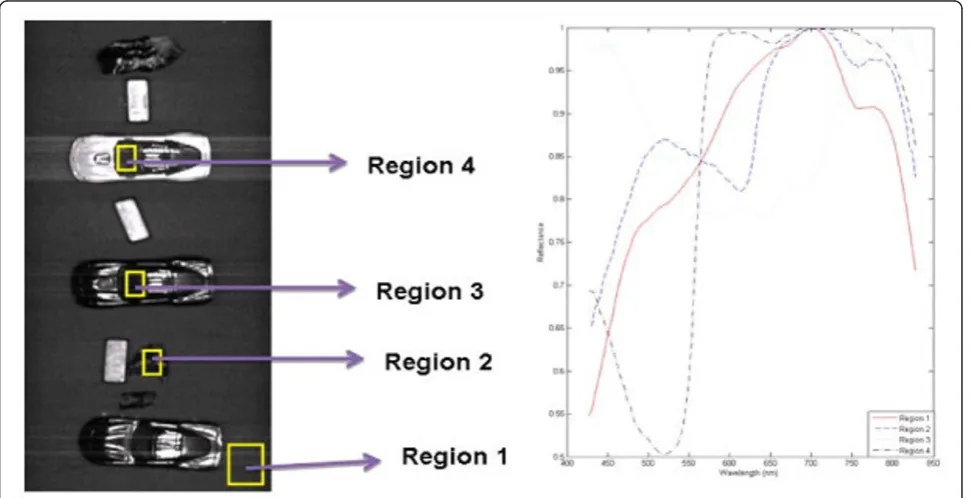
The data used in this experiment are the hyperspectral image captured at Instrumentation and Sensing Labora-tory (ISL) at Beltsville Agricultural Research Center (16 bit BIL, 307 rows by 307 columns by 118 bands, wave-length range: 426.9-853.0 nm, bandwidth: 4 nm) under control illumination. The spectral range of panchromatic images used to train the dictionary is 400-900 nm. Part of these panchromatic images comes from website [24], and some panchromatic images come from GoogleEarth, and some captured by our research group using Retiga EXi camera [25]. Figure 5 shows one scene and its cor-responding spectral reflectance.
In this experiment, the original ISL hyperspectral data are first down sampled by the nearest neighboring filter, band-by-band. Then, the linear spectral unmixing is per-formed on the down-sampled images. Here, a
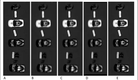
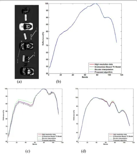
based N_FINDR algorithm is adopted for automatic extraction of endmembers. The details about this algo-rithm can be found in [26]. Figure 6 shows the super-resolution results by bicubic interpolation, endmember-based TV model, and proposed algorithm, and its corre-sponding PSNR, SSIM, and FSIM. By analyzing the images and evaluation measures in Figure 6, we can conclude that the proposed algorithm can get better PSNR and maintain more structure information. Figure 7 shows the spectral difference by different algorithm at different regions. Region 1 is smooth background, three different algorithms acquire almost same reflectance. Region 2 is edge, there is sharp variation of texture in this region, and only proposed algorithm can acquire almost same reflectance with original high-resolution data. The reflectance acquired by endmember-based TV model is obviously deviated from original high-resolu-tion data, and the reflectance error of bicubic interpola-tion is large. Region 3 is relative smooth edge region, and the reflectance difference is not so obvious. But, there is still obvious deviation of reflectance acquired by bicubic interpolation. The pre-trained dictionary has the adaptivity to image local structure, and the spectral reg-ularization can maintain the spectral information very
well. Although endmember information is used in end-member-based TV model, poor performance is acquired at edge region. Since the TV model favors the piecewise constant image structures, it tends to smooth out the fine details of an image.
5. Outdoor experiments
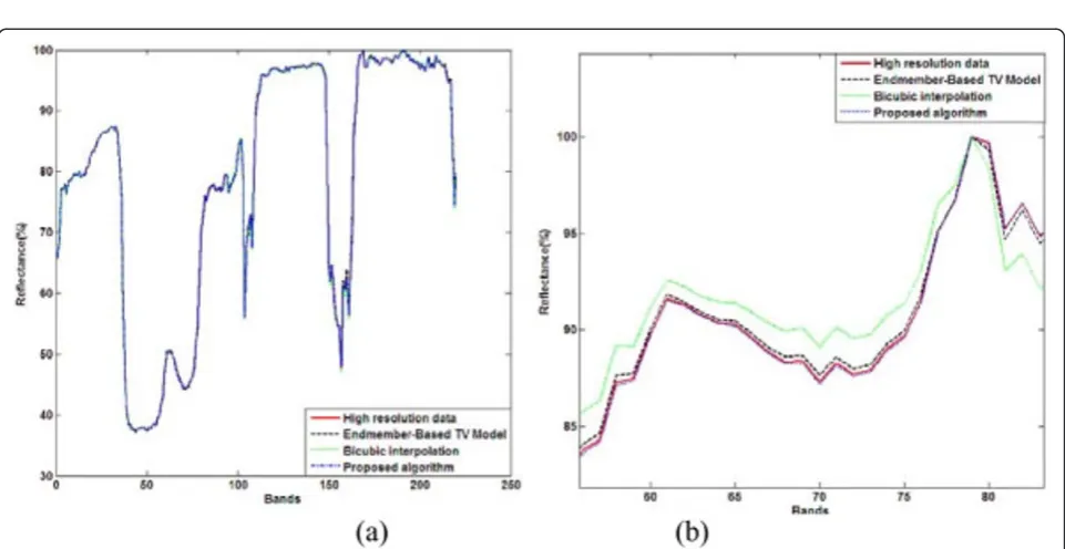
The dataset used in this experiment is the hyperspectral image of the Indian Pines (200 spectral bands in the 400-2500 nm range, 145 × 145 pixels), obtained by the AVIRIS sensor. Here, two dictionaries are trained for super-resolution of this kind of data. The first dictionary is trained using the panchromatic image with spectral covering within 400-900 nm. The second dictionary is trained using the multispectral images with spectral cov-ering within 400-2400 nm. The data used in second dic-tionary training come from different remote sensing satellites, such as LANDSAT and SPOT. Figure 8 shows the super-resolution results by bicubic interpolation, endmember-based TV model, and proposed algorithm, and its corresponding PSNR, SSIM, and FSIM. The experiment results in Figure 8 also shown that the pro-posed algorithm can get better performance. To better illustrate the robustness of the proposed method to the
Figure 6The results for a 118-band indoor hyperspectral database.(a)The original high-resolution data at band 70,(b)low-resolution image of(a)(downsampled in the spatial domain by a factor of 3),(c)bicubic interpolation (PSNR = 12.10, SSIM = 0.343364, FSIM = 0.4745),(d)
training dataset, we train two dictionaries using pan-chromatic image sets and hyperspectral image sets, some of panchromatic images are shown in Figure 4. Figure 8e, f shows the super-resolution results by the proposed algorithm using different dictionaries. By
comparing Figure 8e, f, we can conclude that using the different dictionaries almost same super-resolution results can be get. It can be explained as two different dictionaries are trained from sufficient large training remote sensing images sets, and almost all
micro-Figure 7Spectral difference by different super-resolution algorithms.(a)Different region location,(b)spectral difference at region 1,(c)
Figure 8The results for a 220-band Indian Pines test site of the AVIRIS database.(a)The original high-resolution data at band 70,(b) low-resolution image of(a)(downsampled in the spatial domain by a factor of three),(c)bicubic interpolation (PSNR = 19.97, SSIM = 0.550082, FSIM = 0.5822),(d)super-resolution by endmember-based TV model (PSNR = 20.30, SSIM = 0.666734, FSIM = 0.6230),(e)super-resolution by the proposed algorithm using the first dictionary (PSNR = 23.17, SSIM = 0.760108, FSIM = 0.6730),(f)super-resolution by the proposed algorithm using the second dictionary (PSNR = 23.19, SSIM = 0.760148, FSIM = 0.6737).
structures in nature scene can be captured in these two dictionaries. It can be proved by Figures 2 and 3. Figure 9 shows the spectral difference by different algorithm. In smooth region, there are no land cover’s variations, three different algorithms acquire almost same reflec-tance. But for the regions with obvious land cover’s var-iations, only proposed algorithm can acquire the almost reflectance with original high-resolution data.
5. Conclusion
We propose a novel hyperspectral super-resolution algo-rithm by utilizing the sparse representation and spectral mixing model. Single hyperspectral image super-resolu-tion is typical ill-posed inverse problem, prior knowl-edge of data can be used to regularize the super-resolution problem. Considering the fact that the micro-structures of images can be represented as linear combi-nation of atoms in the pre-trained dictionaries, we uti-lize the sparsity of combination coefficient to solve the inverse problem. To further improve the spectral quality of reconstructed images, we introduced a spectral mix-ing model-based image restoration framework. Spectral mixing models were learned from the training dataset and were used to regularize the image local smoothness. The experimental results on two hyperspectral images showed that the proposed approach outperforms state-of-the-art methods in both PSNR, visual, and spectral quality.
Acknowledgements
This work was supported by the Natural Science Foundation of China under grants Nos. 61071172, 60602056, and 60634030, and the Aviation Science Funds 20105153022, Sciences Foundation of Northwestern Polytechnical University No. JC200941.
Competing interests
The authors declare that they have no competing interests.
Received: 31 March 2011 Accepted: 12 October 2011 Published: 12 October 2011
References
1. Y Gu, Y Zheng, J Zhang, Integration of spatial-spectral information for resolution enhancement in hyperspectral images. IEEE Trans Geosci Remote Sens.46(5), 1347–1357 (2008)
2. T Akgun, Y Altunbasak, RM Mersereau, Super-resolution reconstruction of hyperspectral images. IEEE Trans Image Process.14(11), 1860–1875 (2005) 3. Y Zhao, L Zhang, SG Kong, Band-subset-based clustering and fusion for
hyperspectral imagery classification. IEEE Trans Geosci Remote Sens.49(2), 747–756 (2011)
4. FA Mianji, Y Zhang, HK Sulehria, Super-resolution challenges in hyperspectral imagery. Inf Technol J.7(7), 1030–1036 (2008). doi:10.3923/ itj.2008.1030.1036
5. T Akgun, Y Altunbasak, RM Mersereau, Super-resolution reconstruction of hyperspectral images. IEEE Trans Image Process.14(11), 1860–1873 (2005) 6. M Choi, R Kim, M Nam, HO Kim, Fusion of multispectral and panchromatic
satellite images using the curvelet transform. IEEE Geosci Remote Sens Lett. 2(2), 136–139 (2005). doi:10.1109/LGRS.2005.845313
7. W Dong, L Zhang, G Shi, X Wu, Image deblurring and super-resolution by adaptive sparse domain selection and adaptive regularization. IEEE Trans Image Process.20(7), 1838–1857 (2011)
8. T Chan, S Esedoglu, F Park, A Yip, Recent development in total variation image restoration, inMathematical Models of Computer Vision, ed. by Paragios N, Chen Y, Faugeras O (Springer, New York, 2005) 9. Z Guo, T Wittman, S Osher, L1 unmixing and its application to
hyperspectral image enhancement, inProc SPIE Conference on Algorithms and Technologies for Multispectral, Hyperspectral, and Ultraspectral Imagery XV, Orlando, Florida, (April 2009)
10. K Minami, S Kawata, S Minami, Superresolution of Fourier transform spectra by autoregressive model fitting with singular value decomposition. Appl Optics.24(2), 162–167 (1985). doi:10.1364/AO.24.000162
11. MD Robinson, CA Toth, JY Lo, S Farsiu, Efficient Fourier-wavelet super-resolution. IEEE Trans Image Process.19(10), 2669–2681 (2010) 12. J Yang, J Wright, TS Huang, Y Ma, Image super-resolution via sparse
representation. IEEE Trans Image Process.19(11), 2861–2873 (2010) 13. W Dong, G Shi, L Zhang, X Wu, Super-resolution with nonlocal-regularized
sparse representation, inSPIE VCIP, 7744 (2010)
14. W Dong, L Zhang, G Shi, X Wu, Nonlocal-back-projection for adaptive image enlargement, inICIP(2009)
15. W Dong, L Zhang, G Shi, Centralized sparse representation for image restoration, inICCV(2011)
16. BA Olshausen, DJ Field, Emergence of simple-cell receptive field properties by learning a sparse code for natural images. Nature.381, 607–609 (1996). doi:10.1038/381607a0
17. M Aharon, M Elad, A Katz, Y Bruckstein, The K-SVD: an algorithm for designing of overcomplete dictionaries for sparse representations. IEEE Trans Signal Process.54(11), 4311–4322 (2006)
18. H Lee, A Battle, R Raina, YN Andrew, Efficient sparse coding algorithms, in NIPS.19, 801–808 (2007)
19. J Mairal, F Bach, J Ponce, G Sapiro, Online learning for matrix factorization and sparse coding. J Mach Learn Res.11(1), 19–60 (2010)
20. R Rubinstein, M Zibulevsky, M Elad, Efficient implementation of the k-svd algorithm using batch orthogonal matching pursuit. Technical Report - CS Technion (2008)
21. I Daubechies, M Defriese, C DeMol, An iterative thresholding algorithm for linear inverse problems with a sparsity constraint. Commun Pure Appl Math.57, 1413–1457 (2004). doi:10.1002/cpa.20042
22. Z Wang, AC Bovik, H Rahim Sheikh, EP Simoncelli, Image quality assessment: from error visibility to structural similarity. IEEE Trans Image Process.13(4), 600–612 (2004). doi:10.1109/TIP.2003.819861
23. L Zhang, L Zhang, X Mou, D Zhang, FSIM: a feature similarity index for image quality assessment. IEEE Trans Image Process (2011)
24. DH Foster, SMC Nascimento, K Amano, Information limits on neural identification of coloured surfaces in natural scenes. Visual Neurosci.21, 331–336 (2004). doi:10.1017/S0952523804213335
25. Y Zhao, P Gong, Q Pan, Object detection by spectropolarimeteric imagery fusion. IEEE Trans Geosci Remote Sens.46(10), 3337–3345 (2008) 26. A Plaza, P Martinez, R Perez, J Plaza, A quantitative and comparative analysis
of endmember extraction algorithm from hyperspectral data. IEEE Trans Geosci Remote Sens.42(3), 650–663 (2004). doi:10.1109/TGRS.2003.820314
doi:10.1186/1687-6180-2011-87
Cite this article as:Zhaoet al.:Hyperspectral imagery super-resolution by sparse representation and spectral regularization.EURASIP Journal on Advances in Signal Processing20112011:87.
Submit your manuscript to a
journal and benefi t from:
7Convenient online submission 7Rigorous peer review
7Immediate publication on acceptance 7Open access: articles freely available online 7High visibility within the fi eld
7Retaining the copyright to your article