Denoising algorithm for the 3D depth map sequences based on multihypothesis motion estimation

(1)

R E S E A R C H

Open Access

Denoising algorithm for the 3D depth map

sequences based on multihypothesis motion

estimation

Ljubomir Jovanov

*

, Aleksandra Pi

ž

urica and Wilfried Philips

Abstract

This article proposes an efficient wavelet-based depth video denoising approach based on a multihypothesis motion estimation aimed specifically at time-of-flight depth cameras. We first propose a novel bidirectional block matching search strategy, which uses information from the luminance as well as from the depth video sequence. Next, we present a new denoising technique based on weighted averaging and wavelet thresholding. Here we take into account the reliability of the estimated motion and the spatial variability of the noise standard deviation in both imaging modalities. The results demonstrate significantly improved performance over recently proposed depth sequence denoising methods and over state-of-the-art general video denoising methods applied to depth video sequences.

Keywords:3D capture, depth sequences, video restoration, video coding

1 Introduction

The impressive quality of user perception of multimedia content has become an important factor in the electro-nic entertainment industry. One of the hot topics in this area is 3D film and television. The future success of 3D TV crucially depends on practical techniques for the high-quality capturing of 3D content. Time-of-flight sensors [1-3] are a promising technology for this purpose.

Depth images also have other important applications in the assembly and inspection of industrial products, autonomous robots interacting with humans and real objects, intelligent transportation systems, biometric authentication and in biomedical imaging, where they have an important role in compensating for unwanted motion of patients during imaging. These applications require even better accuracy of depth imaging than in the case of 3D TV, since the successful operation of var-ious classification or motion analysis algorithms depends on the quality of input depth features.

One advantage of TOF depth sensors is that their suc-cessful operation is less dependent on a scene content

than for other depth acquisition methods, such as dis-parity estimation and structure from motion. Another advantage is that TOF sensors directly output depth measurements, whereas other techniques may estimate depth indirectly, using intensive and error-prone com-putations. TOF depth sensors can achieve real-time operation at quite high frame rates, e.g. 60 fps.

The main problems with the current TOF cameras are low resolution and rather high noise levels. These issues are related to the way the TOF sensors work. Most TOF sensors acquire depth information by emitting continuous-wave (CW) modulated infra-red light and measuring the phase difference between the sent (refer-ence) and received light signals. Since the modulation frequency of the emitted light is known, the measured phase directly corresponds to the time of flight, i.e., the distance to the camera.

However, TOF sensors suffer from some drawbacks that are inherent to phase measurement techniques. The first group of depth image quality enhancement meth-ods aims at correction of systematic errors of TOF sen-sors and correcting distortions due to non-ideal optical system, as in [4-7]. In this article, we address the most important problem related to TOF sensors, which limits the precision of depth measurements: signal dependent

* Correspondence: [email protected]

Ghent University-TELIN-IPI-IBBT Sint-Pietersnieuwstraat 41, B-9000 Gent, Belgium

(2)

noise. As shown in [1,8], noise variance in TOF depth sensors, among other factors, depends on the intensity of the emitted light, the reflectivity of the scene and the distance of the object in the scene.

A large number of methods have been proposed for spatio-temporal noise reduction in TOF images and similar imaging modalities, based on other 3D scanning techniques. Techniques based on non-local denoising [9,10] were applied to sequences acquired using the structured light methods. For a given spatial neighbour-hood, they find the most similar spatio-temporal neigh-bourhoods in other parts of the sequence (e.g., earlier frames) and then compute a weighted average of these neighbourhoods, thus achieving noise reduction. Other non-local techniques, specifically aimed at TOF cameras have been proposed in [8,11,12]. These techniques use luminance images as a guidance for non-local and cross-bilateral filtering. The authors of [12-14] present a non-local technique for simultaneous denoising and up-sampling of depth images.

In this article, we propose a new method for denoising depth image sequences, taking into account information from the associated luminance sequences. The first novelty is in our motion estimation, which takes into account information from both imaging modalities and accounts for spatially varying noise standard deviation. Moreover, we define reliability to this estimated motion and we adapt the strength of temporal denoising according to the motion estimation reliability. In parti-cular, we use motion reliabilities derived from both depth and luminance as weighting factors for motion compensated temporal filtering.

The use of luminance images brings us multiple bene-fits. First, the goal of existing non-local techniques is to find other similar observations in other parts of the depth sequence. However, in this article, we look for observations both similar in depth and luminance. The underlying idea here is to average multiple observations of the same object segments. As luminance images have many more textural features than depth images, the located matches can be better in quality, which improves the denoising. Moreover, the luminance image is less noisy, which facilitates the search for similar blocks. We have confirmed this experimentally by calcu-lating peak signal-to-noise ratio (PSNR) of depth and luminance measurements, using ground truth images obtained by temporal averaging of the 200 static frames. Typically, depth images acquired by SwissRanger camera have PSNR values of about 34-37 dB, while PSNR values of luminance are about 54-56 dB. Theoretical models from [15] also confirm that noise variance in depth is larger than noise variance in luminance images.

The article is organized as follows: In Section 2, we describe the noise properties of TOF sensors and a

method for generating the ground truth sequences, used in our experiments. In Section 3, we describe the pro-posed method. In Section 4, we compare the propro-posed method experimentally to various reference methods in terms of visual and numerical quality. Finally, Section 5 concludes the article.

2 Noise characteristics of TOF sensors

TOF cameras illuminate the scene by infra red light emitting diodes. The optical power of this modulated light source has to be chosen based on a compromise between image quality and eye safety; the larger the optical power, the more photoelectrons per pixel will be generated, and hence the higher the signal-to-noise ratio and therefore the accuracy of the range measurements. On the other hand, the power has to be limited to meet safety requirements. Due to the limited optical power, TOF depth images are rather noisy and therefore rela-tively inaccurate. Equally important is the influence of the different reflectivity of objects in the scene, which reduce the reflected optical power and increase the level of noise in the depth image. Interferences can also be caused by external sources of light and multiple reflec-tions from different surfaces.

As shown in [16,17], the noise variance and therefore the accuracy of the depth measurements depends on the amplitude of the received infra red signal as

L= √L 8·

√

B

2·A, (1)

where AandBare the amplitude of the reflected sig-nal and its offset, L the measured distance andΔLthe uncertainty on the depth measurement due to noise. As the equation shows, the noise variance, and therefore the depth accuracy ΔL is inversely proportional to the demodulation amplitudeA.

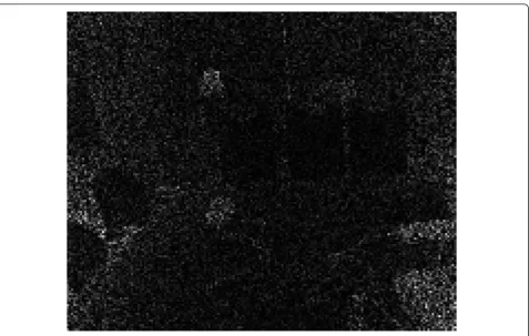
In terms of image processing, ΔL is proportional to the standard deviation of the noise in the depth images. Due to the inverse dependence of ΔAon the detected signal amplitudeAand the fact that Ais highly depen-dent on the reflectance and distance of objects, the noise variance in the depth scene is highly spatially vari-able. Another effect contributing to this variability is that the intensity of the infra-red source decreases with the distance from the optical axis of the source. Conse-quently, the depth noise variance is higher at the bor-ders of the image, as shown in Figure 1.

2.1 Generation a“noise-free”reference depth image

(3)

this is of limited use in dynamic scenes, we exploit this principle to generate an approximately noise free refer-ence depth sequrefer-ence of a static scene captured by a moving camera.

Each frame in the noise-free sequence is created as follows: the camera is kept static and 200 frames of the static scene are captured and temporally averaged. Then, the camera is moved slightly and the procedure is repeated, resulting in the second frame of the reference depth sequence. The result is an almost noise free sequence, simulating a static scene captured by a mov-ing camera. This way we simulate translational motion of the camera. If the reference “noise-free” depth sequence containsk frames,k× 200 frames should be recorded.

3 The proposed method

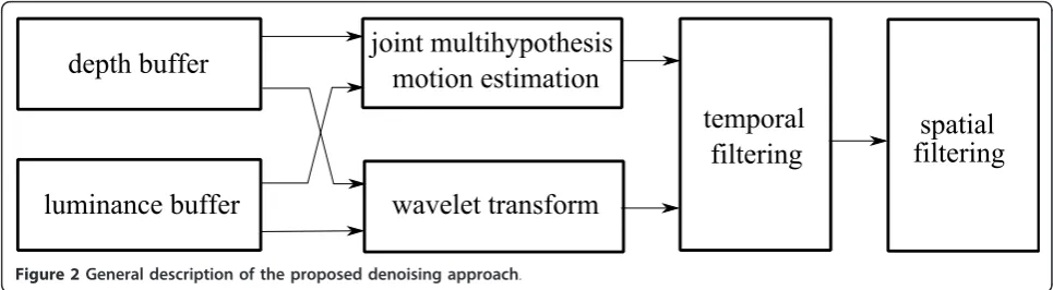
The proposed method is depicted schematically in Fig-ure 2. The proposed algorithm operates on a buffer which contains a given fixed number of depth and lumi-nance frames.

The main principle of the proposed multihypothesis motion estimation algorithm is shown in Figure 3. The motion estimation algorithm estimates the motion of blocks in the middle frame, F(t). The motion is determined relative to the framesF(t - k),...,

F(t- 1), F(t+ 1),..., F(t +k), where 2k + 1 is the size of the frame buffer. To achieve this, reference frameF (t) is divided into rectangle 8 × 8 pixels blocks. For each block in the frame F(t), a motion estimation algorithm searches neighbouring frames for a certain number of candidate blocks most resembling the cur-rent block fromF(t). For each of the candidate blocks, the motion estimation algorithm computes a reliability measure for the estimated motion. The idea of the uti-lization of motion estimation algorithms for collecting highly correlated 2D patches in a 3D volume and denoising in 3D transform domain was first intro-duced in [18]. A similar idea of multiframe motion compensated filtering, entirely in the pixel domain was first presented in [19].

The motion estimation step is followed by the wavelet decomposition step and by motion compensated filter-ing, which is performed in the wavelet domain, using a variable number of motion hypotheses (depending on their reliability) and data dependent weighted averaging. The weights used for temporal filtering are derived from the motion estimation reliabilities and from the noise standard deviation estimate. The remaining noise is removed using the spatial filter from [20], which oper-ates in wavelet domain and uses luminance to restore lost details in the corresponding depth image.

(4)

3.1 The multihypothesis motion estimation method

The most successful video denoising methods use both temporal and spatial correlation of pixel intensities to sup-press noise. Some of these methods are based on finding a number of good predictions for the currently denoised pixel in previous frames. Once found, these temporal pre-dictions, termed motion-compensated hypotheses are aver-aged with the current, noisy pixel itself to suppress noise.

Our proposed method exploits the temporal redun-dancy in depth video sequences. It also takes into account that a similar context is more easily located in the luminance than in the depth image.

Each frameF(t) in both the depth and the luminance is divided into 8 × 8 non-overlapping blocks. For each

block in the frameF(t), we perform a three-step search algorithm from [21] within some support regionVt-1.

The proposed motion estimation algorithm operates on a buffer containing multiple frames (typically 7). Instead of finding one best candidate that minimizes the given cost function, here we determineNcandidates in the frameF(t- 1) which yield theNlowest values of the cost function. Then, we continue with the motion esti-mation for each of the Nbest candidates found in the frame F(t - 1) by finding their N best matches in the frameF(t- 2). We continue the motion estimation this way until the end of the buffer is reached. This way, by only taking into account the areas that contain the blocks most similar to the current reference block, the

depth buffer

luminance buffer

joint multihypothesis

motion estimation

wavelet transform

temporal

filtering

spatial

filtering

Figure 2General description of the proposed denoising approach.

(5)

search space is significantly reduced, compared to a full search in every frame: instead of searching the area of 24 × 24 pixels in the frames F(t - 1) and F(t+ 1) and area of 40 × 40 pixels in the framesF(t- 2) andF(t+ 2) and ((24 + 2 × 8 × k) × (24 + 2 × 8 ×k) pixels in the framesF(t-k) andF(t+k), the search algorithm we use [21] is limited to the areas of 242Nc pixels, which brings

significant speed-ups. Formally, the set ofN-best motion vectors Vˆi is defined for each blockBiin the frameF(t)

as:

ˆ

Vi={ˆvn}n=1..N, (2)

where each motion vector candidate v_ˆn from the frameF(t-dt) is obtained by minimizing:

ri(vn) =

j∈Bi

|F(j,t)−F(j−vn,t−dt)|, ₍₃₎

wheredt≤Nf. In other words, for each blockBiin the

frame F(t) we search for the blocks in the framesF(t -Nf),...,F(t- 1),F(t+ 1),..., F(t+Nf) which maximize the

similarity measure between blocks.

Since the noise in depth images has a non-constant standard deviation, and some depth details are some-times masked by noise, estimating the motion based on depth only is not very reliable. However, the luminance image typically has a good PSNR and has a stationary noise characteristics. Therefore, in most cases we rely more on the luminance image, especially in areas where the depth image has poor PSNR. In the case of noisy depth video frames, we can write

f(l) =g(l) +n(l), (4)

where f(l),g(l) and n(l) are the vectors containing noisy, noise-free pixels and noise realizations at the location l, respectively. Each of these vectors contains pixels of both the depth and the luminance frame at spatial position l. We define the displaced frame differ-ence for each pixel inside blocksBiin the frames F(t),F

(t- 1) as

r(l,v(l),t) = [g(l−v(l),t−1)−g(l,t)]

+[n(l−v(l),t−1)−n(l,t)], (5)

where r(l,v(l), t) is the vector that contains the dis-placed frame differences for the depth and luminance pixels, in the frame t, at the spatial locationl. Now we consider a block of Ppixels. We group all the displaced pixel differences for the luminance and the depth block Bin a 1 × 2PvectorrB(l,v) defined as

rB(l,v) = [rD(k1,v)· · ·rD(kP,v))rL(k1,v)· · ·rL(kP,v))]T,(6)

whererD(ki, v) and rL(ki, v) are the values of displaced

pixel differences in depth and luminance at locations ki

inside block B. Then, we estimate the set of N best motion vectorsv by maximizing the posterior probabil-ityp(rB(l,v)) of the candidate motion vector as

ˆ

v= arg max

v∈V p(rB(l,v)), (7)

where V is the set of all possible motion vectors, excluding vectors that are previously found as best candidates.

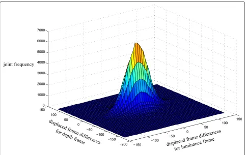
The authors of [22] propose the use of a Laplacian probability density function to model the displaced frame differences. In the case of noise-free video frames, the displaced frame difference image typically contains a small number of pixels with large values and a large number of pixels whose values are close to zero. However, in the presence of noise in the depth and luminance frames, displaced frame differences for both luminance and depth are dominated by noise. Large areas in the displaced frame difference image with values close to zero now contain noisy pixels as shown in Figure 4. Since the noise in the depth sensor is highly spatially variable, it is important to allow a non-constant noise standard deviation. We start from the model for displaced pixel differences in the pre-sence of noise from [23] and extend it to a multivari-ate case (i.e. the motion is estimmultivari-ated using both luminance and depth).

If we denote thea posterioriprobability given multiva-lued images F(t) and F(t- dt) as P(v(t)|F(t),F(t- dt)), from Bayes’s theorem we have

P(v(t)|F(t),F(t−dt)) =P(F(t)|v(t),F(t−dt))P(v(t)|F(t−dt)) P(F(t)|F(t−dt)) , (8)

where F(t) and F(t - dt) are the frames containing depth and luminance values for each pixel and v(t) is the motion vector between the framesF(t) andF(t-dt). The conditional probability that models how well the imageF(t) can be described by the motion vector v(t) and the imageF(t- dt) is denoted by P(F(t)|v(t), F(t -dt)). The prior probability of the motion vector v(t) is denoted byP(v(t)|F(t- dt)). We replace the probability P(F(t)|F(t- dt)) by a constant since it is not a function of the motion vectorv(t) and therefore does not affect the maximization process overv.

(6)

P(F(t)|v(t),F(t−dt)) = exp(

2

c=1

1 2(ν2

c+σc2) P

p=1

[F(l,t)−F(l−v,t−dt)]2₎

= exp( 1 2(ν2

L+σL2) P

p=1

[FL(l,t)−FL(l−v,t−dt)]2

+ 1 2(ν2

D+σD2) P

p=1

[FD(l,t)−FD(l−v,t−dt)]2),

(9)

where ν_D2 and ν_L2 are the variances of depth and lumi-nance blocks and σ2

L and σD2 are noise variances in the depth and the luminance images, respectively,l is the vector containing spatial coordinates of the current block, vis the motion vector of the current block, and FLandFDdenote the luminance and the depth

compo-nents ofF. Variances of the displaced pixel differences contain two components: one due to the random noise and the other due to the motion compensation error. The variance due to the additive noise is derived from the locally estimated noise standard deviation in the depth image and from the global estimate of the noise standard deviation in the luminance image. The use of the variance as a reliability measures for motion estima-tion in noise-free sequences was studied in [22,24].

A motion vector field can be modelled as a Gibbs ran-dom field, similar to [25]. We adopt the following model here for the prior probability of motion vectorv:

P(v(t)|F(t−dt))≈exp(−U(v(t)|F(t−dt))), (10)

where U is an energy function. We impose a local smoothness constraint on the variation of motion vec-tors by using the energy function, which assigns a smal-ler probability to the motion vectors that differ significantly from vectors in their spatio-temporal neigh-bourhood. We assume that a true motion vector may be very different from some of its neighbouring motion vectors, but it must be similar to at least one of its neighbouring motion vectors. For each of the candidate motion vectors, we define the energy function as the minimal difference of the current motion vector and its neighbouring best motion vectors:

U(v|F(t−dt)) = 1 2σ2

v

||v−vi||2, i∈Nv, (11)

(7)

expression for the energy function in Equation 8, we obtain the expression for our reliability to motion esti-mation as

P(v|F(t),F(t−dt)) =1

Kexp(−U(v(t)|F(t−dt))

− 1

2(ν2

L+σL2) P

p=1

− 1

2(ν2

D+σD2) P

p=1

[FD(l,t)−FD(l−v,t−dt)]2). (12)

This means that the motion vectors should produce small compensation errors in both depth and luminance (data term) and they should not differ much from the neighbouring motion vectors (regularization term). If we denote the set of all possible motion vector candidates asV and assume that v∈VP(v|F(t),F(t−dt)) = 1, we

obtain

K=

v∈V

exp−U(v(t)|F(t−dt))

− 1

2(ν2

L+σL2) P

p=1

− 1

2(ν2

D+σD2) P

p=1

[FD(l,t)−FD(l−v,t−dt)]2 ⎞ ⎠.

(13)

Therefore, each of the motion hypotheses for the block in the central frame is assigned a reliability mea-sure, which depends on the compensation error and the similarity of the current motion hypothesis to the best motion vectors from its spatial neighbourhood. The rea-son we introduce these penalties is that the motion compensation error grows with the temporal distance and the amount of texture in the sequence. From the previous equations, it can be concluded that the current motion vector candidatevis not reliable if it is signifi-cantly different from all motion vectors in its neighbour-hood. Motion compensation errors of motion vectors in uniform areas are usually close to the motion compen-sation error of the best motion vector in the neighbour-hood. However, in the occluded areas, estimated motion vectors have values which are inconsistent with the best motion vectors in their neighbourhood. Therefore, the motion vectors in the occluded areas usually have lowa posterioriprobabilities and thus low reliabilities.

3.2 The proposed temporal filter

In this section, we describe a new approach for temporal filtering along the estimated motion trajectories. The strength of the temporal filtering depends on the relia-bility of estimated motion.

The proposed temporal filtering is performed on all noisy wavelet bands of depth ˆsD₍_k_,_t₎ _{as follows:}

ˆ

sD(k,T) =

T+w₂

t=T−w₂

h∈H

α(h,t)sD(h,t), (14)

where ˆsD₍_k_,_T₎ _{is the temporally filtered version of the} depth wavelet band at the location kof the frame that is in the middle of the temporal buffer. Furthermore,sD(h, t) is the depth wavelet coefficient from the frameF(t) at the locationh.

The amount of filtering is controlled through the weighting factors a(t,h), which depend on reliability of the motion estimation defined in Equation 12. Weight-ing factors derived from conditional probabilities are also used in [23] for motion-compensated de-interlacing and in [26] for distributed video coding purposes. In the ideal case, motion estimation would be performed per wavelet band and reliabilities derived accordingly. Here we use same motion vectors for all wavelet bands, and calculate the reliability for each wavelet band separately, which can be justified by the fact that motion is unique.

The weights in their final form are derived from Equa-tion 12 by substituting the pixel values with the values of the wavelet coefficients at the same location:

α(t,h) =P(v|s(t),s(h,t−dt)), (15)

wheres(t) denotes the block of wavelet coefficients in the framet,s(h, t- dt) denotes the motion hypothesish in the framet- dtand H denotes the set of the motion hypothesis for the current block.P(v|s(t), s(h, t- dt)) has the form given in Equation 12.

We estimate the noise level by assuming that the noise variance at the locationkis related to the inverse of the signal amplitude assk=cn/A.

An important novelty is that we introduce a variable number of temporal candidate blocks used for denoising the block in the frame Ftvariable. Using all the blocks

within the support region of the sizews,Vt, t=T-ws/

2,..., T+ ws/2 for weighted averaging may cause some disturbing artefacts, especially in the case of occlusions and scene changes. In these cases, it is not possible to find blocks similar enough to the currently denoised block, which may cause over-smoothing or motion blur of details in the image. To prevent this, we only take into account the blocks whose average differences with the currently denoised block are smaller than some pre-determined thresholdDmax.

(8)

difference is Dmax

l = 3.5σl+ 0.7νl. By introducing the local noise standard deviation into threshold Dmax, we are taking into account the fact that even if we find a perfect match of the current block within the previous frame F(t- 1), it will differ from the current block in the frameF(t), due to the noise.

The proposed temporal filtering is also applied on the low pass band of the wavelet decomposition of both sequences, but in a slightly different manner. In the case of the low pass wavelet band, we set the smoothing parameter to the local variance of noise at location l. The value of the smoothing parameter for the low pass wavelet band is less than for high pass wavelet bands, since the low pass band already contains much less noise due to the spatial low pass filtering. In this way, we address the appearance of low-frequency artefacts present in the regions of the sequence that contain less texture.

The amount of noise is significantly reduced after the proposed temporal filter. To suppress the remaining noise, we use our earlier method for the denoising of static depth images [20].

This method first performs wavelet transform on both depth and amplitude images. Then, we perform the cal-culation of anisotropic spatial indicators using sums of absolute values of wavelet coefficients from both ima-ging modalities (i.e. the depth and the luminance). For each location, we choose the orientation which yields the biggest value of the sum. Based on values of spatial indicators, wavelet coefficients and locally estimated noise variance, we perform wavelet shrinkage of depth wavelet coefficients. The shape of input-output charac-teristics of the estimator is shown in Figure 5. It can be seen that the shape of the input-output characteristics of the estimator adapts to current values of the wavelet coefficients of both imaging modalities and correspond-ing spatial indicators, by shrinkcorrespond-ing depth wavelet coeffi-cients less in the case of large values of the current luminance wavelet coefficient and its corresponding spatial indicator. In the opposite case of small values of luminance wavelet coefficients and corresponding spatial indicators, depth wavelet coefficients are shrunk more, since there is no evidence in either modality that there is an edge at the current location. Adaptation to the local noise variance is achieved by simultaneously changing thresholds for the depth and the luminance. Since the initial value of the noise variance in depth is significantly reduced after temporal filtering, we propose to use a modified initial estimate of the noise variance. The variance of the residual noise in the temporally filtered frame is calculated using the initial estimates of noise standard deviation prior to temporal denois-ing and weights used for temporal filterdenois-ing as:

σ2 r =

t=1..T

h=1..Hα(t,h)2σ(t,h)2. The spatial method adapts to the locally estimated noise variance. Using this spatial filtering, the PSNR of the method is improved by 0.4-0.5 dB.

3.3 Basic complexity estimates

In this subsection, we analyse the computational com-plexity of the proposed algorithm. Motion estimation algorithm is performed over 7 depth and luminance frames, in a 24 × 24 pixels search window, on 8 × 8 pixel blocks. The main difference compared to classical gray-scale motion estimation algorithms is that the pro-posed algorithm calculates similarity metrics in both depth and luminance images, which doubles the number of arithmetical operations. In total,

12Nblocks Nf/2

t=1 NtcN2sN2b arithmetical operations are needed during the motion estimation step, whereNc= 2

is the number of the best motion candidates Nf= 7 is

the number of frames, tis a time instant, Ns= 24 size

of the search window,Nbis the size of the motion

esti-mation block andNblocksis the number of blocks in the frame. Then, we perform the wavelet transform and motion compensated temporal filtering in the wavelet domain. This step requires NblocksN_b2Nt arithmetical operations in total to calculate filtering weights and

NblocksN2_bNt additions to perform filtering, whereNtis

a total number of candidates which participate in filtering.

Finally, spatial filtering step requires (4 + (2K+ 1)2)L additions, 6L subtractions, 3Ldivisions and 4L multipli-cations per image, lomultipli-cations, whereKis the window size andLis the number of image pixels.

Compared to the method of [27], the number of operations performed in a search step is approximately the same, since we calculate similarity measures using two imaging modalities and choose a set of best candi-date blocks, while in [27] search is performed twice, using only depth information, first time on noisy depth pixels and second time on hard-thresholded depth esti-mates. Similarly, the proposed motion compensated fil-tering does not add much overhead, since filfil-tering weights are calculated during the motion estimation step. In total, number of the operations performed by the proposed algorithm and the method from [27] is comparable.

(9)

4 Experimental results

For the evaluation of the proposed method, we use both real sequences acquired using the Swiss Ranger SR3100 camera [28] and “noise-free”depth sequences acquired using ZCam 3D camera [29] with artificially added noise that approximates the characteristics of the TOF sensor noise.

To simulate the noise in the Swiss Ranger sensor, we add noise proportional to the inverse value of the ampli-tude. Since the luminance image of the Swiss Ranger camera is different from the amplitude image, we obtain the amplitude image from the luminance image by dividing it by the square of the distance from the scene and multiplying it by a constant [20]. Once the ampli-tude image is obtained, we add noise to the depth image whose standard deviation for pixell is proportional to the inverse of the received amplitude for that location. The example of the frames with simulated noise from the TOF sensor is shown in Figures 6 and 7.

We evaluate the proposed algorithm on two sequences with artificially added noise, namely “Interview” and

“Orbit”, and three sequences acquired using a Swiss Ranger SR3100 TOF camera. In the proposed approach, we use two levels of the non-decimated wavelet decom-position and Daubechies db4 wavelet.

We compare our approach with the block-wise non-local temporal denoising approach for TOF images of [10] and one of the best performing video denoising methods today VBM3D [27] using objective video qual-ity measures (PSNR and MSE) and visual qualqual-ity com-parison. Quantitative comparisons of the reference methods are shown in Figures 8 and 9. Average PSNR for tested schemes are given in Table 1. The results in Figures 6 and 7 demonstrate that the proposed approach outperforms the other methods in terms of visual qual-ity. The main reason for this is that the proposed method adapts the strength of spatio-temporal filtering

to the local noise standard deviation, while the other methods assume a constant noise standard deviation in the whole image. The noise standard deviation, required as an input parameter for the method of [27], is esti-mated using the median of residuals noise estimator from [30], denoted as“Case1” in Figures 10 and 11. In this case, the estimated standard deviations of noise for

“Orbit” and“Interview” sequences are 10.01 and 10.47, respectively. We also investigate the case when the noise standard deviation input parameter is equal to the maxi-mum value of the noise variance in the depth frame, i.e. 20, denoted as “Case2” in Figures 10 and 11. In this case, noise is completely removed from frames, at the expense of preserved details. The visual evaluation of the proposed and reference methods is shown in Figures 6b. and 7b. We can observe that the method from [10] removes noise uniformly in all regions. However, it tends to leave block artefacts in the image, due to its block-wise operation in the pixel domain. Some other fine details, like the nose, the lips, the eyes and the hands of the policeman in Figure 7 are also lost after denoising. If we observe Figures 6c and 7c, which show the results of [27], one can see that the details in the image are well preserved. However, one notices that the noise there is not uniformly removed, because the method of [27] assumes video sequences with stationary noise. Another drawback is that a certain amount of block artefacts is present around the silhouettes of the policemen.

On the other hand, the proposed method preserves details more effectively (see the details of the face in

“Interview” sequence). Furthermore, the surface of the table is much better denoised and closer to the noise free frame than in the case of the reference methods. Similarly, the mask and the objects behind in “Orbit” are much better preserved, while the noise is uni-formly removed. The boundaries of the object are −50 0 50 −50 0 50 −50 0 50 luminance depth output (a) −50 0 50 −50 0 50 −50 0 50 depth luminance output (b)

(10)

also preserved rather well, and do not contain the blocking artefacts as in the case of block-wise non-local temporal denoising. In the other scenario, we set the value of the input noise variance for [10,27] to the maximum local value of the estimated noise var-iance. Noise is now thoroughly removed. However, the sharp transitions in the depth image are severely degraded.

Finally, we evaluate the proposed algorithm on sequences obtained using the Swiss Ranger TOF sen-sor. All sequences used for the evaluation of the denoising algorithm were acquired using the following settings: the integration time was set to 25 ms, and the modulation frequency to 30 MHz. The depth sequences were recorded in controlled indoor condi-tions in order to prevent any outliers in depth images

(a) (b)

(c) (d)

(e) (f)

(11)

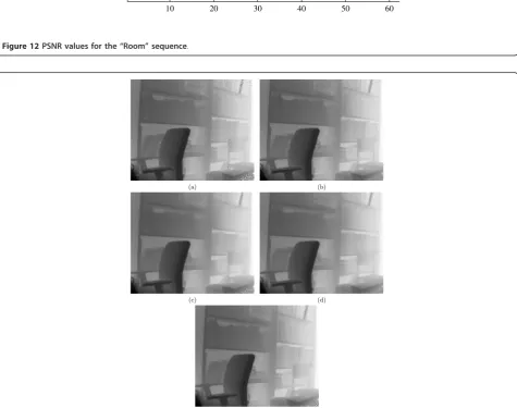
and the offset in the intensity image due to sunlight. All post processing algorithms of the camera were turned off. Noisy depth sequences which we use in the experiments are generated by choosing depth frames whose PSNR is median value of the PSNR values of each of the 200 frame sets. Values of PSNR for denoised sequences created using the Swiss Ranger TOF sensor are shown in Figures 10, 11 and 12, while

visual comparisons of results are shown in Figures 13 and 14.

We also compare 3D visualizations of the results pro-duced by different methods. Figure 15 shows the visuali-zations of the noisy point cloud, reference noise-free point cloud, point cloud denoised using the method of [27], and the point cloud denoised using the proposed spatially adaptive algorithm. The point cloud is

(a) (b)

(c) (d)

(e) (f)

(12)

represented by a regular triangle mesh, with the per face textures. As can be seen in Figure 15,z-coordinates of points from noisy point cloud differ significantly from the mean value represented by noise free image, which causes visual discomfort when displayed on 3D displays. The point cloud denoised using [27] contains much less variance than the noisy point cloud, especially in back-ground, but in the regions that have higher noise var-iance, like the hair of the woman, noise is still significant. It can be easily seen by observing Figure 15 that the point cloud denoised using our method removes almost all unwanted variations caused by noise from flat parts, while preserving fine details in range intact. Similar conclusions can be drawn after observing anaglyph 3D visualizations shown in Figure 16. Residual noise creates occlusions in both images and certain geo-metry distortion in the case where noise is not removed uniformly. On the other hand, the proposed method

removes noise uniformly without excessive blurring of edges, which creates visually plausible 3D images.

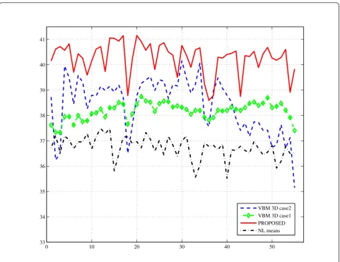
As in the previous cases, we compare the proposed method with the method of [27] for video sequences and with the method of [10] for denoising point clouds generated using structured light approach. The compari-son is performed using objective measures and visually. The PSNR values of the different methods are shown in Figure 10. A visual comparison of the proposed methods is shown in Figure 13. The methods used for compari-son [10,27] take a noise standard deviation as an input parameter. To provide these algorithms with the noise variance estimate, we used the median of residuals noise estimator from [30]. We can see from Figure 10 that the proposed method performs better than methods of [10,27] in all frames of the sequence. This is clearly visi-ble in Figure 13, especially at the borders of the images, where other methods fail to remove the noise of higher

0 10 20 30 40 50

33 34 35 36 37 38 39 40 41

VBM 3D case2 VBM 3D case1 PROPOSED NL means

(13)

intensity, while the proposed method removes noise in these regions quite successfully. Moreover, the edges of the books on the shelf, small surfaces like chairs and cir-cular object in the shelf are better preserved than when denoised with the reference methods.

5 Conclusions and future work

In this article, we have presented a method for removing spatially variable and signal dependent noise in depth images acquired using a depth camera based on the time-of-flight principle. The proposed method operates in the wavelet domain and uses multi hypothesis motion estimation to perform temporal filtering. One of the important novelties of the proposed method is that the motion estimation is performed on both depth and luminance sequences in order to improve the accuracy of the estimated motion. Another important novelty is that we use motion estimation reliabilities derived from both the depth and the luminance to derive coefficients for motion compensated filtering in wavelet domain. Finally, our temporal noise suppression is locally adap-tive, to account for the non-stationary character of the noise in depth sensors.

0 10 20 30 40 50 60 70

33 34 35 36 37 38 39 40 41 42

PROPOSED VBM case 2 NL means VBM case 1

Figure 9PSNR values for the_“Interview_”sequence.

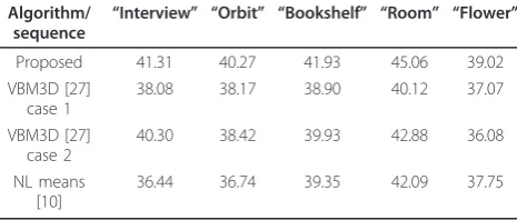
Table 1 Average PSNR values of the proposed and the reference algorithms in dB

Algorithm/ sequence “

Interview_{” “}Orbit_{” “}Bookshelf_{” “}Room_{” “}Flower_”

Proposed 41.31 40.27 41.93 45.06 39.02 VBM3D [27]

case 1

38.08 38.17 38.90 40.12 37.07

VBM3D [27] case 2

40.30 38.42 39.93 42.88 36.08

NL means [10]

(14)

0 5 10 15 20 25 30 35 40 45 30

32 34 36 38 40 42 44

Non−local Proposed VBM 3D case1 VBM 3D case2

Figure 10PSNR values for the“Bookshelf”sequence.

10 20 30 40 50 60 70

31 32 33 34 35 36 37 38 39 40

Proposed Non local VBM case2 VBM case1

(15)

10 20 30 40 50 60 34

36 38 40 42 44 46

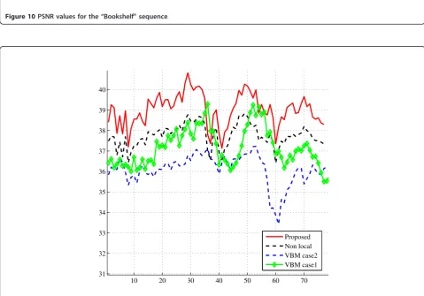
Proposed VBM case 1 VBM case 2 Non local

Figure 12PSNR values for the“Room”sequence.

(a) (b)

(c) (d)

(e)

Figure 138-th frame of the“Bookshelf”sequence: (a) noisy frame, (b) noise-free frame, (c) sequence denoised using method from

(16)

We have evaluated the proposed algorithm on several depth sequences. The results demonstrate improvement in this application over some of the best available depth and video sequences denoising algorithms ([10,27])

In future work, we will investigate GPU-based imple-mentation and motion estimation with a variable block size.

(a) (b)

(c) (d)

(e)

Figure 14 17-th frame of the“Flower”sequence: (a) noisy frame, (b) noise-free frame, (c) sequence denoised using method from[27], (d) sequence denoised using method from

[10], (e) sequence denoised using the proposed method.

(a) (b)

(c) (d)

Figure 153D rendering of the 5th frame of the_“Interview_”sequence: (a) noisy frame, (b) noise-free frame, (c) sequence denoised using method from[27], (d) sequence denoised using the proposed method.

(a) (b)

(c) (d)

Figure 16Anaglyph 3D visualization of the 5th frame of the

(17)

Acknowledgements

This study was funded by FWO through the Project 3G002105.

Competing interests

The authors declare that they have no competing interests.

Received: 5 June 2011 Accepted: 12 December 2011 Published: 12 December 2011

References

1. R Lange, P Seitz, Solid-state time-of-flight range camera. IEEE J Quant Electron.37(3):390–397 (2001). doi:10.1109/3.910448

2. A Kimachi, S Ando, Real-time phase-stamp range finder using correlation image sensor. IEEE Sensors J.9(12):1784–1792 (2009)

3. DV Nieuwenhove, W van der Tempel, R Grootjans, J Stiens, M Kuijk, Photonic demodulator with sensitivity control. IEEE Sensors J.7(3):317–318 (2007)

4. M Lindner, A Kolb, Lateral and depth calibration of pmd-distance sensors. ISVC.2006(2006)

5. T Kahlmann, F Remondino, H Ingensand, Calibration for increased accuracy of the range camera swissranger. ISPRS.2006(2006)

6. O Steiger, J Felder, S Weiss, Calibration of time-of-flight range imaging cameras. ICIP.2008(2008)

7. I Schiller, C Bedder, R Koch, Calibration of a pmd-camera using a planar calibration pattern with a multi-camera setup. ISPRS.2008(2008) 8. M Frank, M Plaue, FA Hamprecht, Denoising of continuous-wave

time-of-flight depth images using confidence measures. Opt Eng.48(7):077003– 1-077003-13 (2009). doi:10.1117/1.3159869

9. O Schall, A Belyaev, H-P Seidel, Error-guided adaptive fourier-based surface reconstruction. Comput Aided Design.39(5):421–426 (2007). doi:10.1016/j. cad.2007.02.005

10. O Schall, A Belyaev, H-P Seidel, Adaptive feature-preserving non-local denoising of static and time-varying range data. Comput Aided Design. 40(1):701–707 (2008)

11. T Schairer, B Huhle, P Jenke, W Stra_ber, Parallel non-local denoising of depth maps. International Workshop on Local and Non-Local Approximation in Image Processing (EUSIPCO Satellite Event). (2008) 12. J Kopf, MF Cohen, D Lischinski, M Uyttendaele, Joint bilateral upsampling.

ACM Trans Graph (TOG).26(3):96-1–96-6 (2007)

13. K-J Oh, S Yea, A Vetro, Y-S Ho, Depth reconstruction filter and down/up sampling for depth coding in 3-d video. IEEE Signal Process Lett. 16(9):747–750 (2009)

14. S Fleishman, I Drori, D Cohen-Or, Bilateral mesh denoising. ACM Trans Graph.22(3):950_–953 (2003). doi:10.1145/882262.882368

15. H Rapp, M Frank, F Hamprecht, B Jahne, A theoretical and experimental investigation of the systematic errors and statistical uncertainties of time-of-flight cameras. Int J Intell Syst Technol Appl.5(3/4) (2008)

16. R Lange, P Seitz, Solid-state time-of-flight range camera. IEEE J Quant Electron.37(3):390–397 (2001). doi:10.1109/3.910448

17. P Seitz, Quantum-noise limited distance resolution of optical range imaging techniques. IEEE Trans Circuits Syst I Regular Pap.55(8):2368–2377 (2008) 18. D Rusanovskyy, K Egiazarian, Video denoising algorithm in sliding 3d dct

domain. Lect Not Comput Sci.3708(3708):618_–626 (2005) 19. M Ozkan, A Erdem, M Sezan, M Tekalp, Efficient multiframe Wiener

restoration of blurred and noisy image sequences. IEEE Trans Image Process.1(4):453–476 (1992). doi:10.1109/83.199916

20. L Jovanov, A Pi_žurica, W Philips, Fuzzy logic-based approach to wavelet denoising of 3d images produced by time-of-flight cameras. Opt Exp 18(22):22651_–22676 (2010). [Online]. Available: http://www.opticsexpress. org/abstract.cfm?URI=oe-18-22-22651. doi:10.1364/OE.18.022651 21. X Jing, L-P Chau, An efficient three-step search algorithm for block motion

estimation. IEEE Trans Multimedia.6(3):435–438 (2004). doi:10.1109/ TMM.2004.827517

22. I Patras, E Hendriks, R Lagendijk, Probabilistic confidence measures for block matching motion estimation. IEEE Trans Circuits Syst Video Technol. 17(8):988_–995 (2007)

23. D Wang, A Vincent, P Blanchfield, Hybrid de-interlacing algorithm based on motion vector reliability. IEEE Trans Circuits Syst Video Technol.

15(8):1019–1025 (2005)

24. L Hill, T Vlachos, Fast motion estimation using a reliability weighted robust search. Electron Lett.37(7):418–420 (2001). doi:10.1049/el:20010311

25. J Konrad, E Dubois, Bayesian estimation of motion vector fields. IEEE Trans Pattern Anal Mach Intell14, 910–927 (1992). [Online]. Available: http:// portal.acm.org/citation.cfm?id=138791.138801. doi:10.1109/34.161350 26. N Deligiannis, A Munteanu, T Clerckx, J Cornelis, P Schelkens, Overlapped

block motion estimation and probabilistic compensation with application in distributed video coding. IEEE Signal Process Lett.16(9):743_–746 (2009) 27. K Dabov, A Foi, K Egiazarian, Video denoising by sparse 3d

transform-domain collaborative filtering. European Signal Processing Conference (EUSIPCO-2007). (2007)

28. Swissranger sr4000 overview, (2009) [online]. http://www.mesa-imaging.ch/ prodview4k.php

29. GJ Iddan, G Yahav, Three-dimensional Imaging in the Studio and Elsewhere. SPIE Three-Dimensional Image Capture and Applications IV.4298(1):48–55 (2001)

30. DL Donoho, Denoising by soft-thresholding. IEEE Trans Inf Theory.41, 613–627 (1995). doi:10.1109/18.382009

doi:10.1186/1687-6180-2011-131

Cite this article as:Jovanovet al.:Denoising algorithm for the 3D depth map sequences based on multihypothesis motion estimation.EURASIP Journal on Advances in Signal Processing20112011:131.