A comparison of approximation methods for the estimation of probability distributions on parameters

(1)

A Comparison of Approximation Methods for the Estimation of

Probability Distributions on Parameters

H.T. Banks and Jimena L. Davis

Center for Research in Scientific Computation

Box 8205

North Carolina State University

Raleigh, North Carolina 27695-8205

October 10, 2005

Abstract

(2)

1

Introduction and Theoretical Background

In this paper we consider approximation methods for a general class of estimation or inverse problems wherein the quantity of interest is a probability distribution. In particular we assume that we have a parameter (q∈Q) dependent system with model responsesx(q)describing in some manner a population of interest. For data or observations, we are given a set of values{zl}for the expected values

E[xl(q)|P] =

Z

Q

xl(q)dP(q)

with respect to an unknown probability distributionPdescribing the distribution of the parametersqover the population under investigation. We wish to use this data to choose from a given familyP(Q)the distributionP∗that gives a best fit of the underlying model to the data. Here we formulate an ordinary least squares (OLS) version of the problem, but this is not essential to our results and one could equally well use a weighted least squares, a maximum likelihood estimator, etc., approach. Thus we seek to minimize

J(P) =X

l

|E[xl(q)|P]−zl|2

overP∈ P(Q). Even for simple dynamics forxl, this is in general an infinite dimensional optimization

problem and approximations that lead to computationally tractable schemes are desirable. That is, it is useful to formulate methods to yield finite dimensional setsPM(Q)over which to minimizeJ(P). Of course, we wish to choose these methods so that“PM₍_Q₎_{→ P}₍_Q_)”_{in some sense. In this case we shall}

use the Prohorov metric [3, 15] of weak star convergence of measures to assure the desired approximation results. A general theoretical framework is given in [3] with specific results on the approximations we use here given in [2, 12]. Briefly, ideas for the underlying theory are as follows. One argues continuity ofP → J(P)onP(Q)with the Prohorov metric (this is trivial in the cases considered here). IfQis compact (again, easily established in our case) then it is known thatP(Q)is a complete metric space and is also compact when taken with the Prohorov metric. Moreover, if the approximation familiesPM₍_Q₎

are chosen so that elementsPM _{∈ P}M₍_Q₎_{can be found to approximate elements}_P _{∈ P}₍_Q₎_{in the}

Prohorov metric, then well-posedness (existence, continuous dependence of estimates on data, etc.) can be obtained.

The data{zl}available (which, in general, will involve longitudinal or time evolution data)

deter-mines the nature of the problem. The most classical problem (which we shall refer to as a Type I problem) is one in which individual longitudinal data is available for members in the population. In this case there is a wide statistical literature (in the context of hierarchical modeling, mixing distributions, mixed or ran-dom effects, mixture models, etc.) [14, 17, 18, 19, 20, 26, 27, 28, 29, 30, 33, 34] which provides theory and methodology for estimating not only individual parameters but also population level parameters and allows one to investigate both intra-individual and inter-individual variability in the population and data. In what we shall refer to as Type II problems one has only aggregate or population level longitudinal data available. This is common in marine, insect, etc., catch and release experiments [11] where one samples at different times from the same population but cannot be guaranteed of observing the same set of individuals at each sample time. This type of data is also typical in experiments where the organism or population member being studied is sacrificed in the process of making a single observation (e.g., certain physiologically based pharmacokinetic (PBPK) modeling [13, 21, 31] and whole organism trans-port models [11]). In this case one may still have dynamic (i.e., time course) models for individuals, but no individual data is available. Finally, the third class of problems which we shall refer to as Type III problems involves dynamics which depend explicitly on the probability distributionPitself. In this case one only has dynamics (aggregate dynamics) for the expected value

¯

x(t) =

Z

Q

x(t, q)dP(q)

(3)

approximations we discuss in this paper are applicable to all three types of problems, we shall illustrate the computational results in the context of size-structured marine populations where the inverse problems are of Type II.

Finally, we note that in the problems considered here, one can not sample directly from the probabil-ity distribution being estimated and this again is somewhat different from the usual case treated in some of the statistical literature, e.g., see [35, 36] and the references cited therein.

2

The Growth Rate Distribution Model and Inverse Problem

We now turn our attention to a specific application of the general ideas discussed above. The motivating application for this work is the estimation of growth rate distributions for size-structured mosquitofish populations. Mosquitofish have been used in the place of pesticides as a way to control mosquito pop-ulations in rice fields. Biologists desire to correctly predict the growth and decline of the mosquitofish population in order to determine the optimal densities of mosquitofish to use in rice fields to control mosquito populations. Thus, a mathematical model that accurately describes the mosquitofish popula-tion would be beneficial in this applicapopula-tion, as well as in other problems involving populapopula-tion dynamics and age/size-structured data.

Based on data collected from rice fields, a reasonable mathematical model would have to predict two key features that are exhibited in the data: dispersion and bifurcation (a unimodal density becomes a bimodal density) of the population density over time [4, 9, 10]. The growth rate distribution model, developed in [4] and [9], captures both of these features in its solutions. This model is a modification of the Sinko-Streifer model (used for modeling age/size-structured populations) which takes into account that individuals have different characteristics or behaviors. The standard Sinko-Streifer model (SS) for size-structured mosquitofish populations is given by

∂v ∂t +

∂

∂x(gv) = −µv, x0< x < x1, t >0 (1a)

v(0, x) = Φ(x) (1b)

g(t, x0)v(t, x0) =

Z x1

x0

K(t, ξ)v(t, ξ)∂ξ (1c)

g(t, x1) = 0. (1d)

In this model,v(t, x)represents the size (given in numbers per unit length) or population density, where t represents time andxrepresents the length of the mosquitofish. The growth rate of the individual mosquitofish is given byg(t, x),where

∂x

∂t =g(t, x)

for each individual, so that all mosquitofish of a given size have the same growth rate in this model. We also note thatµ(t, x)represents the mortality rate of the mosquitofish. The functionΦ(x)represents the initial size density of the population, whileKrepresents the fecundity kernel. The boundary condition atx=x0is the recruitment, or birth, rate, while the boundary condition atx=x1=xmaxensures the

maximum size of the mosquitofish isx1.The SS model cannot be used as is to model the mosquitofish

population because it does not predict dispersion or bifurcation of the population in time under biologi-cally reasonable assumptions [4, 9]. However, by modifying the SS model so that the individual growth rates of the mosquitofish vary across the population (instead of being the same for all individuals in the population), one obtains a model, known as the growth rate distribution (GRD) model, which does in fact exhibit both dispersal in time of the mosquitofish population and the development of a bimodal density from a unimodal density (see [9, 10]).

(4)

developed in [9], is actually given by

u(t, x;P) =

Z

G

v(t, x;g)dP(g). (2)

HereGis a collection of admissible growth rates,P is a probability measure onG,andv(t, x;g)is the solution of (1) with growth rateg.This model assumes that the population is actually made up of collections of subpopulations, where individuals in the same subpopulation have the same growth rate. Based on work in [9], solutions to this model exhibit both dispersion and bifurcation of the population density in time. For our considerations in this paper, we assume that the admissible growth rates have the form

g(x;b, γ) =b(γ−x)

forx0≤x≤γand zero otherwise, wherebis the intrinsic growth rate of the mosquitofish andγ=x1

is the maximum size. This choice is based on work in [4], where the idea of other properties related to the growth rates varying among the mosquitofish is discussed. Under the assumption of varying intrinsic growth rates and maximum sizes, we in fact assume thatbandγ are random variables taking values in the compact setsB andΓ, respectively. A reasonable assumption is that both are bounded closed intervals. Thus we take

G={g(·;b, γ)|b∈B, γ∈Γ}

so thatGis also compact in, for example,C[x0, X]whereX =max(Γ). ThenP(G)is compact in the

Prohorov metric and we are in the framework outlined above. In the first set of examples, we chose a growth rate parameterized by the intrinsic growth ratebwithγ= 1, leading to a one parameter family of varying growth ratesgamong the individuals in the population. We also assume here thatµ= 0and K = 0in order to focus on only the distribution of growth rates; however, distributions could just as well be placed onµandK.

We next introduce two different approaches that can be used in the inverse problem for the estimation of the distribution of growth rates of the mosquitofish. The first approach, which has been discussed and used in [9] and [10], involves the use of delta functions. We assume that the probability distributions PM _{placed on the growth rates are discrete corresponding to a collection}_GM _{with the form} _GM ₌

{gk}Mk=1 wheregk(x) =bk(1−x), fork = 1, . . . , M. Here the{bk}are a discretization ofB. For

each subpopulation with growth rategk,there is a corresponding probabilitypk that an individual is in

subpopulationk.The population densityu(t, x;P)in (2) is then approximated by

u(t, x;{pk}) =

X

k

v(t, x;gk)pk,

wherev(t, x;gk)is the subpopulation density from (1) with growth rategk.We denote this delta function

approximation method as DEL(M), where M is the number of elements used in this approximation. While it has been shown that DEL(M) provides a reasonable approximation to (2), a better approach might involve techniques that will provide a smoother approximation of (2) in the case of continuous probability distributions on the growth rates. Thus, as a second approach, we chose to use an approxima-tion scheme based on piecewise linear splines. Here we have assumed thatP is a continuous probability distribution on the growth rates. We approximateP0using piecewise linear splines, which leads to the following approximation foru(t, x;P)in (2):

u(t, x;{ak}) =

X

k

ak

Z

B

v(t, x;g)lk(b)db,

whereg(x;b) =b(1−x),pk(b) =aklk(b)is the probability density for an individual in subpopulation

kandlk represents the piecewise linear spline functions. This spline based approximation method is

(5)

probability distribution and N is the number of quadrature nodes used to approximate the integral in the formula above. We used the composite trapezoidal rule for the approximation of these integrals [32].

We were then able to use the approximation methods DEL(M) and SPL(M,N) in the inverse problem for the estimation of the growth rate distributions. The least squares inverse problem that we wish to solve is

min

P∈PM_(G)J(P) =

X

i,j

|u(ti, xj;P)−uˆ(ti, xj)|2 (3)

= X

i,j

(u(ti, xj;P))2−2u(ti, xj;P)ˆu(ti, xj) + (ˆu(ti, xj))2,

whereuˆ(t, x)is the data and PM(G)is the finite dimensional approximation to P(G). When using DEL(M), the finite dimensional approximationPM(G)to the probability measure spaceP(G)is given by

PM₍_G_{) =}

(

P ∈ P(G)|P0₌X

k

pkδgk,

X

k

pk= 1

) ,

whereδgkis the delta function with an atom atgk.However, when using SPL(M), the finite dimensional

approximationPM(G)is given by

PM(G) =

(

P ∈ P(G)|P0=X

k

aklk(b),

X

k

ak

Z

B

lk(b)db= 1

) .

Furthermore, we are able to note that this least squares inverse problem (3) becomes a quadratic programming problem [9, 10]. Letting p be the vector that containspk,1 ≤ k ≤ M, when using

DEL(M) orak,1≤k≤M,when using SPL(M,N), we let A be the matrix with entries given by

Akm=

X

i,j

v(ti, xj;gk)v(ti, xj;gm),

b the vector with entries given by

bk =−

X

i,j

ˆ

u(ti, xj)v(ti, xj;gk),

and

c=X

i,j

(ˆu(ti, xj))2,

where1≤k, m≤M.In the place of (3), we now minimize

F(p)≡pTAp+ 2pTb+c (4)

overPM₍_G₎_._{We note when using DEL(M) we also had to include the constraint}

X

k

pk = 1,

while when using SPL(M.N) we had to include the constraint

X

k

ak

Z

B

lk(b)db= 1.

(6)

3

Numerical Results

We next present and discuss several computational examples based on simulated data and performed in MATLAB involving the estimation of the probability distributionP on the growth rates of the size-structured mosquitofish population in order to demonstrate the validity of the theoretical results discussed earlier. The particular examples used here are based on previous formulations discussed in [4] and [9].

3.1

Convergence of DEL(M) and SPL(M,N) Estimated Probability Distributions

In order to estimate the probability distributionP∗_{on the growth rates of the size-structured mosquitofish}

population, we first began by preparing simulated population density data independent of the two approx-imation methods DEL(M) and SPL(M,N) used in the inverse problem. Since we were only concerned at this point with the estimation ofP∗_,_{we let} _µ _{= 0} _and_K _{= 0}_{in the Sinko-Streifer model. We}

then chose a true distributionP∗_{on the growth rates}_g₍_x₎_,_where_g₍_x_{) =}_b₍₁₋_x₎_and_b_{is the}

intrin-sic growth rate of the mosquitofish. More specifically, we assumed that the intrinintrin-sic growth rateb of the mosquitofish is a random variable with distributionP∗.This allowed us to generate a collection of growth ratesGn ={g1, g2, . . . , gn},where we tookn= 200in order to get a good approximation of

u(t, x;P∗_{) =}

Z

G

v(t, x;g)dP∗₍_g₎

andGn ⊂G.Our simulated dataud(t, x;P∗)was then created by first computing the solutionv(t, x;gi)

of the Sinko-Streifer model for each individualgiusing the method of characteristics and then computing

ud(t, x;P∗) =

Z

Gn

v(t, x;g)dP∗₍_g₎

using the Gauss-Legendre integration method( [32]). We took 50 uniformly spaced time observations, where the time interval was[0,0.5].The range of size values(x0, x1)was normalized to(0,1)and 50

uniformly spaced size values were used in this range for our simulated data. For the initial size density, we used

Φ(x) =

½

sin2₍₁₀_πx₎_, ₀_≤_x_≤₀_.₁_,

0, 0.1< x≤1.

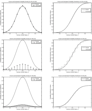
For our first set of data, we placed a “truncated” Gaussian distribution onbwith mean¯b = 4.5and varianceσ2 = 0.25, whereb ∈ [¯b−3σ,¯b+ 3σ].Using this range of values for the intrinsic growth rates allows us to capture approximately 99% of the intrinsic growth rates. However, to ensure that this “truncated” Gaussian distribution was indeed a true distribution, we had to scale the weights used in the Gauss-Legendre integration method to ensure that

Z ¯_b+3σ

¯b−3σ

f(b; ¯b, σ)db= 1, (5)

(7)

3 3.5 4 4.5 5 5.5 6 0

0.1 0.2 0.3 0.4 0.5 0.6 0.7 0.8 0.9

Known and Estimated Probability Density for SPL(15,200)

Intrinsic Growth Rates, b

Probability Density Coefficients

known estimated

3 3.5 4 4.5 5 5.5 6

0 0.1 0.2 0.3 0.4 0.5 0.6 0.7 0.8 0.9 1

Known and Estimated Probability Distribution for SPL(15,200)

Probability Distribution Values

known estimated

3 3.5 4 4.5 5 5.5 6

0 0.1 0.2 0.3 0.4 0.5 0.6 0.7 0.8

Known and Estimated Probability Density for DEL(15)

known estimated

3 3.5 4 4.5 5 5.5 6

0 0.1 0.2 0.3 0.4 0.5 0.6 0.7 0.8 0.9 1

Known and Estimated Probability Distribution for DEL(15)

known estimated

3 3.5 4 4.5 5 5.5 6

0 0.1 0.2 0.3 0.4 0.5 0.6 0.7 0.8

known estimated

3 3.5 4 4.5 5 5.5 6

0 0.2 0.4 0.6 0.8 1 1.2 1.4

known estimated

Figure 1:

Estimates of probability densities and distributions for true gaussian distribution using

a)SPL(15,200), b)DEL(15), c)DEL(45)

(8)

difference in the constraints for these two methods. SPL(M,N) requires X

k

ak

Z

B

lk(b)db= 1,

wherepk(b) =aklk(b)is the probability density for an individual in subpopulationkandlk(b)represents

the piecewise linear spline “functions.” On the other hand, DEL(M) requires X

k

pk = 1,

wherepk denotes the probability coefficients and δqk represents the delta functions. Since the true

density was in fact smooth and continuous, one would not expect convergence in density when using DEL(M) because it is much cruder in its approximation of (5). We remark that this agrees fully with the underlying theory for convergence of distributions in the Prohorov metric wherein convergence of densities is not guaranteed.

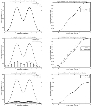
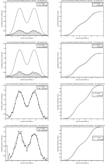
We also used a second set of data in the inverse problem with a “truncated” Bi-Gaussian distrib-ution on the intrinsic growth ratesb.Based on previous work in [4], this type of distribution leads to data which exhibits both dispersion and bifurcation, which are two traits observed in actual mosquitofish field data [4, 9, 10]. In order to obtain a Bi-Gaussian distribution, we took the average of two Gaussian distributions, one with mean¯b1= 3.3and varianceσ21= 0.492and the second with mean¯b2= 5.7and

varianceσ2

2= 0.492.The simulated data was prepared in the same way as described above except with

b∈[¯b1−3σ1,¯b2+ 3σ2].The results for the inverse problem using this set of data are shown in Figure

2 for SPL(25,200), DEL(25), and DEL(85). Both methods do a good job of estimating the Bi-Gaussian probability distribution with the simulated data. Again, we see that SPL(M,N) converges to the true dis-tribution faster than DEL(M). However, it should be noted that more basis elements (larger values of M) were required in both methods to achieve the same level of accuracy in approximating the Bi-Gaussian probability distribution in comparison to the Gaussian distribution. As mentioned earlier, the spline based approximation method results in both convergence in density and distribution for this example as well, while the delta function approximation method only results in convergence in distribution. We see that significantly more basis elements are required for full convergence of the approximations from DEL(M) to the true Bi-Gaussian probability distribution .

(9)

1 2 3 4 5 6 7 8 0

0.05 0.1 0.15 0.2 0.25 0.3 0.35

Known and Estimated Probability Density for SPL(25,200)

known estimated

1 2 3 4 5 6 7 8

0 0.1 0.2 0.3 0.4 0.5 0.6 0.7 0.8 0.9 1

Known and Estimated Probability Distribution for SPL(25,200)

known estimated

1 2 3 4 5 6 7 8

0 0.05 0.1 0.15 0.2 0.25 0.3 0.35

known estimated

1 2 3 4 5 6 7 8

0 0.1 0.2 0.3 0.4 0.5 0.6 0.7 0.8 0.9 1

known estimated

1 2 3 4 5 6 7 8

0 0.05 0.1 0.15 0.2 0.25 0.3 0.35

known estimated

1 2 3 4 5 6 7 8

0 0.2 0.4 0.6 0.8 1 1.2 1.4

known estimated

Figure 2: Estimates of probability densities and distributions for true bi-gaussian distribution using

a)SPL(25,200), b)DEL(25), c)DEL(85)

the quadrature rule gives a very coarse approximation to the actual integration, then we expectκ(A)

to become larger, the problem to become unstable, and the estimates of the probability distribution to become poor.

(10)

M

N

≈

κ(

A

)

5

50,100,150,200,250,300

9.35

25

50,100,150,200,250,300

87

55

50

10

17

55

100,150,200,250,300

10

4

75

50

10

19

75

100,150,200,250,300

10

5

95

50

10

18

95

100,150,200,250,300

10

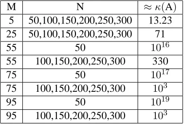
6

Table 1: Computed condition numbers of A for gaussian example when using SPL(M,N)

distribution when using SPL(5,N) and SPL(25,N). On the other hand, at M= 55,we began to see some significant differences inκ(A),as shown by the values in Table 1. It can be noted that for M= 55,75, and95, κ(A)was very large when using SPL(M,50). However, there was a significant decrease in the condition number of A when using SPL(M,N) for N= 100,150,200,250,300 for these values of M. This difference in condition numbers was also evident in the estimates of the probability distribution from the inverse problem. For M= 55,75,and95, the estimates when using SPL(M, 50) were worse than those obtained when using SPL(M,N) for all other listed values of N. We note the estimates of the Gaussian probability distribution became better as the value of N was increased for these fixed values of M.

M

N

≈

κ(

A

)

5

50,100,150,200,250,300

13.23

25

50,100,150,200,250,300

71

55

50

10

16

55

100,150,200,250,300

330

75

50

10

17

75

100,150,200,250,300

10

3

95

50

10

19

95

100,150,200,250,300

10

3

Table 2: Computed condition numbers of A for bi-gaussian example when using SPL(M,N)

For the Bi-Gaussian example, we also computedκ(A)for the same values of M and N, and the results in this case are given in Table 2. The results obtained when using a “true” Bi-Gaussian probability distri-bution were very similar to the results obtained when using a “true” Gaussian probability distridistri-bution. At M= 5and at M= 25, κ(A)was relatively small (13.23 and 71, respectively, for each value of N). The inverse problem for these values of M was also stable, and the estimates of the probability distribution in both cases were good. However, when M= 55,75,and95, SPL(M,50) results in large condition num-bers for A. The estimates for the probability distribution using SPL(M,50) were very poor in comparison to the estimates obtained from SPL(M,N) for M= 55,75,95and N= 100,150,200,250,300.When SPL(M,N) was used in the inverse problem for the estimation of the Bi-Gaussian probability distribution for M= 55,75,95and for values of N greater than 50, we saw a decrease in the condition numbers of A (see values in Table 2) corresponding to better approximations of the probability distribution.

(11)

when using SPL(M,N). However, when using SPL(M,N), for M ∼N,the condition number of A was very large, resulting in an ill-posed inverse problem and poor estimates of the probability distributions. For a fixed M, we observed that as the value of N increased, the condition number of A decreased, which agrees with results in [7] and [8]. Therefore, we have shown by these computational efforts that we can “regularize” the inverse problem when using SPL(M,N) by choosing proper ratios of M and N, which is known as “regularization by discretization balance.” By using a finer discretization in the quadrature method used in SPL(M,N), we were able to obtain better results in the inverse problem involving the estimation of growth rate distributions.

3.2

Sensitivity of DEL(M) and SPL(M,N) Estimated Probability Distributions

In the previous subsection, we discussed the results from two examples using simulated data in the estimation of probability distributions P on the growth rates of size-structured mosquitofish populations. However, data collected from an experiment is usually corrupted by noise, which can be a result of errors in collecting the data, errors in the instruments and techniques used, etc. Along with verifying that both SPL(M,N) and DEL(M) produce estimates which converge in distribution when simulated data with no noise is used in the inverse problem, we also wanted to be able to make some remarks about the sensitivity with respect to noisy data of the estimates of the probability distributions from the two approximation methods. Thus, we added random absolute noise to the simulated data used in the previous two examples in the following way:

ˆ

u(t, x;P∗) =u(t, x;P∗) +η·²,

whereη represents the noise level constant and²represents normally distributed random values with mean 0 and variance 1. We then performed the inverse problem again usingη = 0.005,0.025,0.05

corresponding to1%,5%and10%absolute error, respectively, for both the Gaussian and Bi-Gaussian cases.

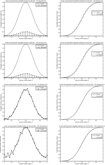
We begin by discussing the results of the inverse problem using the simulated data with a true “truncated” Gaussian distribution with the various noise level constants. Both approximation meth-ods, SPL(M,N) and DEL(M), performed decently in the inverse problem with the varying percentages of absolute error. With only 1%absolute error, both DEL(M) and SPL(M,N), with M and N chosen appropriately, resulted in estimates that converged to the true growth rate probability distribution in very much the same manner as discussed above in the Gaussian example with no noise. The performance of these approximations methods was not greatly effected by the small amount of noise in the data. With a slightly larger percentage of absolute error in the simulated data, SPL(M,N) and DEL(M) were still able to produce good estimates of the probability distribution. However, the results from the inverse prob-lem usingη = 0.025began to exhibit some small effects in the estimates obtained from both DEL(M) and SPL(M,N). For example, in Figure 3, the approximated probability distributions for DEL(25) and SPL(25,200) with5%absolute error reveal slightly overestimated front tails. Moreover, SPL(25,200) with5% absolute error resulted in small perturbations in the approximated density, which was very smooth when no noise was present in the data. With very noisy data,η= 0.05,SPL(M,N) and DEL(M) still perform fairly well. From the results for DEL(25) and SPL(25,200), shown in Figure 3, the noisier data resulted in only slightly poorer approximations in comparison to those obtained with5%absolute noise. Moreover, the larger amount of noise produced more oscillatory behavior in the approximated probability densities for both DEL(M) and SPL(M,N), which would result in poorer approximations of the corresponding probability distributions.

(12)

from DEL(M) and SPL(M,N) did not change significantly from the estimates obtained when there was no noise in the data. We were still able to obtain convergence in distribution (with faster convergence when using SPL(M,N)) with both approximation methods. When the percentage of absolute error in the data was5%,DEL(M) and SPL(M,N) still performed well by producing good estimates of the Bi-Gaussian probability distribution. The small amount of noise had some small effect on the estimates as seen in Figure 4; in fact, we see that the front tails in both the estimate from DEL(35) and SPL(35,200) for η= 0.025are slightly largely than the tails for the “true” distribution. When even more noise is present in the data, the estimated probability distributions became slightly poorer for a fixed M and N. In Fig-ure 4, the estimated probability densities and distributions are shown for DEL(35) and SPL(35) for data with10%absolute error. It is clear from these plots that the estimates from DEL(M) and SPL(M,N) are indeed affected by the noisier data. As in the Gaussian case, we noticed some oscillatory behavior in the estimated probability densities from these two approximation methods as the amount of noise present in the data increased. Moreover, the front tails in the estimated probability distributions are overestimated, whereas the end tails are underestimated for both DEL(35) and SPL(35,200).

(13)

3 3.5 4 4.5 5 5.5 6 0 0.1 0.2 0.3 0.4 0.5 0.6 0.7 0.8

Known and Estimated Probability Density for DEL(25) − 5% Absolute Error

known estimated

3 3.5 4 4.5 5 5.5 6

0 0.1 0.2 0.3 0.4 0.5 0.6 0.7 0.8 0.9 1

Known and Estimated Probability Distribution for DEL(25) − 5% Absolute Error

known estimated

3 3.5 4 4.5 5 5.5 6

0 0.1 0.2 0.3 0.4 0.5 0.6 0.7 0.8

known estimated

3 3.5 4 4.5 5 5.5 6

0 0.1 0.2 0.3 0.4 0.5 0.6 0.7 0.8 0.9 1

known estimated

3 3.5 4 4.5 5 5.5 6

0 0.1 0.2 0.3 0.4 0.5 0.6 0.7 0.8 0.9

Known and Estimated Probability Density for SPL(25,200) − 5% Absolute Error

known estimated

3 3.5 4 4.5 5 5.5 6

0 0.1 0.2 0.3 0.4 0.5 0.6 0.7 0.8 0.9 1

Known and Estimated Probability Distribution for SPL(25,200) − 5% Absolute Error

known estimated

3 3.5 4 4.5 5 5.5 6

−0.1 0 0.1 0.2 0.3 0.4 0.5 0.6 0.7 0.8

known estimated

3 3.5 4 4.5 5 5.5 6

0 0.1 0.2 0.3 0.4 0.5 0.6 0.7 0.8 0.9 1

known estimated

Figure 3: Estimates of probability densities and distributions for true gaussian distribution using a)DEL(25)

with

5%

absolute error, b)DEL(25) with 10

%

absolute error, c)SPL(25,200) with 5

%

absolute error,

(14)

1 2 3 4 5 6 7 8 0 0.05 0.1 0.15 0.2 0.25 0.3 0.35

known estimated

1 2 3 4 5 6 7 8

0 0.2 0.4 0.6 0.8 1 1.2 1.4

known estimated

1 2 3 4 5 6 7 8

0 0.05 0.1 0.15 0.2 0.25 0.3 0.35

known estimated

1 2 3 4 5 6 7 8

0 0.2 0.4 0.6 0.8 1 1.2 1.4

known estimated

1 2 3 4 5 6 7 8

0 0.05 0.1 0.15 0.2 0.25 0.3 0.35

known estimated

1 2 3 4 5 6 7 8

0 0.1 0.2 0.3 0.4 0.5 0.6 0.7 0.8 0.9 1

known estimated

1 2 3 4 5 6 7 8

0 0.05 0.1 0.15 0.2 0.25 0.3 0.35

known estimated

1 2 3 4 5 6 7 8

0 0.1 0.2 0.3 0.4 0.5 0.6 0.7 0.8 0.9 1

known estimated

Figure 4: Estimates of probability densities and distributions for true bi-gaussian distribution using

a)DEL(35) with

5%

%

absolute

(15)

3.3

Sensitivity Analysis of Approximation Methods with Respect to Noisy Data

We next considered the sensitivity of the two approximation methods, DEL(M) and SPL(M,N), with respect to noisy data in order to make some comments about the uncertainty associated with the estimated growth rate distributions. We cannot physically observe the entire population; however, we can include some measures (e.g., confidence intervals) on the uncertainty of the estimates obtained from the two approximation methods when using only a sample from the population. We follow the standard statistical framework for asymptotic (as sample sizen→ ∞) distributions for OLS estimators [19, 22, 25].

We began by considering the following statistical model for the mosquitofish population density

Y(¯xj) =f(¯xj, θ0) +²j, j= 1, . . . , n,

where{x¯j}corresponds to(tl, xm), l = 1, . . . , nt, m= 1, . . . , nxpairs (ntcorresponds to the number

of time values,nxcorresponds to the number of size values used, andn=nt·nx). We also note that

E[Yj] =f(¯xj, θ0) and var[Yj] =σ20,

whereθ0 ≈ θ = {pk}Mk=1 when using DEL(M) andθ0 ≈ θ = {ak}Mk=1 when using SPL(M,N) and

²j ∼ N(0, σ02).Here, θ0represents the “true” parameter value andσ02represents the “true” variance

for the system (which are generally not known) and theθ are the parameters to be estimated forθ0.

Furthermore, we note that

f(¯xj, θ0)≈ M

X

k=1

pkv(¯xj;gk), (6)

wheregk(x) =bk(γ−x),when considering DEL(M), while

f(¯xj, θ0)≈ M

X

k=1

ak

Z

B

v(¯xj;g)lk(b)db (7)

when considering SPL(M,N).

As stated previously, our goal is to quantify the uncertainty associated with the estimated growth rate distributions from the methods DEL(M) and SPL(M,N). We will make statements about the reliability of our estimates based upon standard errors. That is, we will compute confidence intervals corresponding to the estimated growth rate distributions. We note asn→ ∞,

ˆ

θOLS(Y)∼ NM(θ0, σ02[XT(θ0)X(θ0)]−1) =NM(θ0,Σ0),

whereX(θ) = ∂F

∂θ(θ) =Fθ(θ)is then×M sensitivity matrix with elements

Xjk(θ) =∂f(¯xj, θ)

∂θk .

We used the ordinary least squares estimator:

minimize inθ

n

X

j=1

(Yj−f(¯xj, θ))2.

The estimatesθˆfor the growth rate distribution minimize

n

X

j=1

(16)

for a particular realization or data set{yj}, and result from a quadratic programming problem as

dis-cussed earlier. As we have remarked, that along withθ0being unknown,σ0is also usually unknown.

Thus, in order to compute the standard errors associated withθ,ˆ we must also estimateσ0.We use the

following estimate forσ0:

σ2

0≈σˆ2=

1

n−M

n

X

j=1

³

yj−f(¯xj,θˆ)

´2

.

We then use these estimates to compute an estimate of the covariance matrixΣ0:

Σ0≈Σ = ˆσ2

h

XT(ˆθ)X(ˆθ)

i−1

.

Moreover, we note that the standard errors for the growth rate distributions estimatesθˆkare given by

SE(ˆθk) =

p

Σkk.

Before we present some results, we want to make a few comments about the covariance matrixΣ. We note that determiningσˆ2_{is very straightforward once we have}_θ._ˆ _{We simply multiply the residual at}

ˆ

θby _n₋1_M in order to computeˆσ2_._{We must also compute}_X_(ˆ_θ₎_,_{which can be more difficult in general}

when dealing with nonlinear systems. However, as we noted earlier, the elements of then×M matrix X(θ)are given by

Xjk(θ) =∂f(¯xj, θ)

∂θk .

These are actually the sensitivity elements associated with this system. We note for DEL(M) the entries in the sensitivity matrixX(θ)are given by

Xjk(θ) =∂f(¯xj, θ)

∂θk =v(¯xj, gk),

whereθk(pk or ak)is the probability parameter associated with growth rategk(x) = bk(γ−x).For

SPL(M,N), the entries in the sensitivity matrixX(θ)are given by Xjk(θ) =

∂f(¯xj, θ)

∂θk

=

Z

B

v(¯xj, g)lk(b)db.

Since both (6) and (7) are linear inθ,then computingX in this case is also very straightforward. Fur-thermore, the asymptotic distributional results given earlier are exact in this case (see [19, 22, 25]) as opposed to only being an approximation whenf(¯xj, θ)is nonlinear inθ.

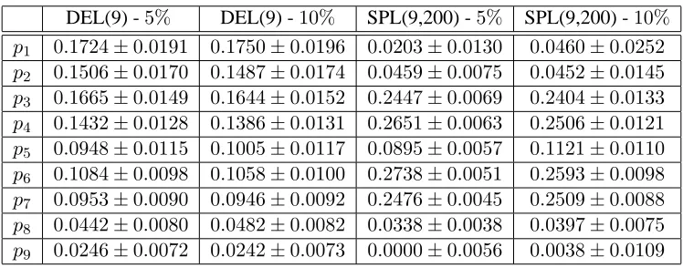
We present next some findings on the sensitivity of DEL(M) and SPL(M,N) using simulated data generated with a “true” Bi-Gaussian distribution. Table 3 displays the estimated probability density values and corresponding confidence intervals for DEL(9) and SPL(9,200) in the presence of5%and

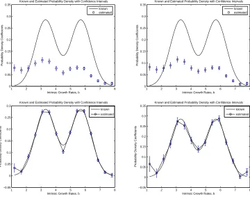
10%absolute error. In Figure 5, we see the confidence intervals corresponding to the estimated growth rate distributions withα= 0.05for DEL(9) and SPL(9,200) with simulated data with both5%and10% absolute error. The endpoints of the confidence intervals are given by

ˆ

θ±t1−α/2SE(ˆθ),

wheret1−α/2is a distribution value that is determined by the level of significance that is chosen [24].

After a level of significance is chosen, we determine the correspondingt1−α/2value from a statistical

table for the t-distribution. We chose to useα= 0.05for a significance level of95%,which corresponds tot1−α/2= 1.96when the number of degrees of freedom is large, i.e.,n≥30.Based on the confidence

(17)

DEL(9) -

5%

DEL(9) -

10%

SPL(9,200) -

5%

SPL(9,200) -

10%

p

1

0.1724

±

0.0191

0.1750

±

0.0196

0.0203

±

0.0130

0.0460

±

0.0252

p

2

0.1506

±

0.0170

0.1487

±

0.0174

0.0459

±

0.0075

0.0452

±

0.0145

p

3

0.1665

±

0.0149

0.1644

±

0.0152

0.2447

±

0.0069

0.2404

±

0.0133

p

4

0.1432

±

0.0128

0.1386

±

0.0131

0.2651

±

0.0063

0.2506

±

0.0121

p

5

0.0948

±

0.0115

0.1005

±

0.0117

0.0895

±

0.0057

0.1121

±

0.0110

p

6

0.1084

±

0.0098

0.1058

±

0.0100

0.2738

±

0.0051

0.2593

±

0.0098

p

7

0.0953

±

0.0090

0.0946

±

0.0092

0.2476

±

0.0045

0.2509

±

0.0088

p

8

0.0442

±

0.0080

0.0482

±

0.0082

0.0338

±

0.0038

0.0397

±

0.0075

p

₉

0.0246

±

0.0072

0.0242

±

0.0073

0.0000

±

0.0056

0.0038

±

0.0109

Table 3: Estimated probability density values and confidence intervals for true bi-gaussian distribution for

DEL(9) and SPL(9,200) with

5%

and

10%

absolute error

about the estimation procedure used to estimateθ0.In the results presented here, we can state that we are

95%confident that intervals constructed using the estimation procedures with DEL(M) and SPL(M,N) would “cover”θ0.We note that for the fixed valueM = 9the confidence intervals corresponding to

α = 0.05 when using DEL(M) are relatively small in relation to the estimatedθˆfor data with both

1 2 3 4 5 6 7 8

0 0.05 0.1 0.15 0.2 0.25 0.3 0.35

Known and Estimated Probability Density with Confidence Intervals

known estimated

1 2 3 4 5 6 7 8

0 0.05 0.1 0.15 0.2 0.25 0.3 0.35

known estimated

1 2 3 4 5 6 7 8

−0.05 0 0.05 0.1 0.15 0.2 0.25 0.3

known estimated

1 2 3 4 5 6 7 8

−0.05 0 0.05 0.1 0.15 0.2 0.25 0.3

known estimated

Figure 5: Estimates of probability densities with confidence intervals given a true bi-gaussian distribution

using a)DEL(9) with 5

%

absolute

(18)

5%and10%absolute error. Moreover, we note from Figure 5 that the resulting confidence intervals for DEL(9) with5%and10%absolute error are approximately the same. Thus, forM = 9, the delta function approximation method appears to be insensitive to noisy data. In comparison, we note for this fixed valueM = 9when using SPL(M,N) the resulting confidence intervals are relatively larger for data with10%absolute error in comparison to those for data with5%absolute error. Thus, the confidence associated with the estimator procedure based on SPL(M,N) appears to decrease as the percentage of absolute error increases. However, the confidence intervals are still relatively small in relation to the estimatesθ.ˆ Based on these results, we would infer that for this fixed value of M, the spline based approximation method appears to be very slightly sensitive to very noisy data.

1 2 3 4 5 6 7 8

0 0.05 0.1 0.15 0.2 0.25 0.3 0.35

known estimated

1 2 3 4 5 6 7 8

0 0.05 0.1 0.15 0.2 0.25 0.3 0.35

known estimated

1 2 3 4 5 6 7 8

−0.05 0 0.05 0.1 0.15 0.2 0.25 0.3

known estimated

1 2 3 4 5 6 7 8

−0.05 0 0.05 0.1 0.15 0.2 0.25 0.3 0.35

known estimated

Figure 6: Estimates of probability densities with confidence intervals given a true bi-gaussian distribution

using a)DEL(15) with 5

%

absolute error, d)SPL(15,200) with 10

%

absolute error

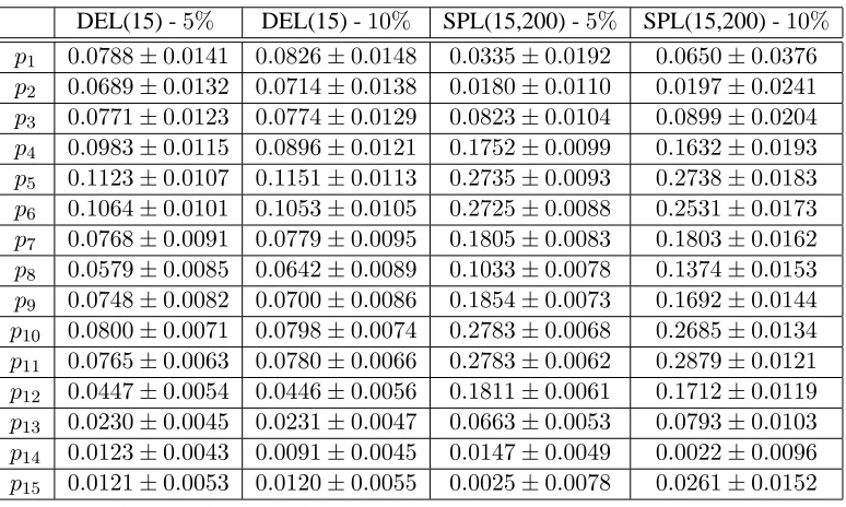
We note that the estimated probability density values and corresponding confidence intervals for DEL(15) and SPL(15,200) in the presence of 5%and 10% absolute error are given in Table 4. In Figure 6, we see the confidence intervals corresponding to the estimated growth rate distributions with α= 0.05for DEL(15) and SPL(15,200) with simulated data with both5%and10%absolute error. The endpoints of the confidence intervals are constructed in the same way as discussed above. We can again state that we are95%confident that intervals constructed using the estimation procedures with DEL(M) and SPL(M,N) would “cover”θ0.From Figure 6 we see that the confidence intervals corresponding to

α= 0.05when using DEL(M) forM = 15are relatively small in relation toθˆfor data with5%and

10%absolute error much like those computed forM = 9.We also see in this case that the confidence intervals are approximately the same for both sets of data. We arrive at the same conclusion forM = 15

(19)

DEL(15) -

5%

DEL(15) -

10%

SPL(15,200) -

5%

SPL(15,200) -

10%

p

1

0.0788

±

0.0141

0.0826

±

0.0148

0.0335

±

0.0192

0.0650

±

0.0376

p

2

0.0689

±

0.0132

0.0714

±

0.0138

0.0180

±

0.0110

0.0197

±

0.0241

p

3

0.0771

±

0.0123

0.0774

±

0.0129

0.0823

±

0.0104

0.0899

±

0.0204

p

4

0.0983

±

0.0115

0.0896

±

0.0121

0.1752

±

0.0099

0.1632

±

0.0193

p

5

0.1123

±

0.0107

0.1151

±

0.0113

0.2735

±

0.0093

0.2738

±

0.0183

p

6

0.1064

±

0.0101

0.1053

±

0.0105

0.2725

±

0.0088

0.2531

±

0.0173

p

7

0.0768

±

0.0091

0.0779

±

0.0095

0.1805

±

0.0083

0.1803

±

0.0162

p

8

0.0579

±

0.0085

0.0642

±

0.0089

0.1033

±

0.0078

0.1374

±

0.0153

p

₉

0.0748

±

0.0082

0.0700

±

0.0086

0.1854

±

0.0073

0.1692

±

0.0144

p

₁₀

0.0800

±

0.0071

0.0798

±

0.0074

0.2783

±

0.0068

0.2685

±

0.0134

p

₁₁

0.0765

±

0.0063

0.0780

±

0.0066

0.2783

±

0.0062

0.2879

±

0.0121

p

12

0.0447

±

0.0054

0.0446

±

0.0056

0.1811

±

0.0061

0.1712

±

0.0119

p

13

0.0230

±

0.0045

0.0231

±

0.0047

0.0663

±

0.0053

0.0793

±

0.0103

p

14

0.0123

±

0.0043

0.0091

±

0.0045

0.0147

±

0.0049

0.0022

±

0.0096

p

15

0.0121

±

0.0053

0.0120

±

0.0055

0.0025

±

0.0078

0.0261

±

0.0152

Table 4: Estimated probability density values and confidence intervals for true bi-gaussian distribution for

DEL(15) and SPL(15,200) with

5%

and

10%

absolute error

absolute error. We also see forM = 15as we saw forM = 9that the resulting confidence intervals are larger when the data is noisier. As discussed in the case forM = 9, the spline based approximation method also appears to be slightly sensitive to noisy data. To summarize, we note based on the standard error analysis discussed in this section and computational results (those presented here as well as those obtained forM = 5) we can conclude that DEL(M) appears to be insensitive to noisy data. Moreover, we can state that we are confident about the estimated growth rate distributions obtained using this method. We also conclude that SPL(M,N) appears to be relatively insensitive to noisy data. Furthermore, we would feel certain about the estimated growth rate distributions obtained using SPL(M,N) with data with small amounts of noise; however, we would infer that larger amounts of noise in the data would lead to larger confidence intervals and less certainty in the associated estimated growth rate distributions obtained using SPL(M,N).

4

Computational Results for Inverse Problems with Field Data

In this section, we will present and discuss the results of the inverse problem for the estimation of growth rate distributions using the delta function approximation method, the spline based approximation method, and a parameterized ordinary least squares method. We use field data collected from rice paddies in the place of the simulated data. Since the actual growth rate distribution of the mosquitofish observed in the experiment is unknown, we must compare the field data to the estimated population data produced by the estimated growth rate distribution from each of these methods in order to compare the efficacy of these methods.

In these numerical simulations, we assume that the growth rate of the mosquitofish is now para-meterized by both the intrinsic growth rateband the maximum sizeγ,whereg(x) = b(γ−x).The collection of growth rates for the DEL method is now given byG = {gjk},forj = 1, . . . , M1, and

k = 1, . . . , M2,wheregjk =bj(γk−x)with{bj}and{γk} the discretizations ofB andΓ,

(20)

thatµ= 0andK= 0,so that we can focus on the growth rate distribution only (mortality and fecundity were not thought to be important features of the experimental data of [4, 10]).

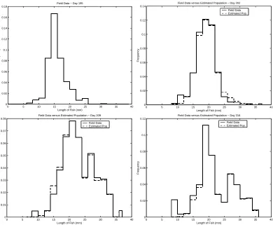
The field data that we are using in the inverse problem was collected in an experiment described in [10]. On June 28, 1992, four rice paddies were stocked with mosquitofish. In order to measure emigration, an outflow trap was placed on each paddy. Fifteen traps were used per paddy, and weekly measurements were taken. The length of the mosquitofish range from 0 to 40 mm, with the mosquitofish being grouped into size classes of 2 mm for a total of 20 size classes. The data for Day 195, Day 202, Day 209, and Day 216 are used in these simulations (see Figure 7). We define the size distribution frequency for size classiasfi=nm,i/Nm,wherenm,iis the number of mosquitofish measured in size

classiandNmis the total number of mosquitofish measured. The total population of mosquitofish is

divided into 512 subpopulations. We note that the discretizations for the intrinsic growth ratesband the maximum sizesγare defined as

bj = 0.2 + 1

31·4.8·(j−1), j= 1,2, . . . ,32

γ1 = 16

38, γ2=

22

38, γ3=

24 38

γk = 16

38+

1

15·

22

38·(k−1), k= 4, . . . ,16.

The Day 195 data is interpolated and used an approximation for the initial size densityΦ(x).Since this data set is used as an approximation forΦ(x), it cannot be used in the estimation of the growth rate distributions. Therefore, we are left with only three data sets to use in the inverse problem.

We introduced the delta function approximation method, DEL(M), earlier when the growth rate is parameterized bybonly. Since we are now considering a growth rate parameterized by bandγ,the approximated population density foru(t, x;P)in (2) is now given by

u(t, x;{pjk}) =

X

j,k

v(t, x;gjk)pjk,

wherev(t, x;gjk)is the subpopulation density from (1) with growth rategjkandpjkis the corresponding

probability that an individual has growth rategjk.We will now use the notation DEL(M1, M2) to denote

the delta function approximation method, whereM1 is the number of intrinsic ratesbj andM2is the

number of maximum sizesγkused in the approximation.

The spline based approximation method, SPL(M,N), was also introduced earlier for the one para-meter family of growth rates. For the two parapara-meter family of growth rates that we are now using, the approximated population density foru(t, x;P)in (2) is given by

u(t, x;{ajk}) =

X

j,k

ajk

Z

B

Z

Γ

v(t, x;g)lj(b)lk(γ)dγdb,

whereg=g(x;b, γ) =b(γ−x)andpjk(b, γ) =ajklj(b)lk(γ)is the probability density for individuals

in population subgroupjkwithlj,lk piecewise linear spline functions. The notation that we employ

here is SPL(M1, N1, M2, N2), whereM1andM2are the number of basis elements used to approximate

the growth rate probability distribution with respect tob andγ, andN1 andN2 represent the number

of quadrature nodes used in the composite trapezoidal rule [16] for double integrals to approximate the integral in the expression above with respect tobandγ.

We next present the results of the approximation methods DEL(M1, M2) and SPL(M1, N1, M2, N2),

(21)

the least squares inverse problem that we want to solve

min

P∈PM₁×M₂_(G)J(P) =

X

i,j

|u(ti, xj;P)−uˆ(ti, xj)|2

= X

i,j

(u(ti, xj;P))2−2u(ti, xj;P)ˆu(ti, xj) + (ˆu(ti, xj))2,

whereuˆ(t, x)is the data andPM1×M2(G)_{is the finite dimensional approximation to}P(G),_simplifies to a quadratic programming problem for an appropriately definedF(p)≡pTAp+ 2pTb+c.

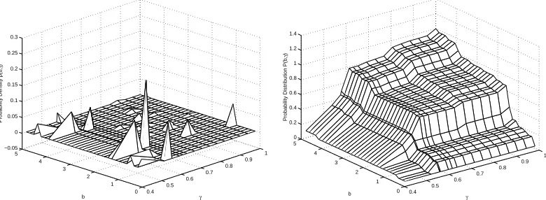
In Figure 7, we have the results from the inverse problem using DEL(32,16). These results were obtained in 514.3600 seconds, and the corresponding residualJ = 8.3169×10−4.We see from the results shown in Figure 7 that the estimated population is a good fit to the field data. The two key features of the data, dispersion and bifurcation, are both exhibited in the estimated population. The corresponding estimated probability density and distribution are shown in Figure 8. While no useful information can be obtained from Figure 8a, the estimated probability distribution in Figure 8b appears to be Bi-Gaussian in bothbandγ,which is expected based on results from [9] and [10].

0 5 10 15 20 25 30 35 40

0 0.02 0.04 0.06 0.08 0.1 0.12 0.14 0.16 0.18

Length of Fish (mm)

Frequency

Field Data − Day 195

0 5 10 15 20 25 30 35 40

0 0.02 0.04 0.06 0.08 0.1 0.12 0.14

Length of Fish (mm)

Frequency

Field Data versus Estimated Population − Day 202

Field Data Estimated Pop.

0 5 10 15 20 25 30 35 40

0 0.01 0.02 0.03 0.04 0.05 0.06 0.07 0.08

Length of Fish (mm)

Frequency

0 5 10 15 20 25 30 35 40

0 0.02 0.04 0.06 0.08 0.1 0.12

Length of Fish (mm)

Frequency

Figure 7: Field data versus estimated population for DEL(32,16)

The best results obtained using SPL(M1, N1, M2, N2) for the estimation of the growth rate

(22)

0.4 0.5 0.6 0.7 0.8 0.9 1 0 1 2 3 4 5 −0.05 0 0.05 0.1 0.15 0.2 0.25 0.3 γ b

Probability Density p(b,

γ ) 0.4 0.5 0.6 0.7 0.8 0.9 1 0 1 2 3 4 5 0 0.2 0.4 0.6 0.8 1 1.2 1.4 γ b

Probability Distribution P(b,

γ

)

Figure 8: a) Estimated probability density and b) estimated probability distribution for DEL(32,16)

SPL(5,35,5,35) and SPL(5,35,7,35). The corresponding residual,J, for SPL(5,35,9,35) is 0.0054, and these results were obtained in1.8822×103 _{seconds, or approximately 32 minutes. In comparison to}

the estimated population data produced by the estimated growth rate distribution from DEL(32,16), the estimated population data produced by the estimated growth rate distribution from SPL(5,35,9,35) does not give as good a fit to the field data, as is seen in Figure 9. The estimated probability density and distribution are shown in Figure 10. The resulting estimated probability distribution appears to be Bi-Gaussian inγ.In contrast to the results obtained in the previous examples with simulated data, the delta function approximation method does a better job of fitting the given field data in a more efficient way in comparison to the spline based approximation method.

Since the results from SPL(M1, N1, M2, N2) were not as good as those obtained from DEL(M1, M2),

we tried one more method in the inverse problem with the field data. Based on previous work in [9] and [10] and our own numerical simulations with simulated data, we know that a Bi-Gaussian growth rate distribution results in population density data with the two key features of dispersion and bifurcation. The field data that we are using in these computations exhibit these features as well, so we suspect that the un-derlying growth rate distribution is Bi-Gaussian. With that in mind, instead of approximating the density with delta functions or piecewise linear splines, we chose to use a parametric Bi-Gaussian probability density function in the growth rate distribution (GRD) model. The estimated{pjk} and{ajk}found

via the DEL(M1, M2) and SPL(M1, N1, M2, N2) methods, respectively, were not readily interpreted in

terms of the actual mosquitofish growth rate and maximum size means and variances. However, by us-ing an a priori Bi-Gaussian probability density function in the GRD model, we have in essence taken a standard parametric approach to the statistical inverse problem. The Bi-Gaussian probability density functionpwe choose is given by

p(b, γ; ¯b1, σb21,¯b2, σ

2 b2,γ¯1, σ

2 γ1,¯γ2, σ

2 γ2) =

    exp ½

−−(b−¯b1)2

2σ2

b1 ¾

2q2πσ2

b1

+

exp ½

−−(b−¯b2)2

2σ2

b2 ¾

2q2πσ2

b2     ×  exp n

−−(γ−¯γ1)2

2σ2

γ1 o

2q2πσ2

γ1

+

exp n

−−(γ−¯γ2)2

2σ2

γ2 o

2q2πσ2

γ2  

where we have assumed b and γ to be independent Bi-Gaussian random variables. The parameters

(¯b1,¯b2)and(σb21, σ

2

b2)represent the means and variances, respectively, of a Bi-Gaussian distribution on the intrinsic ratesb,while the parameters(¯γ1,¯γ2)and(σγ21, σ

2

(23)

0 5 10 15 20 25 30 35 40 0 0.02 0.04 0.06 0.08 0.1 0.12 0.14 0.16 0.18

Length of Fish (mm)

Frequency

Field Data − Day 195

0 5 10 15 20 25 30 35 40

0 0.02 0.04 0.06 0.08 0.1 0.12 0.14

Length of Fish (mm)

Frequency

0 5 10 15 20 25 30 35 40

0 0.01 0.02 0.03 0.04 0.05 0.06 0.07 0.08 0.09

Length of Fish (mm)

Frequency

Field Data versus Estimated Population − Day 209 Field Data Estimated Pop.

0 5 10 15 20 25 30 35 40

0 0.02 0.04 0.06 0.08 0.1 0.12

Length of Fish (mm)

Frequency

Field Data versus Estimated Population − Day 216 Field Data Estimated Pop.

Figure 9: Field data versus estimated population for SPL(5,35,9,35)

0.4 0.5 0.6 0.7 0.8 0.9 1 0 1 2 3 4 5 −0.5 0 0.5 1 γ b

Probability Density p(b,

γ ) 0.4 0.5 0.6 0.7 0.8 0.9 1 0 1 2 3 4 5 0 0.2 0.4 0.6 0.8 1 γ b

Probability Distribution P(b,

γ

)

Figure 10: a) Estimated probability density and b) estimated probability distribution for SPL(5,35,9,35)

Bi-Gaussian distribution on the maximum sizesγ.We will define q=¡¯b1, σ2b1,¯b2, σ

2 b2,γ¯1, σ

2 γ1,γ¯2, σ

2 γ2

¢ . Our third approach will not use an approximation to the GRD model, but instead use the Bi-Gaussian probability density function, given above, in the GRD model

u(t, x;q) = Z

B

Z

Γ

(24)

where againg(x;b, γ) =b(γ−x). We will denote this third approach as PAR(M, N1, N2), whereM is

the number of parameters in q andN1andN2represent the number of quadratures used in the composite

trapezoidal rule [16] to approximate the double integral with respect tobandγ,respectively. We will estimate q by solving the ordinary least squares problem

min

q∈RMJ(q) =

X

i,j

|u(ti, xj;q)−uˆ(ti, xj)|2,

whereuˆ(t, x)is the data. Once this least squares problem has been solved, we can use the optimal q in the Bi-Gaussian probability density function to determine the population densityu(t, x;q).

The optimal results for the inverse problem using PAR(8,35,35) are shown in Figure 11. The optimal parameters q= (1.9749,0.0388×10−3_,₃_.₉₁₃₂_,₀_.₂₂₂₈_×₁₀−3_,₀_.₅₂₆₅_,₀_.₇₂₀₈_,₀_.₀₁₂₂_,₀_.₀₃₇₂₎_,_with

a residualJ = 0.0074,were determined in 20.5490 seconds. In comparison to the results obtained using DEL(32,16) and SPL(5,35,9,35), the estimated population density does not fit the field data as well as the estimated population density produced by DEL(32,16) but is comparable to those obtained using SPL(5,35,9,35). We note that the spline based approximation method does a better job of estimating the frequencies for the smaller size classes than the parameterized OLS technique. While the results from the spline based approximation method and the parameterized OLS method are very similar, the computational time required by PAR(8,35,35) is much lower (compare the 32 minutes for SPL(5,35,9,35) versus 21 seconds for PAR(8,35,35)) than the computational time required by SPL(5,35,9,35). The estimated probability density and probability distribution generated by the optimal q are shown in Figure 12. We clearly see for a fixed value ofγthe probability distribution ofbis Bi-Gaussian.

As we did previously, we would like to also present here some results on the uncertainty associated with the estimated growth distributions determined by the inverse problem. The treatment in this section with the field data is very similar to the treatment previously carried out with the simulated data. With respect to the optimal results given in this section, we will only be able to perform a statistical analysis for SPL(5,35,9,35) and PAR(8,35,35). We are unable to perform this analysis for DEL(32,16) because the field data consists of 60 data points and the number of parameters determined by the DEL(32,16) is 512; thus, the analysis in this case is invalid. Since we have explained in detail the underlying statis-tical model that we are considering, we will omit these details here and define functions and variables that are used with respect to SPL(M1, N1, M2, N2) and PAR(M, N1, N2). First, we note that{x¯i}ni=1

corresponds to(tl, xm), l= 1, . . . ,3, m= 1, . . . ,20pairs since the field data that we use in the inverse

problem consists of three days and twenty size classes (hencen = 60),θ={ajk}M_j,k=11×M2 when using

SPL(M1, N1, M2, N2), andθ=q when using PAR(M, N1, N2). We also note that

f(¯xi, θ) = M1 X

j=1 M2 X

k=1

ajk

Z

B

Z

Γ

v(¯xi;g)lj(b)lk(γ)dγdb,