A comparison of robust estimators in simple linear regression

A COMPARISON OF ROBUST ESTIMATORS IN SIMPLE LINEAR REGRESSION

E. Jacquelin Dietz

North Carolina State University Raleigh, North Carolina

Key Words and Phrases: deficiency; intercept; point estimation; slope;' Theil estimator.

ABSTRACT

The mean squared errors of various estimators of slope, intercept, and mean response in the simple linear regression problem are compared in a simulation study. A weighted median estimator of slope proposed by Sievers (1978) and Scholz (1978) and two intercept estimators based upon it are

/

found to perform well for most error distributions studied. Theil's (1950) estimator of slope and two intercept estimators based on it are preferable for certain heavily contaminated error distributions.

1. INTRODUCTION

The topic of simple linear regression is either omitted entirely or covered incompletely in most popular nonparametric statistics texts. Many such books include a distribution-free test or confidence interval for the slope of the regression line, but omit any discussion of the intercept or the mean response at a given x.

paper, I investigate the mean squared erors of those same estimators in a simulation study.

2. THE ESTIMATORS

I assume the model Yi

=

C(

+

fJxi

+

ei , i

=

1,2, ... ,n, where C( and

fJ

are unknown parameters, xl ~ x2 ~ ... ~ xn are known constants (not all equal), and the ei's are independent and identically distributed continuous random variables with mean zero.

2.1 Slope Estimators

The estimators of

fJ

considered in this paper can all be viewed as functions of the N sample slopes

Sij

=

(Yj - Yi)/(Xj - Xi) , i L j , Xi

=

Xj .

If the Xi's are all distinct,

N

=

[~J

.

The following estimators of

fJ

are considered:

1. PLS

=

L

W' 'S'

'I L

W" where w' .

=

(x' - x,)2

, L ' 1J 1J ' L ' 1J ' 1J J . 1 .

A 1 J 1 J

2. flA

=

,L.Sij/N

(Randles and Wolfe,

1979,

Problem 3.1. 6).

A 1 LJ

3. flM

=

median of Sij'S (Theil,

1950).

A

Sij'S,

4.

_flWl

=

weighted median of _{where Wij}

=

j i.

A

S' .'s

5.

_fJw2

=

weighted median of _{1J '} where w· .1J

=

x'J

-

xi.

A

weighted median estimator (Sievers,

1978;

Scholz,

1978)

equals the median of the probability distribution obtained by assigning probability Wij/,~.wij to Sij.

1 J

2.2 Intercept Estimators

The estimators of C( considered in this paper can be divided into two groups, those that are functions of the N sample

intercepts

Aij

=

(XjYi - XiYj)/(Xj - Xi) , i L j, Xi

=

Xj ,

and those based on residuals associated with a particular slope estimate. The following estimators of C( are considered:

=

r

w}'J'A}'J'/

r

wiJ' , where w}'J'

=

(xJ' - Xi)2.

2. aA

=

L

Aij/N (Randles and Wolfe, 1979, Problem 3.1.6). iLj

3. aM

=

me~ian of Aij's.

A

4.

_a1,M

-

-

median of Yi flM xi

,

i

-

-

1,2,... ,n.

A

5. a1,W1

=

median of Yi flW1 xi i

=

1,2,... ,n.

A

6. a1,W2

=

median of Yi _{flW2 Xi} i

-

-

1,2, .•. ,n.

A

7. a2,M

=

median of pairwise averages of Yi - flM Xi·

A

8. a2,W1

=

median of painl1ise averages of Yi - flw1 xi·

A

9. a2,W2

=

median of pairwise averages of Yi

--

_{flw2 xi·}

A

10. ac

=

Y.50 -

flM

_x.50

,

_{where Y.50 and x.50 are the}

sam-pIe medians of the Y's and x's (Conover, 1980, p.267).

Bhattachar)~a (1968) considers estimators 7 and 8; Hettmansperger (1984) estimators 6 and 9.

2.3 Estimators of Mean Response

The mean response at a given x value, E(Y)

=

a +

fl

x, is often a more interesting parameter than the intercept a.

(Of course, if x ~ 0, then E(Y)

=

a.)

The estimators of E(Y) considered here are of the form a + P x, where eQch ~ is asso-ciated with the P with the same subscript, except that ~C is associated with

flM.

3. UNBIASEDNESS AND SYMMETRY

Certain unbiasedness and symmetry properties possessed by the estimators are important in the simulation study. Since

E(Sij)

=

p,

it follows that ilLS and ilA are unbiased estimators of

fl.

Sen (1968, Section 5) shows that the distribution of PM is symmetric about

fl,

and Theorem 5 of Sievers (1978) implies that PW1 and PW2 are asymptotically unbiased, under certain

conditions on the x's.

The assumption that the ei's have mean zero implies that E(Aij)

=

a and thus that cxLS and (xA are unbiased estimators of

symmetric error distributions, the two parameterizations coincide and all of the intercept estimators estimate the same parameter.

For symmetric error distributions all of the estimators of a

and {J in Section 2 except ~C have distributions that are

symmetric about the corresponding parameter. The distribution of

ac

is symmetric about a if {J

=

0; however, it does not seem possible to demonstrate any unbiasedness property for

ac

for general {J.

4. SIMULATION STUDY: METHODS

The bias and mean squared error (MSE) of the various estimators of slope, intercept, and mean response were estimated and compared in a simulation study. All computing was done in Fortran on the IBM 3081 at the Triangle Universities Computation Center. Medians of pairwise averages were computed using the algorithm of Monahan (1984), which in turn uses the uniform random number generator of Schrage (1979). The IMSL (1984) routines GGNML, GGUBS, and GGCHS were used to generate

no~mal, uniform, and chi square random numbers, respectively. The IMSL (1984) routine MSENO was used to calculate expected order statistics from the normal distribution.

Five hundred samples were generated for each combination of n

=

20 and 40, three x designs, and nine error distributions. Preliminary work indicated that this number of samples was sufficient to demonstrate highly significant differences among estimators.

All estimators of a and (3 considered here except ac have MSE's that do not depend on the values of a and {J. (The MSE of

ac

does not depend on the value of a, but does depend on (J.)

Thus, I set a

=

{J

=

O.

The value of each estimator of eX and (J defined in Section 2

was computed for each sample. For n

=

20 and the eight

distribution.) The five hundred values of an estimator thus obtained were used to estimate the bias and MSE of that estimator for that n, x design, and error distribution. The sample variances of the estimates and of the squared estimates over the 500 samples were used to estimate the variances of the bias and MSE estimates, respectively. An estimator will be

considered to show significant bias if the absolute value of its estimated bias exceeds two times the estimated standard error of the bias.

The first two x designs consisted of the expected order statistics from samples of size n from the uniform and normal distributions, respectively. The third x design, referred to as the double exponential design, was generated by calculating ±ar,

I' = 1,2, ... ,n/2, where

I'

ar

=

r

(n/2 - t

+

1) -1 ; t=l

a r is the expected value of the rth order statistic from a sample of size n/2 from the exponential distribution. Each set of x's was

n n 2

then standardized so that. 1. xi = 0 and. 1. xi = 1. For n = 20,

1=1. 1=1

E(Y) = 0:

+

(3 x was estimated for each of x = 20-. 5 = .2236 and x

= 2(20-. 5 ) = .4472, the x values one and two standard deviations from the center of the x's. These two x values and the values of x for each design for n = 20 are shown in Figure 1.

Nine error distributions were considered -- the standard normal, six contaminated normal distributions, the heavy-tailed t distribution with three degrees of freedom, and the asymmetric lognormal distribution. A single sample of n standard normal variates was used to generate samples from all nine error distributions. Specifically, for each of the 500 samples for a particular n value and x design, triples (Zi, Ui, Vi), i = 1,2,... ,n, were generated, where Zi is standard normal, Ui is Uniform (0,1), and Vi is chi-square with three degrees of freedom. Then the t3 and lognormal variates, standardized to have mean zero and

Contaminated normal (CN(k,o<)) samples, k

=

3,10 and 0<

=

.05, .10,

.25, were generated by multiplying each Zj by k with probability

0<, that is, if Ui fell in an appropriate interval:

k 0< Interval

3 .05 (.10,.15J

.10 (.15,.25J

.25 (.25 ,.50J

10 .05 (.50,.55]

.10 (.55,.65]

.25 (.65,.90]

As mentioned in Section 3, for asymmetric error

distributions the intercept parameter can be defined in different ways. The lognormal variates defined above have mean zero, but median (l - e 1/2 ) (e 2 - e)-1/2

=

-.3001675. For this error

distribution only, the bias and MSE of the intercept estimators were estimated in two ways -- with 0<

=

0 and 0<

=

-.3001675 as

the target parameter values. In addition, for the case of lognormal errors, normal x design, and n

=

20, I calculated the median of the 500 values of each intercept estimator, as well as the mean.

5. SIMULATION STUDY: RESULTS 5.1 Slope Estimators

The estimated MSE's of the slope estimators and the

associated standard error estimates are displayed in Table I for n=20. Results for n='l0 are similar and are not shown.

Simulation results for CN(k, .10) errors are intermediate to those for CN(k, .05) and CN(k, .25) errors, k = 3 and 10, and are

omitted from the table. Because of the unbiased ness results in Section 3, the estimated bias of the slope estimators is not

shown. As expected, the simulation results showed little evidence of significant bias in .the slope estimators. Note that for the uniform x design, PW1 and PW2 are identical.

TABLE I

Mean Squared Error of Slope Estimates, n=20

(Estimated Standard Errors in Parentheses)

x Design

Error

A

Distribution

{3

Uniform

Normal·

Double Exponential

N(O,l)

A

1. O( .06)

1.1( .06)

9.l( .57)

LS

1. O( .06)

1. O( .06)

1. O( .06)

M

1. O( .07)

1.1 ( .07)

1. 3( .08)

WI

1. O( .07)

1.1 ( .06)

1. 3( .08)

W2

1. O( .07)

1. 1( .06)

1.1( .07)

t3

A

.9( .08)

1. 2(

.11)

7.6( .60)

LS

.9( .07)

1.l( .10)

1. O( .12)

M

.6( .04)

.6( .04)

.8( .06)

WI

.6( .04)

.6( .04)

.8( .06)

W2

.6( .04)

.6( .04)

.7( .05)

CN(3, .05)

A

1. 6(

.11)

1.5( .10)

12.8( .93)

LS

1. 5( .10)

1. 4( .10)

1. 4( .12)

M

1. 2( .08)

1. 3( .08)

1.5( .10)

WI

1. 2( .08)

1. 2( .07)

1.5( .10)

W2

1. 2( .08)

1. 2( .08)

1. 3( .09)

CN(3, .25)

A

3.0( .20)

3.2( .20)

26. 8( 1. 95)

LS

2.8( .17)

2.9( .19)

2.8( .22)

M

1. 8( .12)

2.l( .14)

2.6( .18)

WI

1.a( .12)

2.l( .13)

2.5( .17)

W2

1.8( .12)

2.0( .14)

2.3( .19)

CN(lO, .05)

A

6.0( .61)

6.7( .59)

59.0(8.47)

I,S

5.8( .54)

5.8( .59)

6.5( .84)

M

1.2( .08)

1.4( .09)

1.6(

.11)

WI

1.

3( .09)

1. 3( .08)

1.

6(

.11)

W2

1. 3( .09)

1. 3( .08)

1.5( .10)

CN(lO, .25)

A

25.0(2.00)

27.9(1. 99)

235.4(20.81)

LS

23.7(1. 78)

25.1(1. 95)

24.3(1.78)

M

3.5( .30)

4.1( .39)

5.1( .51)

WI

3.9( .53)

4.4( .45)

.4( .57)

W2

3.9( .. 53)

4.9( .58)

5.9( .71)

Lognormal

A

1. O( .16)

1.1 (

.11)

10.4(1.40)

LS

1.0( .13)

.9( .09)

1.4( .52)

deficiency:

relative deficiency

=

1 - minimum variance variance

The minimum is taken over the estimators considered here. Deficiencies are all between zero and one, with one estimator assured a deficiency of zero. The graph of deficiencies for uniform x's is very similar to that for normal x's and is not shown. Note that since these estimators are unbiased, their variances are very similar to their MSE's, and thus the

estimators are ordered very similarly by MSE and deficiency. The unweighted average estimator 13A is clearly unacceptable in terms of MSE or deficiency, especially for the double

exponential x's and heavily contaminated error distributions. (In fairness to Randles and Wolfe (1979), they do not recommend this estimator or the intercept estimator Ct.A. These estimators arise merely as answers to a textbook exercise.) Not surprisingly, the least-squares estimator, 13LS, has the smallest MSE of any slope estimator for normally distributed errors. In almost every other case, however, the MSE of 13LS is exceeded only by that of 13A'

The estimator

13W2

performs well until the errors are heavily contaminated or asymmetric, at which point

13M

is preferable. The MSE of

13W1

is usually between those of

13M

and

13W2'

5.2 Estimators of Mean Response: Symmetric Errors

Estimation of ex is equivalent to estimation of E(Y)

=

ex

+

(3 x for x

=

0, and is discussed here in that context. The estimated MSE's of the estimators of mean response, along with their

estimated standard errors, are shown in Tables II and III for x

=

o

and x

=

.4472, respectively, and n

=

20. Results for x

=

.2236 are intermediate to those for the other x's and are not shown. Also, results for n

=

40 for x

=

0 are similar to those for n

=

20 and are not shown. The MSE's for CN(k, .10) errors are

intermediate to those for CN(k, .05) and CN(k, .25) errors, k

=

3 and

la,

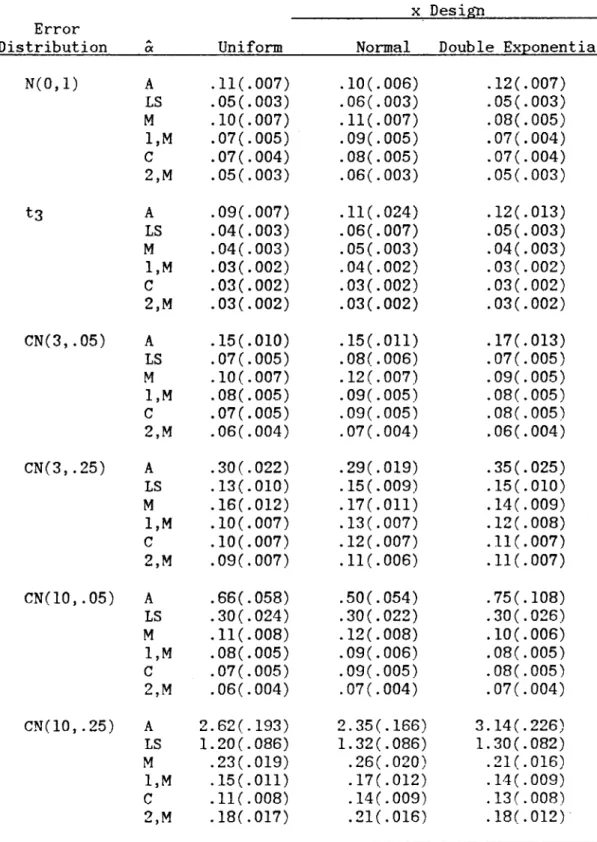
and are omitted from the tables. Results for the

TABLE II

Mean Squared Error of Intercept Estimates, n=20, Symmetric Error Distributions (Estimated Standard Errors in Parentheses)

x Design Error

Distribution A

Uniform Normal Double Exponential

ex

N(O,l) A .11(.007) .10(.006) .12(.007)

LS

.05(.003) .06(.003) · 05(.003) M .10(.007) .11 (.007) · 08(.005) I,M · 07(.005) · 09(.005) .07(.004) C · 07(.004) .08(.005) .07(.004) 2,M · 05(.003) .06(.003) .05(.003)

t3 A .09(.007) .11(.024) .12(.013)

LS

· 04(.003) .06(.007) · 05(.003) M · 04(.003) · 05(.003) · 04(.003) I,M · 03(.002) · 04(.002) .03(.002) C .03 (.002) .03(.002) .03(.002) 2,M .03(.002) .03(.002) .03(.002) CN(3, .05) A .15(.010) .15(.011) .17(.013)

LS

.07(.005) · 08( .006) .07(.005) M .10(.007) .12(.007) .09(.005) I,M .08(.005) .09(.005) · 08(.005) C .07(.005) · 09(.005) · 08(.005) 2,M .06(.004) .07(.004) · 06(.004) CN(3,.25) A .30(.022) · 29(.019) · 35(.025)

LS

.13(.010) .15 (.009) .15(.010) M .16(.012) .17(.011) .l4(.009) I,M .10(.007) .13 ( . 007) .12(.008) C .10(.007) .12(.007) .ll (.007) 2,M .09(.007) .11 (.006) .11 (.007) CN(lO, .05) A · 66(.058) .50(.054) · 75( .108)

LS

.30(.024) .30(.022) .30 ( .026) M .11( .008) .12( .008) .10(.006) I,M .08(.005) .09(.006) · 08(.005) C .07(.005) · 09(.005) · 08( .005) 2,M · 06(.004) .07(.004) .07(.004) CN(lO, .25) A 2.62(.193) 2.35(.166) 3.14(.226)

TABLE III

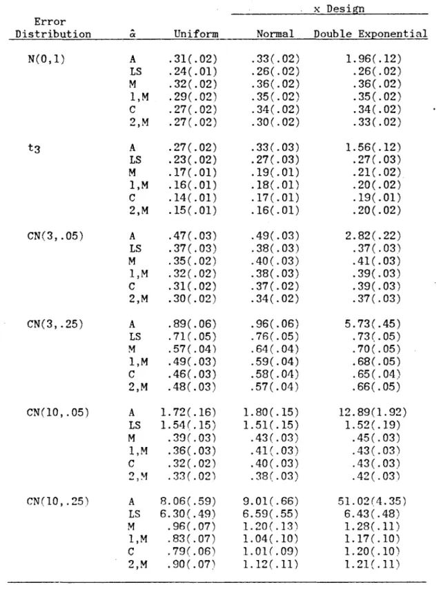
Mean Squared Error of Estimates of Mean Response n

=

20, x

=

.4472, Symmetric Error Distributions

(Estimated Standard Errors in Parentheses) x Design Error

Distribution A

Uniform Normal Double Exponential

ex

N(O,l) A .31(.02) .33(.02) 1. 96( .12)

LS

.24(.01) .26(.02) .26(.02)

M .32(.02) .36(.02) .36(.02)

I,M .29(.02) .35 ( . 02) .35( .02)

C .27(.02) .34(.02) .34(.02)

2,M .27 (.02) .30(.02) .33(.02)

t3 A .27(.02) .33(.03) 1. 56( .12)

LS

.23(.02) .27(.03) .27(.03)

M .17(.01) .19(.01) .21(.02)

I,M .16(.01) .18(.01) .20(.02)

C .14(.01) .17(.01) .19(.01)

2,M .15( .01) .16(.01) .20(.02) CN(3, .05) A .47(.03) .49(.03) 2.82(.22)

LS

· 37(.03) .38(.03) .37( .03) M · 35(.02) .40(.03) .41( .03) I,M · 32( . 02) .38(.03) .39(.03)

C .31(.02) .37(.02) .39(.03)

2,M .30(.02) .34(.02) .37( .03) CN(3, .25) A .89(.06) .96(.06) 5.73(.45)

LS

.71 (.05) .76(.05) .73(.05)

M .57(.04) . 64( . 04) .70 ( .05) I,M .49(.03) .59(.04) .68(.05) C .46(.03) .58(.0'1) .65( .04) 2,M .48( .03) .57(.04) .66(.05) CN(10, .05) A 1. 72( .16) 1. 80 ( .15) 12.89(1.92)

LS

1. 54( .15) 1.51( .15) 1.52(.19) M .39(.03) .43 ( . 03) .45(.03) I,M .36(.03) .41(.03) .43(.03)

C .32(.02) AO(.03) .43(.03)

2,M · 33( . 02) .38(.03) .42 ( .03) CN(lO, .25) A 8.06(.59) 9.01(.66) 51.02(4.35)

bias of the estimators is not shown. For n

=

20, no estimator of mean response showed significant bias for any symmetric error distribution.

As x increases from

a

to .4472, so that estimation of E(Y) increasingly involves extrapolation, the .MSE's of the estimators and their standard errors increase.

Certain conclusions hold for all combinations of x design, sample size, and x value included in the study. The unweighted

A A

average estimator OI.A

+

13

A x can be eliminated from consideration on the basis of its large MSE. The median estimator ;M + PM x is also noncompetitive; its MSE is usually one of the two or three largest. As expected, ;LS

+

PLSX is the best estimator for N(O,l) errors. However, for heavily contaminated normal errors and t3 errors, the MSE of ;LS

+

PLSX is usually exceeded only by that

A A

of OI.A

+

f3Ax.

For all combinations of sample size, x design, x value, and error distribution studied except the CN(10, .25) errors and the double exponential x design with x

=

.4472, the following results were found:

1. The estimators based on the ;l'S (;1,W1, 0I.1,W2, ;l,M) are very similar in MSE; the same is true of the estimators based on the ;2's (;2,Wb ~2,W2, ~2,M). In fact, for x

=

0, the MSE's of the three estimators within one of these groups rarely differ by more than .001; for x

=

.2236, by more than .01; and for x

=

.4472, by more than .02. Because of these similarities within the

~1

and

~2

groups, results for estimators based on

~1,W1'

0I.1"W2,

A A

0I.2,Wl, and 0I.2,W2 are omitted from Tables II and III.

2. The estimators based on the ;2'S have smaller MSE's than any other estimators for all symmetric error distributions studied except the N(O,l), for which they are second only to the least-squares estimator.

A

3. The MSE of the Conover estimator OI.C +

13M

x is usually between those of the ;1 estimators and the ;2 estimators.

following results were found:

1. The Conover estimator has the smallest MSE of all estimators considered.

A

2. Each <xl estimator has smaller MSE than the

corresponding ~2 estimator (that is, the ~2 estimator based on the same

11).

A

3. Within the <Xl and <X2 groups, the estimators based on

13M

have the smallest MSE's and those based on PW2 the largest. These patterns are shown graphically in Figure 4, which shows deficiencies of the estimators of mean response for uniform x's, n

=

20, x

=

0. Results for estimators based on ~l,Wl

=

<Xl,W2 and <X2,Wl

=

<X2,W2 are omitted from the figure. Deficiencies were calculated by taking the minimum variance over all intercept estimators, including those omitted from Figure 4.

For the double exponential x design with x

=

.4472

(excluding the CN(lO, .25) errors already discussed), the choice of

P

is more important than the choice between the ~l and ~2 groups. The estimators based on PW2 have the smallest MSE's; the MSE's ,of the estimators based on PWI and

PM

(including ~C +

PM

x but not ~M +

PM

x) are almost always within .02 of each other. Deficiencies of estimators based on

~1,W2' ~l,M' ~2,Wl'

and

~2,W2

are shown graphically in Figure 5. Deficiencies of estimators based on

~l,Wl, ~2,M' and ~C are between those of ~l,M and ~2,Wl for all symmetric error distributions. Note that x

=

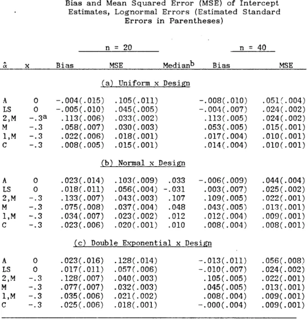
.4472 represents greater extrapolation for the double exponential x design than for the other x designs (See Figure 1.).

5.3 Intercept Estimators: Lognormal Errors

Simulation results for the lognormal error distribution are shown in Table IV and, for uniform x's, in Figure 4. As seen for

A

TABLE TV

Bias and Mean Squared Error (MSE) of Intercept Estimates, Lognormal Errors (Estimated Standard

Errors in Parentheses)

n

=

20 n

=

40

A

Bias MSE Medianb Bias MSE

C(

(a) Uniform x Design

A 0 -.004(.015) .105(.011) -.008(.010) · 05l(. 004)

L8 0 -.005(.010) .045(.005) -.004(.007) · 024(.002) 2,M -.3a .113( .006) .033(.002) .113(.005) · 024(.002)

M -.3 .058(.007) .030(.003) .053(.005) · 015(.001)

I,M -.3 · 022(.006) · 018(. 00l) .017(.004) .010(.001)

C -.3 .008(.005) .015(.001) . 014(.004) · 010(.001) (b) Normal x Design

A 0 .023(.014) .103(.009) .033 -.006(.009) .044(.004)

L8 0 · 018( .011) .056(.004) -.031 .003(.007) · 025(.002) 2,M -.3 .133(.007) .043(.003) .107 .109(.005) .022(.001) M -.3 · 075(.008) .037(.004) .048 . 043(.005) .013(.001) I,M -.3 · 034(.007) .023(.002) .012 .012(.004) .009(.001)

c

-.3 .023(.006) .020(.001) .010 .008(.004) · 008(. 00l) (c) Double Exponential x Design

A 0 · 023(.016) .128(.014) -.013(.011) · 056(.008)

L8 0 .017(.011) · 057(.006) -.010(.007) .024(.002)

2,M -.3 .128(.007) .040(.003) .105(.005) .022(.001)

M -.3 .077(.007) .032(.003) .045( .005) .013(.001)

I,M -.3 .035 ( . 006) .021(.002) .008(.004) .009(.001)

C -.3 .025( .006) · 018(. 00l) -.000(.004) .009(.001)

a Median of lognormal variates, actually -.3001675.

The bias and MSE of o:LS and O:A are computed using 0:

=

0 as the target parameter value. Neither estimator shows evidence of bias; ~LS is preferable to ~A in terms of MSE.

For all other estimators, the bias and MSE are computed using the median of the lognormal variates as the target parameter value.

A

This parameterization is appropriate for the three 0:1 estimators,

o:e,

and ~M' All show significant bias; however, for n

=

20 and the normal x design, the median of the 500 values of each of these

estimators (minus -.3001675) is closer to zero than is the mean of the 500 values, suggesting that these estimators are median unbiased. Of these estimators, ~M has the largest MSE.

The three ~2 estimators evidently estimate the pseudomedian of the lognormal distribution. The pseudomedian of a distribution F is the median of the distribution of (21

+

22)/2, where 21 and 22 are independent, each with distribution F (Hollander and Wolfe, 1973, p. 458). To estimate the pseudomedian of the lognormal distribution, I generated ten independent random samples of 10,000 lognormal variates each and found the median of pairwise averages for each sample. The median of these ten sample medians (minus -.3001675) was .10. This agrees moderately well with the estimated bias and median of ~2,M shown in Table IV.

It is interesting to note that cxLS, although unbiased, has larger MSE for estimating the mean than do the other estimators

(excluding ~A) for estimating the median. This is true despite the bias of the other estimators and the fact that ~2,M is not even estimating the "right" parameter.

6. SUMMARY

The main findings of the simulation study are:

1. The estimators

PA,

~A, and ~M can be eliminated from consideration because of their large MSE's.

2. The least-squares estimators, PLS and ~LS, have smaller MSE's than competitors for normal errors, but have very large MSE's for contaminated or asymmetric error distributions.

heavily contaminated or asymmetric, at which point

13M

is preferable.

4. For most situations considered, the estimators of mean response based on ;l's do not differ among themselves in MSE; neither do those based on cX2's. The cX~ estimators perform well until the errors are heavily contaminated or asymmetric, at which point the

a1

estimators and

aC

are preferable.

5. When estimation of the mean response requires

extrapolation, the choice of

13

estimator can be more important than the choice between the

a1

and

a2

groups of estimators. The estimators based on {JW2 perform well until the errors are heavily contaminated. Then the estimators based on PM are better.

BIBLIOGRAPHY

Andrews, D.F., Bickel, P.J., Hampel, F.R., Huber, P.J.,

Rogers, W.H., and Tukey, J.W. (1972). Robust Estimates of

Location. Princeton, New Jersey: Princeton University Press.

Bhattacharyya, G.K. (1968). Robust estimates of linear trend in multivariate time series. Ann. Inst •. Statist. hfath. 20, 299-310.

Conover, W.J. (1980). Practical Nonparametric Statistics (2nd edition). New York: Wiley.

Dietz, E.J. (1986). On estimating a slope and intercept in a nonparametric statistics course. Institute of Statistics Mimeograph Series No. 1689R, North Carolina State University.

Hettmansperger, T.P. (1984). Statistical Inference Based on Ranks. New York: Wiley.

Hollander, M. and Wolfe, D.A. (1973). Nonparametric Statistical hfethods. New York: Wiley.

International Mathematical and Statistical Libraries, Inc. (1984).

The IhfSL Library (9th edition). Houston, Texas: Author. Monahan, J.F. (1984). Algorithm 616. Fast computation of the

Randles, R.H. and Wolfe, D.A. (1979). Introduction to the Theory of Nonparametric Statistics. New York: Wiley. Scholz, F.W. (1978). Weighted median regression estimates.

Ann. Statist. 6, 603-609.

Schrage, L. (1979). A more portable Fortran random number generator. ACM Trans. Math. Software 5, 132-138.

Sen, P.K. (1968). Estimates of the regression coefficient based on Kendall's tau. Journ. Amer. Statist. Assoc. 63,

1379-1389.

Sievers, G.L. (1978). Weighted rank statistics for simple linear regression. Journ. Amer. Statist. Assoc. 73, 628-631. Theil, H. (1950). A rank-invariant method of linear and

Figure captions

FIG. 1 Positive values of x for n

=

20. The negative of each number is included also. x designs: 1 uniform; 2 normal; 3 -double exponential. Vertical dotted lines indicate x values for which E(Y) is estimated.

FIG. 2 Deficiency of slope estimators for normal x design, n

=

20. Error distributions: I-N{O,l); 2-t3; 3-CN{3,.05); 4-CN{3,.10);

5-CN{3,.25); 6-CN{l0,.05); 7-CN{l0,.10); 8-CN{l0,.25); 9 - lognormal.

FIG. 3 Deficiency of slope estimators for double exponential x design, n

=

20. Error distributions: I-N{O,l); 2-t3; 3-CN{3,.05); 4CN{3,.10); 5CN{3,.25); 6CN{10,.05); 7CN{10,.10); 8CN{10,.25); 9 -lognormal.

FIG. 4 Deficiency of intercept estimators for uniform x design, n

=

20. Error distributions: I-N{O,l); 2-t3; 3-CN{3,.05); 4-CN{3,.10); 5-CN{3,.25); 6-CN{10,.05); 7-CN{l0,.10); 8-CN{l0,.25); 9 - lognormal.

ZQH0m~

x

...

N

m

·

m

*

*

*

*

I

*

*

m

*

*

•

...

*

*

*

*

*

*

*

m

•

N

*

*

~---~---*

*

~

*

H

m

*

~

x

_•

w

~

*

*

*

m

• ~

-<OZfTlHOH"fTlO

(S) (S) IS) IS) (S)

-.

.

.

•

.

.

(S) I\) _~ 0)

<»

(S)

-

I

,

I

I

I

I

,

/

...

,

,

I ...

,

N

,

{

>

I

/

1

,

/

' /

,

' /

,

}

,

I

f

,

,

,

I

~,

fT1

I

:;0

I

:;0

.e..

I

0

1\

I

:;0

1 \

I

"":I

o·

I

H

H

I \

G")

I

.

_CfJ

w

-f

U1

I

L ...

_\

AJ

,

...

_\

H

m

I

...

\

C

I

...

\

-f

I

...

\

H

I

...

0

0>

...

,

\

...J-.

"

"

I ...

,"

,

"

l

/

..." " " - ,

,

I

/

" ..."""- "

,

(

\

/ 7 \

)

:

\

/

\

'

I

/ \\ '

I

\

\

'

' }

\

(

1,

I

\

I \

I

\

I

\

J

\

I

'

I

\

I

'

I

\

f

~

I

\

I

I

. \

""J

'--,

r--"

,

\

I

" "

'

\

' ' ' , , ' ,

\

"...'

)

,

\

~

I

I

"

\

\\

I

,

\

I

I

,

\

\

~

...

,...

I

I

\

\ "

\

'

I

\\

\

I

...

\

\

I

I

\

\

~

(

}

I

/

,

I

/

I / "

I

/

"

I

/

/ , / ' ,

/'

,

I

/'

/

/'

.'

0.25

N N

2,W2

1,W2

8

t

\

\

\

\

\

\

---""

\

\

/ '

"",

- - \

\

/ '

,

~

\

\

\

/

."

,

\

_\

\ . /

\

...,."

... "",

."

\

\

\

_,/

/

2,Wl

" \

\

' - - - - -

...

' , . "

,."

\

~

...

\ . /

~

I

I

\

' / \

I

"

\

\

----

--,

...

, . . .

...

...

\

""..1

1'-

"

\

... '"

... ...

\ I

""

I,M

\ . . .

\\ -'...

...

V

I

I

\...

.

6

7

I

5

I

e

88i

I

3 . .

.

·

I

2

ERROR DISTRIBUTION

.

9.29

D

E

F 0.15

I

C

I

E

~

0.10