Least square polynomial spline approximation

Thesis by

Paul David Patent

In Partial Fulfillment of the Requirements for the Degree of

Doctor of Philosophy

California Institute of Technology Pasadena, California

1972

ii

ACKNOWLEDGEMENT

I wish to thank Professor Robert P. Dilworth for his interest in my gener-al well being as a graduate student, Professor Martin H. Schultz for suggest-ing my thesis topic and many fruitful ideas concernsuggest-ing its investigation, and Professor Herbert B. Keller for his guidance in the preparation of the thesis itself.

I greatly appreciate the financial support which I have received from California Institute of Technology, the U. S. Office of Education through a National Defense Education Act Fellowship, and the Naval Undersea Research and Development Center through an Advanced Graduate Fellowship.

ABSTRACT

co

iv

CONTENTS

Acknowledgement . . . . ii

Abstract . • . . . . • . . . • . . . • . . iii

Introduction . . . 1

The Least Square Problem in Real Hilbert Space . . . . 3

'The Least Square Problem in L2{0, l] with Respect to Polynomial Spline Spaces . . . . 8

Quadrature Schemes of the Interpolatory Type . . . . 23

Quadrature Schemes of the Filan Type . . . . 39

Numerical Results . . . . 53

References . . . . 78

Appendix A - On an Inequality of E. Schmidt . . . . 80

Appendix B -A Cubic Spline Approximation Program - CSP LlT . . 85

Figures

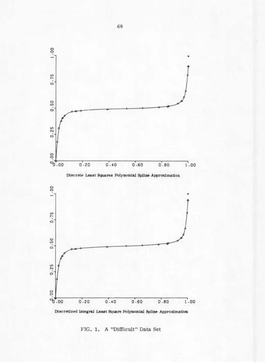
1. A "Difficult" Data Set . . . • . . . 68 2. Data for Ethanol- n-heptane Vapor Pressure • • • • • • • • • • • • • • . • 69 3. Data for Ocean Area Alpha - Winter • • . . • . • • . • • • • . • • • • . • • . 70 4. Data for Ocean Area Alpha - Spring. . • • • • . • • • . . • . • . . • • • . . . 71 5. Data for Ocean Area Alpha - Summer • • • • . • • • . • • • • • • . • • • • . 72 6. Data for Ocean Area Alpha - Autumn. • • • • • . . . • • • . • • • • • . • • • 73 7. Data for Ocean Area Bravo - Winter • • • • • • • . . • . • • . . . • • . • • • 7 4 8. Data for Ocean Area Bravo - Spring • • . • • • • • • • • • • . • . . • • • • • 75 9. Data for Ocean Area Gamma- Winter • • • • • • . • • • • • • • • • . • • • . 76

10. Program Listing for CSPLIT • • • • • • . • • • • • • • . • • • • . • . • . • • . 88 11. Program Listing for Subroutine CINPUT • • • • • • • • • . . • . . • . • . • 89

12. Program Listing for Subroutine PO LEX. • • • • • . • • . . . • • . . • • 90 13. Program Listing for Subroutine CDLS • • . • • • • • • . • • • • • . . • . • • 90 14. Program Listing for Subroutine CEVAL. • • • . • • . • • • • . • . . • . • • 91 15. Program Listing for Subroutine MATINV • . • • . • • • • . • • • • . . • • • 92

16. Progra_m Listing for Subroutine CMTRX . • . • • . . . • . • • • . . 93

vi

Tables

1. Least Square Linear Spline Approximation of the

Exponential Function . . . . • . • • . . . 56 2. Least Square Cubic Spline Approximation of the

Exponential Function . • . • . . . . • . . . • . . . 56

3. Least Square Cubic Hermite Spline Approximation of

the Exponential Function • . • • . . . • . . • . . . 57 4. Interpolatory Quadrature and Linear Spline Spaces . . . 59 5. lnterpolatory Quadrature and Cubic Spline Spaces . . . 60 6. lnterpolatory Quadrature and Cubic Hermite Spline

Spaces . • . . . . . . • . . . • • . . • . • . 61 7. Consistent Quadrature Schemes for Linear Spline Spaces . . . . . . 64 8. Consistent Quadrature Schemes for Cubic Spline Spaces • • . . . . • 65 9. Consistent Quadrature Schemes for Cubic Hermite

INTRODUCTION

In this paper we consider polynomial spline approximation t.echniques based on the theory of orthogonal projection in real Hilbert space. Splines are used as the approximations since they have smoothness properties and have been used to int.erpolat.e to large classes of smooth functions with small errors. In

addition, with the proper choice of basis functions, splines give rise to bounded well-conditioned matrices without orthonormalization. The motivation for the use of an integral least square technique is the hope that it might generate ap-proximations which would smooth errors due to "noisy" data. Int.erpolation t.echniques should be avoided, if possible, when attempting to approximate such data sets.

We begin, in Section 1, with a discussion of a least square approximation theory for finite dimensional subspaces of real Hilbert space. In Section 2,

we confine our att.ention to the Hilbe!'t space L2[0, 1] with inner product defined for g,hE:L2_{[0,1] by}

(g,h)

=

j

1

g(x) h(x) dx. 0

2

bound the L2-norms of the least square error and its derivatives. We then employ the L2-bounds to derive L00-bounds for the same error functions using a Sobolev type inequality. We discuss the application of techniques based on

1. THE LEAST SQUARE PROBLEM IN REAL HILBERT SPACE

In this section we formulate the least square problem in real Hilbert space.

We demonstrate the equivalence of this problem

to

that of solving an appropriate linear system of equations. The matrix involved is shown

to

be positive definite and symmetric thereby guaranteeing that a unique solution to the system of

equa-tions exists. We then conclude that a unique solution to the least square

prob-lem always exists. Finally, we discuss the context in which these concepts are

to be employed in this paper.

Let H be a real Hilbert space with the inner product of two elements f, gEH

denoted by (f, g). This inner product satisfies the following properties for all

f, g, hEH and any real number

a..

i) (a.f, g) ii) (f + g,h)

iii) (f' g)

a

(f, g) (f, h) + (g, h) (g, f)

iv) (f, f)

>

0 for f

f

0

v) (f, f) 0 for f == 0.

(1.1)

Then 11f11 - (f, f)l/2 _{defines a norm on Hand d(f, g) - 11 f - g 11 defines a metric}

4

Let G be any finite dimensional subspace of H. Then, given any f(H, we wish to find an element g(G which minimizes d(f,g)

=

llf - gll. We call this problem the least square problem for f ( H associated with the finite dimensional subspace G of H.

Suppose that the elements g_{1 ,} &;i, ••• , g₁₁ form a basis for G. Let Ct

=

(t:ici, ••• , a11 ) and define

F~ (1.2)

Clearly, our original problem is equivalent

to

finding an n-tuple

&

=

(&

_{1 , ••• ,} &₁₁) which minimizes F~. Using the definition of the norm

II· II

and the properties of the inner product ( · , · ) , we find that

F~

is a quadratic function of the

exp

1 s: i s: n. Consequently, the partial derivatives of F with respect to the a ₁, 1 s: i s: n, evaluated at such a minimum must equal

zero, i.e. , for 1 s: i s: n

oF

& oa@

1

n

-2(f, gt) + 2

L:

&J(gp gJ)

j=l

We shall write this system of equations, lmown as the normal equations, as

A

Aa. - k 0 (1.4)

where the entries, a₁J' of A and the components,

ki'

of£ are defined by

A

a₁J - (gpgJ), k_{1 -} (f,g_1), for 1 s i,j s n. (1.5)

Of course the matrix A is the well known Gram matrix or Gramian of the elements g_{1 , ••• ,} ~of H.

The matrix A is symmetric since (gpgJ)

=

(gJ,g₁₎ for alli,j by property (iii) of the inner product. Now given any n-tuple

q

= (a.1' ••• ,O!n)

(1.6)

6

Applying property (v) of the inner product yields

and, consequently, et ₁

=

0 all i, since the g_1, 1 ~ i ~ n, are linearly independent.

So et 1Acx :?: O with equality only if ex

=

O. Therefore, A is also positive definite. But then A has a unique inverse, A-1_{, and}

&

=

A-1~ _{is the unique solution to the} system (1.4). Therefore,

is the unique solution to the least square problem for f(H associated with the finite dimensional subspace G

=

span[g1 , ••• gn} of H. This completes the proof of the following well known theorem which is true, in fact, for any closed sub-space G of H and is known as the Projection Theorem.

Theorem 1.1-Given any f(H, the least square problem for f associated with G always has a unique solution.

Note that our proof of the theorem also provides a potential means by which such solutions may be obtained.

(g, h) -

£

1

g(x) h(x) dx

0

8

2. THE LEAST SQUARE PROBLEM IN L2[0, 1] WITH RESPECT TO

POLYNOMIAL SPLINE SPACES

In this section we first define the concept of polynomial spline spaces and state some standard spline interpolation results. We then examine, in detail, the least square problem in L2_{[0, 1] with respect}

to

_{these finite dimensional spaces}

of polynomial splines. We use L2_{-error bounds for polynomial spline}

interpola-00

tion

to

derive both L2_{- and L -error bounds for least square spline}

approxima-tion. We conclude with a discussion of the implementation of this technique.

We begin with the following definitions. For each non-negative integer, N, let 9t[O, 1] denote the set of all partitions,

A,

of the interval [O, 1] of the form

A:

o

1. (2.1)

00

Moreover, let&>[O, 1]

=

N

Yo

9PN[O, 1].

If

A

E&'N[O, 1], dis a positive integer and z is an integer such that -1 s; z s;d - 1, the polynomial spline space, Sp(d,

A,

z), is defined to be the set of all real valued functions s(x)E

cz[o,

1] such that, on each subinterval [xpx₁+₁

1,

O s; i s; N, of [0,1] determined by A, s(x) is a polynomial of degreed. Here, C-1_{[0,1] is} de-fined

to

be the set of all piecewise continuous functions on [O, 1] with each discon-tinuity a simple jump discondiscon-tinuity at one of the points xt' 1 ~ i ~ N. We note that Sp(d, A, z)

<;

L2[0, 1] and, since L2_{[0, 1] is a real Hilbert space with respect}

(g, h) -

£

1

g(x) h(x) dx, 0

we may study the least square problem for any ff:L2[0, 1] with respect t.o the finite dimensional subspace Sp(d,A,z). Theorem 1.1 applies and, consequently, we know that a unique solution t.o this problem always exists.

Note also that, for d = 2m - 1, m ~ 1, and m - 1 s: z s: 2m - 2 = d - 1, the definition of polynomial splines given here agrees with that of deficient splines of [l]. For generalizations of the concept of spline space, the reader is invited t.o study [16]. In fact, the polynomial spline interpolation results to be stated in this section remain essentially unchanged if one allows the integer z t.o depend on the partition points xit 1 s: i s: N, in such a way that

m - 1 s: z(x₁₎ s: 2m - 2.

As in [1], we define the interpolation mappingg.:c•-1[0,l]-Sp(2m - 1,A,z)

by .~f

=

s where

s; k s: 2m - 2 - z , 1 s: i s: N

(2.2)

, i=O,N+l.

The preceding interpolation mapping corresponds t.o the Type I interpolation

mapping of [ 16].

We shall soon need the following basic result on polynomial spline

10

Theorem 2.1-The interpolation mapping given by (2.2) is well defined for all AE.o/'[O, 1], 1 ::;; m, and m - 1 ::;; z ::;; 2m - 2.

Before we state the result which gives bounds for the error in polynomial spline interpolation, we must first make the following definitions. For each positive integer, p, let .KP [O, 1] denote the collection of all real valued functions, f(x), defined on [O, 1] such that f(CP-1_{[0, 1], DP-}1_{f is absolutely continuous, and} DPf(L2_{[0, 1] where Df}

=

_{df/dx denotes the derivative off. Also, given any}

following theorem is a composite of special cases of Theorems 3.5 and 4.1 of [14].

Theorem 2.2 - Let 1 ::;; m, 0 ::;; N, A(&'N[O, 1] and let m - 1 ::;; z ::;; 2m - 2. Then, for any f(l(2m[O, 1] and 0 ::;; j ::;; 2m,

(2.3)

[ (z - 2 + m) !]2

77an - J

[(z - 2 + m) !]2 j !7T:an - J

(z - 2 + m) !

77m if

if 0 $ j $ 2m - 2 - z,

if 2m - 2 - z < j $ m - 1,

m,

=

~

+ [ (z - 2 + m) ! + 2] [ (3m) !

JB

(A/

~J

- m , if m + 1 $ j $ 2m - 2,

1T 2m J 1T m

U

4m - j ) !

2 +[(z -2 +m)! +2]

r.

(3m)!

]\A!~m-1

if

=

_{2m -} l,

(2m - 1) !rr 77m u2m + 1) ! '

1 , if j

=

2m.

We note, as does the author of [14], that#.,f is not necessarily in Kl[O,l] for

z + 1 < j $ 2m and, in this case, we must define l!Dl(f -~f)llL

2

[0,l] by

These interpolation results enable us to give bounds for the L2_{-norms of the} error and its derivatives in approximating elements of certain classes of func-tions by polynomial splines using the least square technique of Section 1 of this

paper in the context described at the beginning of this section.

12

(g, h) -

f

1 g(x) h(x) dx. 0

As we have noted, L2[0, 1) is a Hilbert space with respect to this inner product since the norm which is induced by this inner product is the V3_-norm.

Conse-quently, the least square problem for any fEL2_{[0, 1] with respect to any finite}

dimensional subspace of L2_{[0, 1) always has a unique solution. In particular,}

if the subspace is a polynomial spline space, Sp(d,A,z), AE.o/'[0,1] and

-1 ~ z ~ d - 1, we shall denote the solutions. By definition,

s

is that element of Sp(d,A,z) which minimizes

lit-

s\\L₂[0,l] over Sp(d,A,z), i.e., for any sESp(d, A, z)

(2.5)

Now, if d

=

2m -1, fEI(2m[0,1] s;L2[0,1], and m -1 ~ z ~ 2m - 2, then.~f is a well-defined element of Sp(2m - 1, A, z) and, consequently,

Finally, Theorem 2.2 with j

=

0 applied to the right hand side of (2.6) gives us the following theorem in the case that j

=

0.

Theorem 2.3-Let 1 ~ m, 0 ~ N, AE-~[0,1] and m -1 ~ z ~ 2m - 2. For any function fE.K?n[0,1] s; L2_{[0,1], ifs is the least square approximation}

to

(2.7)

where

c

_m,z,J ~zo' ifj =O,

' '

K + 2 [ (2m - l) !

]'.:>

K (A//:;,,.\ J if 1 s J. s 2m - 1 ~"In, z, j (2m - j - 1) ! u.lll, z,o ~ '

=

l\i~z,2m' if j

=

2m, and (2.8)

the~ z J are given by (2.4).

'

'

Proof: We assume 1 s j ~ 2m - 1 since we have already established the result of the theorem in the case that j

=

0 and it is immediate in the case that j

=

2m since I)2m8

=

0 on [O, 1]. We shall need the following lemma which gives an in-equality of E. Schmidt that relates the L2_{-norm of the derivative of a polynomial} to the L2_{-norm of the polynomial itself. See Appendix A for a proof of this result.}

Lemma: Let Pm(x) be a polynomial of degree m on [a,b]. Then

11 11 (m + 1

>2

11 11

DPm L2_{[a,b] s b - a Pm L}2[a,b] · (2.9)

We now proceed with the proof of the theorem. We first use the triangle inequality to obtain

14

recalling that.~f is a well defined element of the spline space Sp(2m - 1,

A,

z)

to which

s

also belongs. Applying (2.9) j times to the second term on the right

hand side of the inequality (2.10) we obtain

j

1(

(2m - i)2

i=l

s: _ _ @_A_J_ l~f-

sllL2[0,l]

2

[ (2m - l) !

J

A -

J II

~f

'"'II

L<2m - j -1)! @ '• - s Vf0,1]

s: 2 [ (2m - 1) !

]21~\-

J

114'

9fll

L(2m - j - 1) ! ':=! !'" - •

Vto,

1] •

Combining (2.10) and (2.11) we obtain

(2.11)

(2.12)

s:

llDJ(f

'7_f)ll

+

2[

(2m -1)!

]2

A-J

II . II

-.m L2[0,1] L(2m-j-1)! @ f-~f L<l[0,1].

Finally, applying Theorem 2.2 to the terms on the right hand side of (2.12)

(2m - 1) ! - J - an an

[ ]

8

+ 2 (2m - j - 1) ! @

~,z,o(A)

II

D fllL2[0, 1)

(2m - 1) ! - J - 2 r J an

{

2 } (2.13)

~,z,J

+ 2f (2m - j - 1)

i]

(A/~

Km,z,o (A)

II

D fllL2[0, 1)

the result of the theorem in the case that 1 s: j s: 2m - 1.

We immediately have the following corollary.

Corollary: Given a sequence of partitions

[AJ}~

=

l

of [O, 1) such that

lim. AJ = O, if

s

J' for each j, is the least square spline approximation in J-a>

Sp(2m - 1,A,z), m - 1s:zs:2m - 2,

to

fe"I0'[0,1], then

~im

11

f -

s

J

II

L2[0, l] 0 · J-+00

If, in addition, (Al/AJ) s: Mall j, then, for 1 s:k s: 2m - 1,

00

We now introduce a lemma which enables us to derive bounds for the L -norm

of the least square error in terms of our bounds for the L 2-norm of this same

16

Lemma: Let u by absolutely continuous on [a, b] such that Du£ L2[ a, b]. Then

llullLCX)[a,b] s;

J2<P -

af112 llullL::i[a,b] +,/2(b - a)112 llDullL2[a,b].

(2.14)

Proof: For any x, x1 £[a, b]

and, consequently,

Squaring the inequality, we obtain

Therefore

and so

from which the result of the lemma follows immediately.

This brings us to the following theorem.

Theorem 2.4- Let 1 $ m, 0 $ N, AEBl'N[O, 1] and m - 1 $ z $ 2m - 2. For any

function frK21'1[0, 1]

S

L8[0, 1], ifs is the least square approximation to fin Sp(2m - 1, A, z), then, for 0 $ j $ 2m - 1,

(2.15)

where

(2.16)

sESp(2m - 1,

A,

z) is a polynomial of degree 2m - 1 on each subinterval [xpx₁+₁

1

of A, and consequently, nJsE:K1_{[xp xi+}

18

But (2.17) immediately implies that

(2.18)

We now apply the results of Theorem 2.3 to the terms on the right hand side of

(2.18) to yield

Again, the corollary is immediate.

Corollary: Given a sequence of partitions [ti.J}~

1

of [O, 1] such that

J-lim. AJ "' 0 and (Al/AJ) s; Mall j, if

sJ,

for each j, is the least square spline

J--+ CXl

-approximation in Sp(2m -1,A,z), m -1s;zs;2m - 2, to f{K2_{m[0,1], then, for}

O s; k s; 2m - 1,

~im

\I

D~f

- §J )\ \L oo[O, 1] 0.

J--+ CXl

Setting theoretical considerations aside, we now turn to the practical

prob-lem of actually obtaining such approximations. The proof of Theorem 1.1

im-mediately leads us to the question of basis functions for the finite dimensional

space of approximating functions. Let [

s

1

}~~

be a set of basis functions for the

NS-dimensional spline space, Sp(d, A, z). We note that NS

=

d + 1 + N(d - z).

In fact, the total number of indeterminates required to define an arbitrary

ele-ment of Sp(d, A, -1) is (N + 1) (d + 1) since we must determine the coefficients

of a polynomial of degreed on each of N + 1 subintervals of A and there are no

continuity constraints. In the case that there are constraints, and here we

con-sider the integer z to depend on the interior mesh points x1' 1 ~ i ~ N, continuity

of degree z (x₁₎ at Xp 1 s; i s; N, introduces z(x ₁) + 1 constraints and consequently

reduces the number of indeterminates by z(x₁) + 1. Therefore,

N

NS (N -+ l)(d + 1) - L(z(x₁) + 1)

i=l

d + 1 + Nd -

f

z(x₁)

20

which reduces to NS = d + 1 t N(d - z) in the case that z(x₁)

=

z, 1 s; is; N.

Now, for f(L2_{[0, 1], we have seen that the least square approximation to fin}

Sp(d,A,z) is

where

&

=

_{(Cxl' ••• , &N 5)} is the unique solution to the system

A

Aa. - k 0 (2.19)

A A

where the entries, a_{1 l,} of A and the components, k₁, of k are defined for

1 :s; i,j :s; NS by

atl

-

£

1

s1(x) sl(x) dx and

0

(2.20)

k1

-

f

1

f(x) s ₁(x) dx.

0

Therefore, in order to actually obtain the least square approximation to fin

Sp(d, A, z), i.e., calculate the NS-tuple

& ,

we must have numerical values for

the entries of A and the components of Ras well as an effective technique with

which to solve the system (2.19). Since A is positive definite and symmetric,

the point successive over-relaxation iterative method is guaranteed to converge

and can be used to determine

&

(cf. [17, p. 59]). Another possibility would be to

which indeed is the case when d = 2m - 1, m ~ 1, and m - 1 s; z s; 2m - 2 for

suitably chosen basis functions (cf. [13]), Gaussian elimination can be used to

efficiently solve the system (2.19). In any case, the zero structure of A

deter-mines the technique to be employed and its rate of convergence. In fact, once

the basis functions for Sp(d,

A,

z) are chosen, the entries of A may be calculated

directly as they are just sums of definite integrals of polynomials over

subin-tervals [x₁,x₁+1

1,

0 s; is; N, of

A.

Of course, the zero structure of A will then be

determined and the appropriate technique can be chosen. The possibility of

cal-culating the entries of

k

directly seems remote since we may not have a

represen-tation off which would admit such a calculation. Indeed, in many, if not most,

practical applications, f is a tabulated function, i.e., its value may be known at

only a finite number of discrete points. In such a situation, a quadrature scheme

of some sort must be used to obtain the NS-tuple ~. an approximation to ~. and

we solve the system

0 (2.21)

instead of (2.19). I.et

where

Ci

(ci

1 , • •• ,

ex

NS) is the unique solution to (2.21). Recalling that the

least square approximation is denoted

s,

we wish to bound 11

s -

s

11 in terms of

22

of consistency in the cases that bounds for

11

f - §

11

exist. To this end, let L

denote the integral over [O, 1] and let

L

be the quadrature rule used to determine

E'.,

both regarded as bounded linear functionals on C[O, 1]. Then

1 s; i s; NS, and

k

₁ =

Us

1' 1 s; is; NS, and beginning with (1.6), we find that

lls -

sllt21:a,b]

NS

L

(ex

1

-a

1)(L[fstl - L[fsd)

i=l

(L -

L)[f

f

(Ct

_{1 -} CX1)

s~

i=l

~

<L -

L)

[f<s -

s)J.

We shall use this relation in the next sections in order

to

develop our main

3. QUADRATURE SCHEMES OF THE INI'ERPOLATORY TYPE

In this section we first consider the concept of interpolatory quadrature and we derive error bounds for such schemes when applied to members of certain classes of functions. We then describe composite quadrature schemes (based on interpolatory formulae) which we shall use to obtain approximate solutions to the least square problems which we discussed in preceding sections. We study the error introduced into the approximation by the use of such a composite scheme. We examine the question of convergence for sequences of such approximations. We then define the concept of consistent quadrature schemes and conclude this section with an application of the discussion to the case at hand.

As in [8, p. 303], let the n + 1 distinct points T ₀ < T₁ < · ·-< T n be given so that a s: T J s: b for all j. Then, for any function CYEC[a, b], we may construct the interpolation polynomial, Pn(x), of degree at most n such that CY(TJ)

=

Pn(TJ) for all j. We take

as an approximation to

L*CT

lb

C1(X) dx.

a

(3 .1)

24

By using the Lagrange form for the interpolation polynomial

where

and

n

P n(x)

L

¢n,J(x) CJ(T j)

j

=

O

W0(X)

we obtain from (3.1) the quadrature formula

L

*

a

with the coefficients w n,J given by

(3.3)

(3.4)

Any quadrature formula of this form is called an interpolatory quadrature formula.

We intend to consider the quadrature formula

L

of Section 2 to be a composite rule based on quadrature formulae of the interpolatory type. The following theorem

scheme. This result is quite general and sharper bounds exist for special interpolatory schemes such as Gaussian and Newton-Cotes quadrature formulae.

Theorem 3.1- Let

L*

be defined as above. Then, the quadrature error for

l<L* - L*)

(]I

I

L*a -

L*al

(3.5)

where Q is independent of the length ·of the interval [a, b].

Proof: Clearly (L* -L*) Pn

=

0 for any polynomial Pn(x)ofdegreeatmostn. Consequently, we may employ Peano's Theorem [5, p. 109] to obtain the follow -ing representation for the quadrature error

where

and

L*a -

L

*

a

K(t)

l b nn+1_{a(t) K(t) dt}

a

(3.6)

(x - t)! 26

{ (x

0

- t)n , x ~ t

' x <

t.

(3.8)

The notation (L* - L*)x means the error functional (L* - L*) applied to the x-variable of (x - t~. Now, applying the Cauchy-Schwarz inequality to (3.6) we immediately obtain

{ b p12

'lb

)lh!

I L*cr - L*cr I

~

J

j \

1)11+ 1cr(t) 12 dt ( ) I K(t) \2 _dt

l

l

a

j

l

a

j

We shall complete the proof of the theorem by demonstrating that

/ b K2(t) dt

a

(b - a) ... 3

_£

1

K'(t) dt

(3.9)

(3.10)

where K(t) is the kernel associated with the interpolatory quadrature scheme L* based on the interval [O, 1] corresponding to L* under the change of variables defined by

s t - a

b-a for t€[a,b]

i.e., L* is based on polynomial interpolation at the points

p

₁ defined by

over the interval [O, 1) .

T1 - a _{, O}

~ i ~

n,

b-a (3.121

Let us first examine the structure of the kernel K(t). (3.7) and (3.8) imply that

n !K(t)

(t - b)n+l

Ln

(-l)n+l _ _{n +} _ ₁ + (t )n

wn,J - Tl , Tk-1 < t ~ Tk, 1 ~ k ~ n,

j=k

(t - b)n+l

n + 1

28

Introducing the change of variables defined by (3.11) into the integral

we obtain

f

1

K2[a + s(b - a)](b - a) ds

0

(b - a) / 1

K2[a + s(b - a)] ds

0

since dt = (b - a) ds. But (3.13) implies that

(3.14)

n

(a+s(b-a)-b)n+l ""'

n +

1 +

L..J

wn,j(a+s(b-a)-a-pj(b-a))n,

j=O

O s s s p₀,

n!K[a + s(b - a)]

(a + s(b - a) - bt+1

However, for any U€C[O, 1)

where

(s-l)n+l(b-at+l

n + 1 ' Pn < s ~ 1.

_(s - l)n+ l n+l

n

Pn < 8 ~ 1.

L*a

L

wn,Ja(pj)

j=O

1 ~ k ~ n,

(3.15)

1 ~ k ~ n,

30

(3 .17)

and

Wn(x) (x - Po)(X - Pi,)··· (x - Pn), for x([O, 1]. (3.18)

Now (3.16) implies that

1 - t - a

f

b

(b - a) a

¢11,.,(~

-

a) dt • 0

~

j

~

n, (3.19)

under the inverse of the change of variables defined in (3.11). But (3.17)

implies that, for t€[a, b],

, 0 ~ j ~ n. (3.20)

Introducing the same change of variables into (3.18), we obtain, for t([a, b],

-I~)

u.ln\b - a

~

(t -

a _

T -

a)

I I

b-a

if-:-i-j =O

Consequently

~('TJ-a

_ 'Tk-a)

II b-a b-a

k=O

k;ij

=

Substituting (3.21) and (3.22) into (3.20), we obtain, for tt"[a, b],

- (t -

a)

~\J

b - a

and combining (3.4), (3.19), and (3.23), we find that

Repeating the derivation of (3.13) for K{s) instead of K(t), we obtain

(s - l)n+l Ln

+ ~(s -p )n 0 S: s S: Po

n+l . b-a J ' '

J=O

(3 .22)

(3.23)

(3.24)

n!K(s) (-l)n+lS-( 1)11+1 + '°'6n,J n (s-p )11 Pk-1 <SS: n., (3.25)

n + 1 ~ -a J ' MC

J=k

1

s:

k s: n,

(S - l)n+l

32

A comparison of (3.15) and (3.25) implies, upon cancellation of n!, that

K(a + s(b - a)) (b - a)n+ 1 _K(s)

which, when substituted into (3.14), yields

/ b K2(t) dt a

(b - a)2n+3

£

1

K2_{(s) ds.}

0

(3.26)

Combining this with (3.9) gives (3.5), the result of the theorem. Clearly,

J

1

ll/2

Q =

(I

K2 (s) ds (3 .27)

Given partitions A~ of the form

of the subintervals [xpx₁+1], 0 ~ i ~ N, determined by A, we define the com-posite rule

L

by

,...,

La

(3.28)

in terms of the weights w1 _{J, 0 ~ j ~ n, of the interpolatory quadratures}

n,

L7,

0 ~ i ~ N, defined over the partitions A~· This brings us to the following

Theorem 3 .2 - Let A(~[O, 1], N :=:: 0, and let the partitions A~, 0 ~ i ~ N, of the intervals [x1'x₁+₁] be given. Let Sp(d,A,z), d ~ n, be a polynomial spline space, i.e., -1::: z::: d-1. For f(cn+1[0, 1]

<;

Kn+1[0, 1]

<;

VTO, 1], lets be the least square approximation to fin Sp(d,A,z), i.e., if {s J~~

1

form a basis for Sp(d,A,z) then

where

&

== (&_{1, ••}• , &Ns) is the unique solution to the system (2.19). Finally, let

s

be the discretized least square approximation to f in Sp(d, A, z) defined by

where

a

- (a~ _{1, ••• , °'Ns)} ~ is the unique solution to the system (2.21) with k deter-~ mined by the composite scheme

L

defined in (3.28). Then

(3.29)

where K is a positive constant not necessarily independent of A and, again, A== max (x - x)

O::Oi::ON 1+1 1 •

34

Ila - 8\li.2Co,

11

I

(L -

LHf(s -

s)J

I

where Q

=

max , Q₁ and where hl = xj+l - Xp 0 s: j s: N. However

0~1~N

since f(cn+1_{[0, 1) implies the existence of the positive constant}

(3 .30)

(3.31)

c,

=

max

ll

D~\\L1o l] and s,s(Sp(d,1:1,z) implies thats - sis a polynomial of

~k~n+ 1 ,

degrees: don each subinterval [X,i,X,t+i] and so

11

Die(§ -

s)

I

luix x ]

=

0, 0 s: j s: N,

l p j+l

d + 1 s: ks: n + 1. Combining (3.30) and (3.31) and applying Schmidt's

in-equality, (2.9)' k times

to

11 Dk(s -

s)

I IL2r

1,

0 s: j s: N, 1 s: ks; d, we find LXj,Xj+l

::: Q·

c

.

I~

(n

+

1)[

d! J2L (t:i..)n-d+l/2.

lls

s11

r l~ k (d-k)!

j

-

L2_[0,l]

since hJ::: 1, 0 ::: j s N, and

N

I:

hJ i.

j=O

(3.32)

Cancelling the factor

\Is

-

s\JL2{0, l] from both sides of (3.32), we obtain

where

K

-

. .

J~(n

+

l)[

d! ] 2

1

Q Cr

l

~

k (d - k) !

j

36

The following corollary is immediate.

Corollary: Given a sequence of partitions [ AJ} ~=l of [O, l] such that

lim. AJ = O, letsJ, foreachj, betheleastsquareapproximationinSp(d,Al,z), J--+ 00

-1 ~ z ~ d - 1, to fEcn+1_{[0, l]. Let}

.¥

S

_~-

1

_{[0, l] be finite. For each j, let sJ be} a discretized least square approximation in Sp(d, /::i,.J, z) to f obtained by using a

composite quadrature rule LJ of the form given by (3.28) where all partitions of

the subintervals determined by AJ over which the interpolatory formulae are

defined, when scaled to [O, l], are members of the finite set :¥. Then, if d ~ n

This means, of course, that the errors introduced into the approximation by the

use of composite schemes of this type tend to zero with AJ. These errors may

or may not be small compared to \\f - sJ\\L₂[0, l]' Nevertheless, combining the

corollary to Theorem 2.3 with this last corollary, we obtain the following result.

Corollary: If, in addition to the hypothesis of the corollary just given, we

also assume that d

=

2m - 1 and m - 1 ~ z ~ 2m - 2

=

d - 1, then

We proceed to define the concept of the consistency of quadrature schemes

for the approximate solution of the least square problem (cf. [6]). Let d be any

each A E'?J, let Sp(d, A, z) be a space of polynomial splines and let

s.6.,

the least square approximation to ff.V{0,1] in Sp(d,A,z), satisfy

(3 .33)

where

I I· I IN

is some norm on L2_{[0, 1] and.Ytand £are positive constants independent}

of A. In addition, for each A E'?J, let

s.6.,

that element of Sp(d,

.6.,

z) obtained as an approximation to

s.6.

using some bounded linear functional

1..6.,

satisfy

(3.34)

where.Y{' and £'are positive constants independent of!::... Then, the triangle

inequality, (3.33) and (3.34) imply that

for all l::..E'?i since!::.. s: 1. Consequently, if min(£,£ 1

) ~ £, i.e.,

t'

~

t,

the

order of accuracy of the splines

s.6.,

l::..f.76, as approximations to f is no worse than the order of accuracy of the spline approximations

s.6..

In this case, we say that the choice of functionals,

L.6.,

is consistent in the norm 11 •

I IN

with the bounds given by (3.33).

38

Theorem 3.3 - Let r5=~[O,1], d = 2m - 1, and m - 1::;; z::;; 2m - 2. Let

sc;

~"-1[0, 1) be finite. For each AE75, let the linear functional in (3.28) be

defined in terms of interpolation over partitions of subintervals of A all of which,

when scaled to [O, l], are members of.'¥. Then, forfECn+l[O, 1] and 4(2m-l)::;; 2n-1,

· 8m - 3 2n + 3 th' h · f l' f t· 1 ·

i. e. , n :<!

2 or m ::;; 8 , ls c 01ce o lnear unc lona s ls

con-sis tent in the L2_{-norm with the bounds for the least square error given by (2. 7).}

We note that this result can be improved in those cases in which special

bounds exist for the interpolatory formulae which are employed in the composite

4. QUADRATURE SCHEMES OF THE FILON TYPE

In this section we investigate the use of quadrature schemes of the Filon type

for the approximate solution of the least square problem in L2[0, 1]. Beginning

with a definition of Filon type quadrature, we note its dependence on

interpola-tion. We derive bounds for the error in approximating the solution of the least

square problem by such a technique in terms of the error in the interpolation

used to define the quadrature. This leads us to the derivation of bounds for the

error in piecewise Lagrange interpolation. We discuss the question of

conver-gence for sequences of approximations based on Filon type quadrature schemes

using this type of interpolation and we conclude with a theorem on the consistency

of such Filon type schemes with the least square error.

Just as in the preceding section, we are faced with the problem of

approxi-mating the components of

R,

i.e. , the integrals

where the splines

fs

1

}~~

form a basis for the polynomial spline space Sp(d,b.,z).

In the last section we considered interpolating the integrands by polynomials and

integrating the interpolates as approximations to the integrals. This method of

40

representations for them. In this section we consider quadrature rules based

on interpolating the function, f, by a piecewise polynomial, denoted

r,

and

using the representations of the basis functions directly in calculating the

approxi-mations to the integrals in question, i.e., we define the vector

k·

as an

approxi-mation to

~'

by

!<, -

L[fs,J " ; :

1

f(x) s,(x) dx , 1

<

<

NS. (4.1)

Quadrature schemes for integrals of product integrands in which only one of the

factors requires approximation are said to be of the Filon type, (cf. [5, p. 62]).

Since

7

and all the basis functions, Sp 1 s: i s: NS, are piecewise polynomials,

each component of

k

is just the sum of definite integrals of polynomials and can

be calculated directly. Here, again, we let

where

a

=

(c(l, .•.

,a,.s)

is the unique solution of the linear system of (2.21) when Eis defined by (4.1). We state and then prove the following theorem which

give bounds for the L2_{-norm of the error in approximating the least square spline}

approximation to f bys in terms of the Lq-norm, 2

s:

q s: co, of the error in

Theorem 4.1-Let AE&'N[0,1], N ~ 0, be of the form (2.1) and let Sp(d,A,z) be a polynomial spline space, i.e., -1::;: z::;: d - 1. For fEC[0,1], let§ be the least square spline approximation to fin Sp(d,A,z), i.e., ifthe splines

[s

1

}~~

form a basis for Sp(d,A,z), then

where & == (&1' ••• , &Ns) is the unique solution to the linear system of equations defined by (2.19). Finally let

be the discretized least square approximation

to

f(Sp(d, A' z) where

a

== <a1 ••••

,a

NS) is the unique solution to the system (2.21) with

R:

determined by the functional L de-fined in (4.1). Then, for 2 ::;: q ::;: '""

(4.2)

42

(L - L)[f(s -

s)J

j\f(x) - f(x)] . [s(x) - s(x)] dx 0

Cancelling 11 § - sl IL8[0, 1] from each side yields (4.2).

If bounds for the error in the interpolation can be derived, they can be coupled with the results of Theorem 4.1 to investigate convergence and consistency results analogous to those given at the end of the preceding section. To be more specific, we could discuss the convergence of sequences of discretized least square spline approximations to a function, f, obtained using a Filan type quadrature scheme based on the interpolate to f. And, for collections of such quadrature schemes, we could investigate the question of their consistency with our bounds for the L2

-norm of the least square error.

interpolation in the linear case. Using rather general error bounds for Lagrange interpolation over the interval[a,b] (cf.[12, p. 105]), we are able to derive global error bounds for piecewise Lagrange interpolation.

We begin with the following definition. For any positive integer s, let P₈[a, b] be the set of all polynomials of degree at most s defined on [a, b]. Given any func-tion fEC[a, b] and a partifunc-tion A* of [a, b] of the form

let its unique A*-interpolate be the element f*EP₆[a,b] such that

This, of course, is the standard definition of Lagrange interpolation.

Because of the local character of piecewise polynomial interpolation, we may focus our attention on the interval [O, 1]. For fixed x₀E[O, 1], the error in this interpolation, denoted by F and defined for fEC[O, 1] by F(f) == f(x₀) - f*(x

0), is a linear functional on C[O, 1]. We note that the definition of F depends on x₀ and A*. Following [12, p. 85] in using Lagrange's interpolation formula,

we see that this error functional is an elementary Stieltjes integral, i.e. , there exists a function µ(x, xo) of bounded variation with respect to xE[O, 1] for each x₀E[0, 1] such that for any f EC[O, 1]

F(f)

£

1

f(x) dµ(x, xo) 0

44

In order to give an explicit representation for µ(x,x₀), let £.₁(x) (P₈[0,1], 0 $ i $ s, be defined by

<\,J'

0 $ j $ s,

where 6₁,J is the Kronecker delta function. Then Lagrange's formula for the

A*

-interpolate of

fr

C[O, 1] is given by

f*(x) (4.4)

Consequently, defining µ(x,x_0), for 0 $ TJ < x₀ < TJ+i $ 1, 0 $ j $ s - 1, by

k

-L

£, 1(Xo) ' T k < x $ Tk+ 1 ' 0 $ k $ j - 1 ' i=O

-

~

t,(x,)

,

r,

<

x

<

x,,

k

1 -

L

£₁(x_{0) , Tk} < x $ Tk+l, + 1 $ k $ s - 1, i=O

s

1 -

L

1, ₁ (x0 ) , T 8 < x $ 1 ,

so that µ(x,x₀) is a step function with simple jump discontinuities of magnitude 1 at x₀ and -£ j(xo) at T J' 0 s j s s, we immediately obtain

f

1 f(x) dµ(x,x₀) 0

s

f(x0) -

L

f(T j) £ j(X0)

j=O

This representation implies that Fis a bounded linear functional on C[O, 1]. How-ever, we also have, for any gEP slO, 1],

F(g) 0

since g certainly interpolates itself over

A

*

and interpolation over

A

*

is unique. We are now in the position to apply the Peano Kernel Theorem (cf. [12, p. 25]) to the functional F.

We must first generalize the spaces KP[O, 1] defined in Section 2. For any positive integer p and any extended real number r, 1 s r s ex>, let KP, r[a, b] be the collection of all real valued functions, f(x), defined on [a, b] such that f(CP-1_{(a, b],} DP-1_{f is absolutely continuous, and DPfE U[a,b]. Note that, for allpositiveintegers} p, K1'•2[0,1] = KP[0,1] as defined in Section 2.

Theorem 4.2- For 1 s p s s + 1, given any fEKP,r[o, 1], then, for any fixed x₀E[O, 1], the functional of (4.3) can be expressed as

46

where

f

1 (x - t)1'-1

t (p - 1) ! dµ(X,Xo)• (4. 7)

We remark that Fx in (4.7) means the application of F to [(x-t)r1_{/(p - 1)!}}

considered, for fixed t, as a function of x, and, as usual,

x :<>: t,

The explicit representations (4.4) and (4.5) allow us to determine the kernels

K_{6 .,} P(t,x₀) although they are by no means uncomplicated in all but the linear case.

Formula (4.5) implies that µ(x,x₀) is of bounded variation on [O, 1], uniformly

with respect to x₀E:[O, 1], i.e., there exists a constant K dependent on

D..

*but

independent of x₀ such that Var µ(x,x₀) s: Kall x,x₀E:[O, 1]. Thus, as I (x-t)P-1₁

is bounded on [O, 1] x _{[O, 1], it follows from (4.7) that the kernel, K6.,P(t,x0}), is

uniformly bounded on [0,1] x [0,1]. Consequently, if 1/r + 1/r' = 1, then the

function

Then, applying Holder's inequality to (4.6) gives

(4.8)

and integrating the q-th power of both sides of(4.8)with respect to x₀ gives, with the definition of c"* Pr q, the following corollary toTheorem4.2 (cf. [12, p. 105)).

w'

' '

Corollary: For 1 s p s s + 1, given any f(KP,r[o, 1], then

for 1 s q, r s c:o.

We now obtain the analogous result for the interval [a, b]. For any f(KP,r[a, b], 1 s p s s + 1, (4.6) can be written as

*

f(a+x₀[b-a])-f (a+x₀[b-a])

where 0 s x₀ s 1. Consequently, we have a second corollary to Theorem 4.2.

Corollary: For 1 s p s s + 1, given any f(KP,r[a, b], then

for 1 s q, r s c:o •

48

We are now in the position to estimate the global error in piecewise Lagrange interpolation. Given a partition t:..T of the interval [a, b] of the form

b

and partitions A~ of the subintervals [xpx₁+_1], 0 s: is: N, of the form

A* _i

we define the (AT) *-interpolate to fEC[a, b] by

where f7 is the A:-interpolate to fas defined earlier in this section. Note that

f

need not be continuous at the points Xi, 1 S: i S: N, although continuity at Xi is

guaranteed by T i-i,s

=

x1

=

T i,o·

In the following theorem, we give bounds for the global error in (i::..T) * -interpolation.

Theorem 4.3 - For 1 s: p s: s + 1, given any fEKll,r[a, b], if r is the (AT)* -interpolate to f as defined above, then

for any q ~ r, and, if 1 s: q .,;;: r,

max

O:S t:SN c6.* i' ll ' r,q. \\Dllf\\Lr[ b] ' .

a,

(4.9)

ll

f - r11T'[a,b] .,;;: (l::..T)ll-1/r+l/q. (b - a)<r-q)/rq. max CA* • \\Dllf\\

.1..i' o:Si:SN ,_,.i,p,r,r Lr[a, b]'

Proof: With the definition of KP,r(a, b] and the hypothesis of the theorem, it is clear that DPf E U[a, b] and f -

r

E L"[a, b] for 1 ~ q ~ co. For 0 ~ i ~ N, let

and

Then, from the second corollary to Theorem 4.2, we have, for O ~ i ~ N,

...- (x _~ - x )p-l/r-1/q • c • W 1+1 1 '"* p r q 1 •

uu ' '

Here, the constants c"* P r " are interpreted to be the normalized constants

de-u 1, ' '

50

(4.11)

For q ~ r, Jensen's inequality [ 2 , p. 18] gives

(4.12)

"

{f.b

i

IJ'f(t)

i·

dtf"

i

1

D"fl lura.b] .

Combining (4.11) and (4.12) gives (4.9), the first result of the theorem. Namely, for q ~ r,

(4.9)

which, when combined with (4.9) in the case q = r, gives (4.10), the second result

of the theorem. That is, for 1 s q s r,

This completes the proof of the theorem.

As a corollary to Theorems 4.1 and 4.3, we have the following result. We

do not employ these theorems in their greatest generality. We assume q

=

2

in the first theorem and q

=

r

=

2 in the second.

Corollary: Let AE:.1'[0, 1] and lets be the least square spline approximation

in Sp(d, A, z) to frlQl[O, 1]. Given a finite subset

Jc;;_

.f'₉_₁[0, 1] and a sequence of

partitions [A~t

1 of [O, 1] such that lim. A~ = O, let

sJ,

for each j, be a

J

=

J-CD

discretized least square approximation in Sp(d, A, z) to f obtained using a Filon

type quadrature scheme based on (A~r-interpolation where the partitions of the

subintervals of A~, scaled to the interval [O, 1], are all elements of the finite

set.:/:. Then, if p s s + 1,

This result tells us that the L2_{-errors introduced into the approximation by}

the use of these Filon type schemes tend to zero with A~. These errors may or

may not be small compared to

11

f - s

II

L2f

0, l]° By combining the corollary to

52

co

Corollary: let {AJ}j=l be a sequence of partitions of [O, l] such that

lim. A J = 0 and let § ,, for each j, be the least square spline approximation in

J-= •

Sp(2m - 1, AJ, z), m - 1 ~ z ~ 2m - 2, to f£P[O, l]. Given a finite subset

,7c .9',-₁(0, l] and a sequence of partitions {A~}'.'°

1 of [O, 1] such that lim. A~ = 0,

- J= J-=

let sJ, for each j, be a discretizedleastsquareapproximation inSp(2m - l,Al,z)

to

f obtained using a Filon type quadrature scheme based on (At)* -interpolation

where the partitions of the subintervals of A~ , scaled to the interval [O, l], are

all elements of the finite set S. Then, if 2m ~ s + 1,

Ulr final result of this section deals with the concept of the consistency of

collections of such schemes as defined at the end of the preceding section and fol-lows from Theorems 2.2, 4.1, and 4.3.

Theorem 4.4-1..et 'f5 =8f'[O,l], Jts;g>_{4 _2}[0,l], . .¥finite, m - 1~z~2m-2 and, for A £'t-?, consider approximating the least square approximation in

Sp(2m -1,A,z) to f£K2-[0,l] using a linear functional of the form (4.1) based

on (AT)*-interpolation with AT s A and the partitions of the subintervals of AT, scaled

to

the interval [O, l], all in$. Then this choice of linear functionals

is consistent in the L2_{-norm with the bounds for the least square error given}

5. NUMERICAL RESULTS

In this section we present our numerical results based on FORTRAN codes

of the techniques which we have considered in this paper. Listings of some of

these codes and descriptions of their uses are included in Appendix B. We begin

with a documentation of experiments designed to test the validity of some of the

theoretical results. We follow with examples of least square spline

approxima-tions to data sets which are generally considered to be difficult to approximate with polynomials. We conclude with least square spline approximations to em-pirically determined data sets which are of practical interest. Wherever it

seems appropriate, we include comments of computational interest. It seems

appropriate now to mention that all numerical results were computed on a UNIVAC 1108.

Let /:1~ be the uniform partition of [O, 1] with mesh length hN

=

1/(N + 1). Fix m = 1 or 2 and let m - 1 s z s 2m - 1. We begin with an examination of the

errors in approximating the exponential function, exp(x)

=

eX, over [O, 1] by elements of the spline space Sp(2m - 1, a

N

,

z) using four different techniques.

We define the splines SN,

s;;.

s~. and ~(Sp(2m - 1,1:1N,z) as follows:

~ - Least square approximation to exp as defined in Section 2,

S'li

-

Discretized least square approximation to exp based on a composite interpolatory quadrature scheme as defined in Section 3,

~2

s" - Discretized least square approximation to exp based on a Filon type

quadrature scheme using piecewise Lagrange interpolation as defined

and

54

~ _ Least squares approximation to exp based on the standard discrete

t.echnique.

We not.e that

s

N can be obtained since, for the exponential function, we can comput.e

numerical values for the components of the vector ~of the syst.em (2.19). The

discretized least square approximations, ~ and 8~. are obtained by solving the

"'

syst.em (2.21) where .15_, an approximation to .15_, in each case is determined by the

appropriat.e quadrature scheme. The standard discrete least squares t.echnique,

which is used to obtain ~. can be discussed in the cont.ext of Section 1 with only

slight modifications. A (discret.e) semi-inner product is employed instead of an

inner product, i.e., property (iv) of (1.1), the defining relations for an inner

product, is not satisfied, and the only loss the theory suffers is that the matrix

involved cannot be guarant.eed to be positive definit.e. Of course, the pot.ential

instability in solving the corresponding syst.em must be considered when

em-ploying this purely discret.e technique.

Theorems 2.3, 2.4, 3.2, 4.1, and 4.3 are employed to obtain the following

CD

appraisals where K, K , K,_, and ~are all positive constants independent of hN.

(5.1)

(5.2)

(5.3)

where n is the order of int.erpolatory quadrature in t.erms of which s~ is defined,

(5.4)

where s is the degree of piecewise Lagrange interpolation employed in the Filon

quadrature in terms Of which S~ is defined and hT is the mesh width for the

distri-bution of data for this interpolation technique. Combining (5.1) with (5.3) yields

(5.5)

and (5.1) with (5.4) yields

We have no bounds for the error in the fourth approximation. However, for certain

weighted discrete techniques, the results of Section 3 are valid. Explanatory

re-marks are in order. We observe, for example, that the interpolatory schemes

of order n employed in Section 3 are exact for polynomials of degree s:n.

Con-sequently, if n::?: 4m - 1, composite interpolatory schemes of order n are exact

for products of splines in Sp(2m - 1,A,z) and, in particular, for the entries of

the least square matrix defined in (2.20). Then, for the discrete technique

with weights from the composite interpolatory scheme, Theorem 3.2 holds and

we have appraisals in these special cases.

CUr first numerical results are presented in Tables 1, 2, and 3. We give

approximate numerical values for the quantities

II

exp - sNllL2[0,l] and

56

TABLE 1. Least Square Linear Spline Approximation of the Exponential Function

hN _{I I exp - §NI I}

vico'

_1] Ct _{\\exp - §N l \L..,[O, 1]} Ct

1/2 1.68 . 10- 2

--

5.00 . 10- 2

--1/3 7.44. 10-3 2.01 2.31 . 10- 2 1.90

1/4 4.18 . 10-3 2.00 1.33 . 10-2 1.92

1/5 2.68. 10- 3 2.00 8.63 . 10-3 1.94

1/6 1.86 . 10- 3 2.00 6.04. 10-3 1.95

1/7 1.36 . 10- 3 2.00 4.47 . 10- 3 1.96

1/8 1.04 . 10-3 2.00 3.44 • 10-s 1.97

TABLE 2. Least Square Cubic Spline Approximation of the Exponential Function

hN _{\\exp - sN l \L2[0, l]} Ct _{\lexp - sNllL..,[0,1]} Ct

1/2 4.53. 10-~

--

1.82 . 10-4

--1/3 1.63 . 10-5 2.52 3.11 . 10-5 _4.36

1/4 5.30 . 10-s 3.90 1.09 . 10- 5 3.66

1/5 2.30. 10-s 3.73 4.81. 10-s 3.65

1/6 1.13 . 10-6

3.91 2.40 . 10-e 3~82

1/7 6.21 . 10-? 3.87 1.35 . 10-e 3.74

hN

1/2

1/3

1/4

1/5

1/6

1/7 1/8

TABLE 3. Least Square Cubic Hermite Spline Approximation of the

Exponential Function

llexp - sN\\L2[0,l]

a

11

exp - § N \ \ L

~[

0 ' 1]

4.25 • 10-s

--

1.48. 10-4

1.16 . 10-5

3.20 3.74. 10-s

4.32 . 10-s 3.44 1.31 . 10-s

1.94. 10-s 3.60 5.65 . 10-6

9.87 . 10- 7 3.69 2.81. 10-6

5.53. 10- 7 3.75 1.55 . 10- 6

3.33. 10-7 3.79 9.24 . 10- 7

°'

--3.38

3.65

3.77

3.83

3.86

58

for N

=

1, 2, ... , 7. Following [ 6], for each pair of consecutive entries, we

have included the quantity

defined in t:erms of successive values of the mesh spacing, hn

1

>

hn2• The

motivation for the definition (5. 7) is the fact that as hn ... 0 we have

for some constants

a

and .Y{ depending on the norm

11 • 11,

but not on hw Then for

two successive values of h, hn

1

>

h~,

from which the definition of

a

follows. In the tables enough values of hare given

to see that the comput:ed exponents of (5. 7) in the L2_{-norm are converging to the}

asymptotic values given by (5.1), i.e.,

a ,....,

2m. The loss predicted by (5.2) of

CX)

1/2 of an order of accuracy in moving from the L2-norm to the L -norm is

ap-parently not realized in this case.

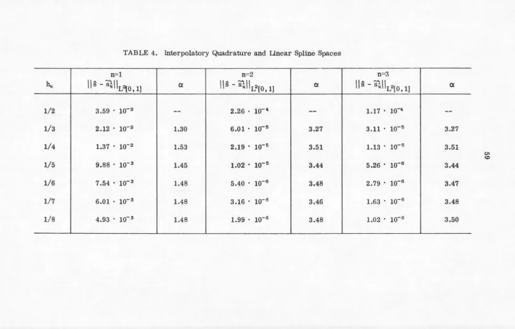
Tables 4, 5, and 6 include, for several values of n, approximate numerical

values for the quantities 11 §N - s~ I IL2[0, 1] where

S?i

is an approximation in

Sp(2m - 1,~N,z), m

=

1,2,m - 1~z~2m - 2, to §N determined by a composit:e

int:erpolatory formula based on n+l-point open Newton-Cotes quadrature formulae.

Again, we include the quantity

a.

The order of accuracy predict:ed by (5.3) as a

n=l n=2

~ _{lls -}

~llv110,11

ex

!Is

-

~llL2[0,

_l] (X

1/2 3.59 • 10-a

--

2.26 • 10-4

--1/3 2.12 • 10-a 1.30 6.01 • 10-5 _3.27

1/4 1.37 • 10-2 _{1.53 2.19 • 10-}5 _3.51

1/5 9.88 . 10-3

1.45 1.02 • 10-5

3.44

1/6 7.54 • 10-3 _{1.48 5.40 • io-}6 _3.48

1/7 6.01 • 10-3 _{1.48 3.16 · 10-}6 _3.46

1/8 4.93 · io-3 _{1.48 1.99 . 10-}6 _3.48

n=3

lls -

~llL2[0,l]

1.17 • 10-4

3.11 · 10-5

1.13 · 10-5

5.26 ' 10-6

2.79 . 10-6

1.63 . 10-6

1.02 · 10-6

(X

--3.27

3.51

3.44

3.47

3.48

3.50

CTI

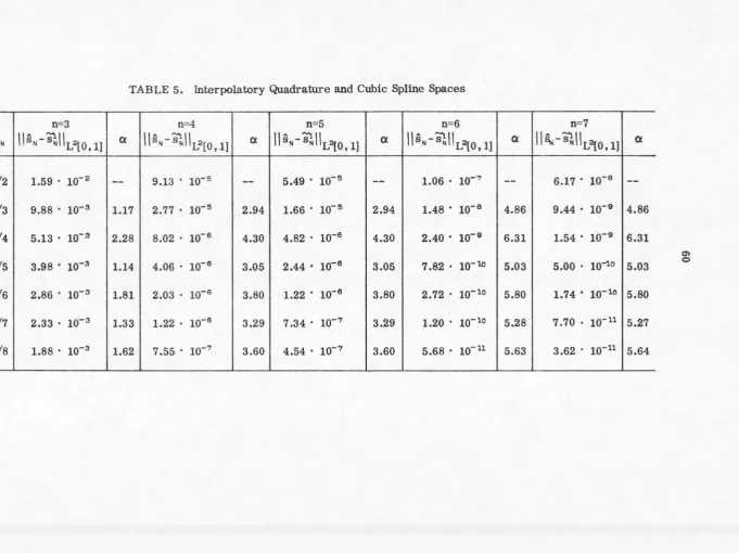
TABLE 5. Interpolatory Quadrature and Cubic Spline Spaces

n=3 n=4 n=5 n=6

bN _{llsN-81llL2(0,1)}

ex

_{11 §N - 81IIL2[0'1]}

ex

_{llsN-8111L2[0,1)}

ex

_{llsN-8111L2(0,1)}

1/2 1.59 . 10- 2

--

9.13 · 10-s

--

5.49 · 10-s

--

1.06 . 10-7

1/3 9.88 . 10-3 _{1.17 2.77 • 10-s 2.94 1.66 • 10-s 2.94 1.48 • 10-e}

1/4 5.13 . 10-3 _{2.28 8.02 · 10-}6

4.30 4.82 • 10-0 _{4.30 2.40 • 10-}9

1/5 3.98 • 10-3

1.14 4.06 · 10-6

3.05 2.44 • 10-6

3.05 7 .82 • 10-10

1/6 2.86 . 10-3 _{1.81 2.03 . 10-}0 _{3.80 1.22 · 10-s 3.80 2.72 . 10-}10

1/7 2.33 . 10-3 _{1.33 1.22 . 10-}0

3.29 7.34 . 10-7

3.29 1.20 . 10-10

1/8 1.88 • 10-3

1.62 7 .55 • 10-7

3.60 4.54 . 10-7

3.60 5.68 • 10-11

n=7

a

ll~-8111L2[0,l]

--

6.17 · 10-e

4.86 9.44 • 10-9

6.31 1.54 • 10-9

5.03 5.00 · 10-io

5.80 1.74 • 10-10

5.28 7.70 . 10-11

5.63 3.62 . 10-11

ex

--4.86

6.31

5.03

5.80

5.27

5.64

n=3 n=4 n=5 n==6

hN

llsN-~llL2[0,1)

a

llsN-~llL2(0,

₁₎

a

llsN-s~lle[o,

11

a

llsN-s~llL2[o,

11

a

1/2 5.9.0 . 10- 2

--

3.82 • 10-4

--

_{2.30 . 10-}4

--

_{4.63 . 10-}7

--1/3 3.62 . 10- 2 1.21 1.05 . 10-4 _{3.19 6.30 ' 10-}5

3.19 5.66 · 10-9 5.19

1/4 2.60 . 10- 2 1.15 4.26 · 10-s 3.13 2.56 · 10-5 _{3.13 1.29 · 10-}9 _5.13

1/5 2.03 · 10- 2 1.12 2.13 · 10-5

3.11 1.28 • 10-5 _{3.11 4.14 • 10-}9 _5.11

1/6 1.66 · 10- 2 1.11 1.21 • 10-5 3.10 7.26 · 10-s 3.10 1.63 • 10-9 _5.10

1/7 1.40 · 10-2 1.09 7.51 · 10-s 3.09 4.51 · 10-6 _{3.09 7.46 . 10-}10 _5.09

1/8 i.21 · 10- 2 1.09 4.98 • 10-e 3.08 2.99 · 10-s 3.08 3.78 . 10-10 _5.09

n=7

I

I

SN-

~I

IL2[0, 1]

2.96 . 10-7

3.61 · 10-9

8.26 • 10-9

2.64 • 10-9

1.04 . 10-9

4. 76 · 10-10

2.41 . 10-10

a

--5.19

5.13

5.11

5.10

5.09

5.09

O'l

62

discrepancies between the observed and predicted values of the order of

accu-racy of this technique in the L2_{-norm. For the linear spline spaces, Sp(l, AN, 0),}

we observe the values of 1.5, 3.5, and 3.5 for the limiting values of

a

when

n

=

1, 2, and 3, respectively, and yet the values predicted by the theoretical

resuits are 0.5, 1.5, and 2.5. We observe, however, that special error bounds

can be derived for odd point (even values of n) Newton-Cotes formulae which

yield an additional order of accuracy. Consequently, we observe a constant

discrepancy of one between the predicted and observed orders of accuracy in

approximating the least square linear spline approximation to the exponential

function using this type of discretized technique. We note that the corresponding

table in the L co -norm reflects the loss of a half of an order of accuracy predicted

by theoretical considerations. However, we have not included this table in this

presentation of our numerical results. In the cubic case, i.e., m

=

2 and z

=

2,

we observe the numbers of 1.5, 3.5, 3.5, 5.5, and 5.5 for the limiting values of

a

when n = 3, 4, 5, 6, and 7 and again find discrepancies with the predicted values

of 0.5, 1.5, 2.5, 3.5, and 4.5. Considering the additional order of accuracy for

odd point Newton-Cotes formulae, we again observe a constant discrepancy of one

order of accuracy between the computed and predicted values of

a.

We also note

that a predicted loss of a half an order of accuracy can be observed when the

corresponding table in the Leo-norm is computed. Finally, for the cubic Hermite

spline spaces, i.e., m = 2 and z = 1, the observed values of

a

are tending to

1.0, 3.0, 3.0, 5.0, and 5.0 for n = 3, 4, 5, 6, 7 and the predicted values based on

5.5, and 5.5 just as in the cubic case. However, here we observe the constant

discrepancy of one half of an order of accuracy between the predicted and observed

values for

a..

In this case, the loss of a half order of accuracy predicted by theo-retical considerations when using La-error bounds and Sobolev type inequalities

to generate L

=

error bounds is not observed. These same discrepancies were

observed in least square approximation of the function sin (2x), 0 s: x s: 1. The

analogous tables for the Filon type quadrature schemes show no discrepancies

between the predicted and observed values of ex. Consequently, we omit them

from this presentation of numerical results.

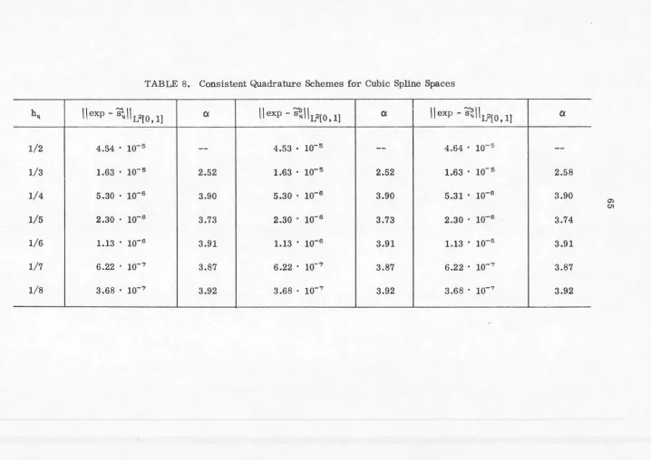
Corresponding to the spline spaces Sp(l,A,.,O), Sp(3,Ai,2), and Sp(3,~,1),

respectively, in Tables 7, 8, and 9, we present approximate numerical values

for the quantities \\exp -

~\\V'{O,

l]' \\exp -

s~llL2[0,

l]' and !lexp -

s~l\Vl[O,

l]

where the quadrature schemes used to determine the discretized spline

approxi-mations are chosen to be consistent with the L2-bounds for the least square error

as given by (5.1). Specifically, the composite interpolatory formula employed to

determine $1£ Sp(2m - 1,AN,z) is based on (4m - 1) - pt open ended Newton-Cotes

formulae and the Filon scheme used to determine s~ is based on piecewise Lagrange

interpolation of degree 2m - 1. For any fixed value of N, the data points used to determine the approximations are the same for each technique. Again the quantity,

ex, as defined in previous tables is included. We note that both discretized

approxi-mations, ~and~. exhibit the consistent behavior predicted by our theoretical

considerations. We also note that the standard discrete least square technique

TABLE 7. Consist.ent Quadrature Schemes for Linear Spline Spaces

hN

_{\\exp -}

~\IL2[0,

1]

ex

\\exp -

~I

IL2[0, 1]

ex

\\exp -

s~\\L2[0,

1]

1/2 1.68 . 10- 2

--

1.72 . 10- 2

--

1.69 . 10-2

1/3 7.48 . 10-3 _{2.01 7.62 . 10-}3 _{2.00 7.5}