Volume 2008, Article ID 497187,10pages doi:10.1155/2008/497187
Research Article
Achievable ADC Performance by Postcorrection Utilizing
Dynamic Modeling of the Integral Nonlinearity
Niclas Bj ¨orsell1and Peter H ¨andel2
1ITB/Electronics, University of G¨avle, 801 76 G¨avle, Sweden
2Signal Processing Lab., ACCESS Linnaeus Center, School of Electrical Engineering, Royal Institute of Technology, 100 44 Stockholm, Sweden
Correspondence should be addressed to Niclas Bj¨orsell,[email protected]
Received 1 May 2007; Revised 24 September 2007; Accepted 19 December 2007
Recommended by Boris Murmann
There is a need for a universal dynamic model of analog-to-digital converters (ADC’s) aimed for postcorrection. However, it is complicated to fully describe the properties of an ADC by a single model. An alternative is to split up the ADC model in different components, where each component has unique properties. In this paper, a model based on three components is used, and a performance analysis for each component is presented. Each component can be postcorrected individually and by the method that best suits the application. The purpose of postcorrection of an ADC is to improve the performance. Hence, for each component, expressions for the potential improvement have been developed. The measures of performance are total harmonic distortion (THD) and signal to noise and distortion (SINAD), and to some extent spurious-free dynamic range (SFDR).
Copyright © 2008 N. Bj¨orsell and P. H¨andel. This is an open access article distributed under the Creative Commons Attribution License, which permits unrestricted use, distribution, and reproduction in any medium, provided the original work is properly cited.
1. INTRODUCTION
The analog to digital converter (ADC) is a key component in many applications, for example, radio base stations and test and measurement instruments. In state-of-the-art de-signed vector signal analyzers (VSAs), the ADC is the bot-tle neck and an improvement in ADC performance directly improves the VSA performance. Characterization and test-ing of ADC’s are important in many different aspects. One example is ADC postcorrection, where improvements in the ADC characteristics are obtained by digital signal process-ing methods, in particular the error occurrence is predicted in order to compensate for error source effects. A survey of error compensation methods is given in [1]. Postcorrection is built on the model of the ADC. A survey of state-of-the-art ADC modeling techniques and models may be found in [2]. Normally, the ADC model is based on a characteriza-tion performed in high-performance test setups, whereupon an off-chip postcorrection algorithm is developed. In the lit-erature, a majority of the proposed ADC characterization methods describes the static properties of the converter. A common solution for postcorrection based on a static model is the use of lookup tables (LUTs); that is, the ADC output
is remapped using a table lookup, where the table entries are such that some performance measure is improved, as for example [3]. ADC postcorrection by table lookup methods has shown to improve performance measures such as spuri-ous free dynamic range (SFDR), total harmonic distortion (THD), and signal-to-noise and distortion ratio (SINAD). It has been shown that postcorrection based on LUTs that do not take the dynamics of the ADC into account is band limited (see, e.g., [4,5]). Characterization and testing of the dynamic effects of ADC’s are instrumental for the perfor-mance of systems characterized by a wide bandwidth and high-dynamic range, such as contemporary and future mo-bile telephony systems requiring higher resolution and sam-pling rates.
ADC Inversemodel
v(t)
k(n)
k(n−d)
v(n) .
. .
Figure1: Postcorrection by using an inverse model of the ADC.
flexibility between the dynamics (i.e., the number of delayed samples) and the precision or number of bits of each sample. Thus, the size of the multidimensional lookup table is kept at a reasonable predetermined number. However, these meth-ods are burdensome considering the time they take to train the entries of the LUT, as well as the requirement on the size of the memories. Accordingly, there is a need for dynamic postcorrection that is easy to train and simple to implement. A parametric model requires less memory size than an LUT and does not need to be trained for every combination of present and previous samples. A well-assigned model is able to describe scenarios for which it is not trained, even though one should strive to train the model with a stimulus as realistic as possible for a given application. Different types of parametric models have been suggested in the literature, such as Volterra models and a variety of different box models (e.g., Wiener and Hammerstein models). These models de-scribe the nonlinear dynamic behavior well, but typical error models of an ADC also include components that can not be described by nonlinear dynamic models. That implies that a postcorrection that compensate for multiple kinds of er-ror behavior might be based on two or more models, where each error behavior is compensated with a suitable postcor-rection method. The purpose of this paper is to provide a tool to evaluate to what extent a given parametric model can improve the ADC performance, when the model is used for postcorrection.
Postcorrection can be divided into two different meth-ods. One method is to use an inverse ADC model and the other is to add a correction term. When using LUT for post-correction, the two methods are often denotedreplacement
andcorrection, respectively. The inverse model corresponds to replacement. The output code from the ADC is a table in-dex. The code addresses a memory, where the memory value of that address is an estimate of the analog input. The index can also be compounded by one or more previous samples (seeFigure 1).
Figure 1can also represent a correction method based on inverse models. In other words, the method is based on some mathematical system model and its inverse. Typically, a model is characterized for the ADC under test. The model gives an approximation of the input-output signal relation-ship. An inverse—possibly approximate—of the model is cal-culated, thereafter. The model inverse is used in sequence af-ter the ADC, hence operating on the output samples, in order to reduce or even cancel the unwanted distortion.
Instead of replacing the output code from the ADC, one can add a correction term. (seeFigure 2). In postcorrection using LUT, the output sample (possibly together with previ-ous samples) addresses a correction term instead of an
esti-G v(t)
ADC
v(n)
INL[k,ω] INL[k,ω]
Postcorrection
k[n]
Figure2: Postcorrection of an ADC by adding a correction term. The blockGincludes analog preprocessing, sample and hold, and quantization.
0 1 2 3 4 5 6 7
Vmin
Output
dig
ital
co
de
k
0
Analog inputV(Volt)
Vmax
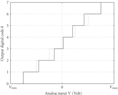
Figure3: The relationship between the analog input signalvand the digital output codekfrom an idealn = 3 bits ADC (dashed line) and a practical one (solid line).
mate of the input as in the replacement method. The cor-rection term is added to the output code. In model-based postcorrection, the postcorrection term is computed from a mathematical model. The correction term is added to the output code. In a static postcorrection, the correction term corresponds to the ADC integral nonlinearity (INL).
2. BASIC PROPERTIES OF ADC NONLINEARITIES
The relationship between the analog input signal V [Volt] and the digital output codek from an ideal ADC approxi-mates the dotted staircase transfer curve shown inFigure 3. For the ideal ADC, the code transition levelsTk[Volt] within
the ADC range (Vmin,Vmax) [Volt] are given by
Tk=Q(k−1) +T1[Volt], (1)
where Q [Volt] is the ideal width of a code bin; in other words, the full-scale range of the ADC is divided by the to-tal number of codes (Vmax−Vmin)/2N, whereNdenotes the number of bits. Further,T1is the ideal voltage correspond-ing to first transition level, andT1 is equal toVmin+Qor
Vmin +Q/2 depending on the convention used: the “mid-riser” convention or “mid-tread” convention, respectively [10]. The codekspansk=1,. . ., 2N−1.
−1 −0.8 −0.6 −0.4 −0.2 0 0.2 0.4 0.6 0.8 1
INL
[LSB]
0 500 1000 1500 2000 2500 3000 3500 4000 Transition level [LSB]
Figure4: Exemplary measured INL from a 12 bit commercial ADC.
by the solid line inFigure 3. The actual code transition level
T[k] [Volt] (i.e., the ideal and practical transition levels are distinguished by the placement of the argumentk, viz.Tkand
T[k], resp.) is the voltage that results in a transition from ADC output code k−1 to k. The INL is described as the difference between the idealTk in (1) and the actual T[k]
code transition levels of the ADC, after a correction has been made for gain and offset errors [10,11]. Given the ideal code transition levelsTkin (1) and the measured levelsT[k], the
correction is made by adjusting the gainGand offsetVosin order to “minimize” the residualε[k] (fork=1,. . ., 2N−1)
[10],
ε[k]=Tk−G·T[k]−VOS[Volt]. (2)
Equation (2) describes an overdetermined set of 2N−1
equa-tions with the two unknownsGandVosthat are sought for. According to the IEEE standards [10], different methods may
be applied for determining the optimal (G,Vos)-pair such as the “terminal-based” method [10] as used in this paper. The INL as a percentage of the full scale (FS) range of the ADC is given by the normalized residual in (2), that is,
INL[k]=100%·ε[k]
2NQ [% of FS]. (3)
The INL is normally expressed in least significant bits (LSBs), where a LSB is synonymous with one ideal code bin widthQ
[Volt], that is, INL[k]=ε[k]/Q[LSB].
Differential nonlinearity (DNL) is the difference, after correcting for the obtained static gainG, between a speci-fied code bin width and the ideal code bin widthQ, divided by the ideal code bin width. The DNL is given as follows:
DNL[k]=W[k]−Q
Q [LSB], (4)
where W[k] is the corrected width of code bin k, that is,
W[k] = G(T[k + 1] −T[k]). From (2), it follows that
ε[k+ 1]−ε[k]=Q−W[k], and thus the relation between INL[k] and DNL[k] is
DNL[k]=INL[k+ 1]−INL[k]. (5)
The root-mean-square (RMS) value of the DNL is commonly used and given by
DNLRMS=
1 2N−1
2N−1
k=1
DNL2[k] 1/2
. (6)
3. PARAMETRIC INL MODELING FOR ADC POSTCORRECTION
In Figure 4, a typically measured INL from a commercial ADC is plotted. As it is evident from the plot, the behav-ior is a combination of a smooth wave or polynomial curve and a prickly sawtooth wave. In the following analysis, the INL will be broken up in two components; one representing the smooth curve and one representing the prickly sawtooth wave. The INL[k] is then described as
INL[k]=HCFINL[k] +LCFINL[k], (7)
where the first term is the contribution by the, so-called, high-code frequency component and the second term by the low-code frequency component, respectively. In [12], the static INL model was expressed as a one dimensional image in the codekdomain consisting of the two components. The smooth curve was entitled low-code frequency (LCF), to un-derstand the meaning of low-frequency code, consider that the code axis represent a time axis. Accordingly, low-code fre-quency means slow variation over the codes, [13] component denoted byLCFINL[k] and was represented by a polynomial approximation:
LCFINL[k]=h
0+h1k+h2k2+· · ·hLkL, (8)
where the hk’s are the polynomial coefficients and Lis the
order of the polynomial. The parametersh0andh1are typ-ically set to zero due to the fact that INL is calculated after a correction has been made for gain and offset errors when determining the INL [10]. The high code-frequency compo-nentHCFINL[k] is caused by a significant deviation between
the polynomial approximation (8) and the actual INL[k]. In [14], the high-code frequency component was further divided into two parts:HCFINL[k] andNoiseINL[k], respec-tively. The former term,HCFINL[k], depends on the physical design of the component (designs such as pipeline, succes-sive approximation, or any other structure) and is modeled as piecewise linear [12,15]. The latter component,NoiseINL[k], is the part of INL[k] that cannot be described by an equation. Thus, the INL[k] model in (7) is refined to
INL[k]=HCFINL[k] +LCFINL[k] +NoiseINL[k]. (9)
A static model of an ADC and in particular the correspond-ing INL[k] is in general not sufficient to accurately describe
done by adding amplitude information from either previous sample amplitudes or estimates of the input slope, which is state-space and phase plane modeling, respectively. The dy-namic behavior of the INL can alternatively be described as a frequency dependency, that is, different sine wave test stimuli result in different INL data. One may note that frequency se-lective LUTs for ADC postcorrection was considered in [16]. In order to stress the dependency of some of the components in (9) on the stimuli frequencyω, (9) is rewritten as
INL[k,ω]=HCFINL[k] +LCFINL[k,ω] +NoiseINL[k,ω], (10)
whereωdenotes the normalized frequency variable,
ω= 2π f
fs
, (11)
where f is the actual frequency in Hertz and fsis the
sam-pling frequency.
The main purpose of the model (10) is to use it for ADC postcorrection. The structure of the components of the model may, to some extent, be affected by the aim to find a dynamic model that is easy to train and simple to implement. Even though the behavior models are black-box mod-els, the arguments for having a staticHCFINL[k] can be jus-tified based on some knowledge of the ADC design. The hardware structure of an ADC is consisting of two sections. First is an analog signal processing section with an ampli-fier and sample-and-hold circuits followed by a section per-forming the quantization. The high-code frequency compo-nentHCFINL[k] is mainly representing the imperfections in the quantizer, which are (at least in a first approximation) static and thus depend on the codek only and not on the test frequency. One favorable feature with considering the high-code frequency component to be static is that the size of the lookup table will be minimized. The low-code fre-quency componentLCFINL[k,ω] is a two-dimensional para-metric model describing a dynamic behavior. Due to the pa-rameterization, the postcompensation can be implemented by numerical calculations.
The componentLCFINL[k,ω] is described as a nonlin-ear dynamic model and can be described by different model structures. In [17], the input-output relation of the ADC was explored based on measured Volterra kernels [18]. In partic-ular, in that paper it was argued for employing a constrained nonlinear Volterra model known as the parallel Hammer-stein model [19]. Based on the promising results in [17], the parallel Hammerstein model is used in this work to analyze the nonlinear dynamic parts of the integral nonlinearity, as well. The basic Hammerstein model is given by a static non-linearity, followed by a linear filter. The difference between the ordinary Hammerstein model and the parallel structure is that the contributions of different orders l are now fil-tered by different filters defined by their frequency functions Hl[ω], respectively. Starting with the polynomial nonlinear-ity i (8), a frequency dependency is incorporated by letting the polynomial coefficient be frequency dependent, that is,
LCFINL[k,ω]=h0(ω) +h1(ω)k+h2(ω)k2+· · ·+h
L(ω)kL.
(12)
The above dynamic nonlinearity can be described in terms of a parallel Hammerstein model with thelth single-input multiple-output given bykl, and the zero phase linear filters with frequency functionhl(ω). In summary, the
paral-lel Hammerstein structure with a polynomial nonlinearity is a natural generalization of the static polynomial model (8). Although in this paper constraints are imposed both on the static nonlinearity as well as the phase characteristics of the bank of linear filters, the obtained dynamic model will be used throughout this paper in order to analyze and compen-sate for the nonlinear dynamic parts of ADC integral nonlin-earity.
TheLCFINL[k,ω] is a continuous function by construc-tion and thus models employing Volterra Kernels or a box-model for the transfer function are appropriate. Moreover, the noncontinuous behavior is modeled by the remaining terms, that is, HCFINL[k] and NoiseINL[k,ω], respectively. The complete block scheme over the employed dynamic INL model is given inFigure 5. The high-code frequency compo-nentHCFINL[k] depends on the codekonly, and not on the test frequency. Further,HCFINL[k] is as in [15] assumed to be piecewise linear in the codek; in other words, it is described by the first-order polynomialα0+α1kwithin a limited set of neighboring code valueskp−1≤k < kp; denoted as the code
intervalKp. TheHCFINL[k] is thus modeled such that
HCFINL[k]=α0[p] +α1[p]k−k
p−1
, (13)
whereprefers to the ordered code interval
Kp: k|kp−1≤k < kp
, (14)
wherep=1,. . .,P. The initial value ofk0is given byk0=1, and the upper end point is, by definition,kP=2N. Typically,
the number of intervalsP is small compared with the total number of codes,P2N−1 (see, e.g., the INL curve given
inFigure 3).
Two different postcorrection methods based on the theo-ries given inSection 3were presented in [14,20], respectively. In both papers, the different componentsLCFINL[k,ω] and HCFINL[k] were postcorrected separately and the dynamics were concentrated to the low-code frequency component.
4. IDENTIFICATION OF INL MODEL PARAMETERS FROM MEASUREMENTS
In [15], the dynamic characterization of an ADC, when us-ing a plurality of different test frequencies in the measure-ment setup, was considered. In particular, the different test frequencies are denoted by the integerm, that is, a one-to-one map to the employed set of test frequencies f1· · ·fMin
Hertz. This ordering of test frequencies attaches the notation, that is, the normalized frequencyωis below replaced by the integermcorresponding to the actual test frequency fm (in
Hertz).
k[n]
α0[1] +α1[1](k−k0)
α0[2] +α1[2](k−k1)
α0[p] +α1[p](k−kp−1)
. . .
N[·]
k2[n]
kL[n]
. . .
NoiseINL
h2(ω)
hL(ω)
. . .
+
+ +
LCFINL INL
HCFINL
HCFINL
k∈kp
Figure5: A block scheme over the complete INL model. The nonlinear blockN[·] is a polynomial.
measurements. A closed-form solution to the estimation problem was derived. The method in [15] is reviewed be-low. The high-code frequency component is assumed to be piecewise linear in the codek, that is, described by (13) and (14). Accordingly, there arePsets of polynomial coefficients
{α0[p],α1[p]}, which are gathered in the parameter vectorη of size 2P. That is,
η=
⎛ ⎜ ⎜ ⎜ ⎜ ⎜ ⎜ ⎝
α0[1]
α1[1] .. .
α0[P]
α1[P] ⎞ ⎟ ⎟ ⎟ ⎟ ⎟ ⎟ ⎠
. (15)
The parameter vectorηin (15) describes the local gain and offset in INL for the different code intervals Kp. As
pre-viously mentioned, the high-code frequency component is, at least approximately, independent of the input test fquency. The low-code frequency component models the re-maining dynamic behavior of the INL. The latter component LCFINL[k,ω] is modeled by a polynomial of order L as in
(12). Consider the signal model
LCFINL[k,m]= f[k]T
θ[m], (16)
where T denotes transpose. In (16), the vector θ[m] =
h2[m] · · · hL[m]
T
is the parameter vector (i.e.,θ[m] is possibly dependent on the test frequency as indicated by the
argument m) and f[k] = k2 · · · kLT is the regressor.
One may note that each entry in the parameter vector de-scribes the gain of the corresponding zero-phase filter in the parallel Hammerstein model. In order to estimate the pa-rameters in the dynamic model of the integral nonlinear-ity, experiments are performed where in each experiment a sinewave Histogram test is used in order to pick up a set of INL data. Collecting all experimental data corresponding to the unique test frequency fm[Hertz] in an vectorym, a least
squares fit is employed in order to fit the model parameters,
so that ym is as close as possible (in least squares) to our
model, that is,
ym=
⎛ ⎜ ⎜ ⎝
INL[1,m] .. . INL2N−1,m
⎞ ⎟ ⎟
⎠, m=1,. . .,M. (17)
In (17),ymis the vector with experimental data and the
right-hand side in our model (10), where the frequency vari-able used in (10) has been replaced by its corresponding in-teger valuem.
We introduce (wherepspansp=1,. . .,P)
gp=
⎛ ⎜ ⎜ ⎝
1 0
..
. ... 1 kp−kp−1−1
⎞ ⎟ ⎟
⎠ (18)
with the convention thatk0 = 1 andkP =2N. Further, we
introduce the Vandermonde matrixfof size 2N−1×L+ 1
given by
f=
⎛ ⎜ ⎜ ⎝
10 11 · · · 1L
..
. ...
2B−10 2B−11 · · · 2B−1L
⎞ ⎟ ⎟
⎠. (19)
Then we may put the model that describes the experimental integral nonlinearity on a vector form as
ym=gη+kθ[m] +em, (20)
whereηis given by (15). Here,gis introduced as the block diagonal matrix with thegp’s defined by (18) on its main
di-agonal, that is,g=blockdiag(g1,. . .,gp).
{y1,. . .yM}and expanding the parameter vector with them -dependent components, that is,
⎛ ⎜ ⎜ ⎝
y1 .. . yM
⎞ ⎟ ⎟ ⎠
y
=
⎛ ⎜ ⎜ ⎝
g f .. . . ..
g f
⎞ ⎟ ⎟ ⎠
[GF] ⎛ ⎜ ⎜ ⎜ ⎜ ⎝
η θ[1]
.. .
θ[M] ⎞ ⎟ ⎟ ⎟ ⎟ ⎠
⎡ ⎣η
θ ⎤ ⎦
+ ⎛ ⎜ ⎜ ⎝
e1 .. . eM
⎞ ⎟ ⎟ ⎠
e
. (21)
The least-squares (LS) solution of (21) is by a block ma-trix notation given by
η
θ
=
GT
FT G F −1
GT FT
y. (22)
In [15], it is shown that the above LS solution can be sepa-rated into one solution forηand one for each of theM fre-quency independent parameter vectorsθ(m). The complex-ity of the LS solution is significantly reduced by exploiting the spares structure of the involved matrices, leading toM+1 sets of solutions, that is,
η=gTπ⊥g
−1
gTπ⊥y, (23)
θ[m]=fTf−1fTym−gη
, m=1,. . .,M. (24)
In (23),yis defined as the average (over all test frequencies) of all INL data, that is,
y= 1
M
M
m=1
ym. (25)
Further,π⊥is given by
π⊥=I−ffTf−1fT, (26)
whereIdenotes the unity matrix of proper size.
We note that (23) is a linear combination of the averaged INL data (25). Regarding (24), one may note that this is the least-squares solution corresponding to the detrended data ym−gη.
5. PERFORMANCE ANALYSIS
The purpose of postcorrection is to improve the perfor-mance for the system, where the ADC’s are used. Commonly used figures of merits are THD, SFDR, and SINAD. For a model-based postcorrection based on the model structure described in Section 4, and given that all model parame-ters are estimated, questions of relevance include the follow-ing. What are the achievable performance improvements for these figures of merits? How advanced must the postcorrec-tion method be to meet the demands for the system?
InSection 5.1, we will formulate the relationship between a given INL model and the ADC performance, hence, the po-tential of improvement of an optimal postcorrection. Below, the influence of the three terms in (10) on the ADC per-formance measures are investigated separately. By gradually
correcting for each INL term, the performance will improve step by step. We consider the case when a multiterm dynamic model of the INL (such as (10) above) is available, and is used for postcorrection as illustrated inFigure 2.
The termNoiseINL[k,ω] in (10) is throughout the paper modeled as noise, so thatNoiseINL[k,ω]=e[k,ω] is assumed to be zero mean independently identically distributed noise both in the codekand in test frequencyω. The general rela-tion (10) is accordingly reduced to
INL[k,ω]=LCFINL[k,ω] +HCFINL[k] +e[k,ω]. (27)
In the following sections, we will describe the different components in more detail and how they affect the perfor-mance of the ADC. The conditions for the analysis are that the ADC performance is limited by the effects of the inte-gral nonlinearity. In the following analysis, an expression for the THD, SINAD (and to some extent also the SFDR) as functions of the INL model parameters is developed. Con-sequently, the derived expressions constitute an upper limit on the performance improvements by postcorrection elim-inating the effects of INL. That is, under the condition that the estimated INL used for postcorrection corresponds to the actual INL of the ADC.
5.1. Effects of the INL low-code frequency component
on ADC performance
The LCFINL[k,ω] is a weakly nonlinear dynamic transfer function (12). Since its transfer function is a polynomial, LCFINL[k,ω] will mainly affect the harmonic distortion such
as THD, and also SFDR since the 2nd and 3rd harmonics are usually the limiting spurs in SFDR. To get a measure on how the ADC performance depends on this component, an eval-uation in the frequency domain will be done.
For simplicity, but without loss of generality, the analysis is performed in continuous time. Let the time domain input
v[t] to a static nonlinear system with outputx[t] be a unit amplitude cosine with zero initial phase
v[t]=cosω0t= e
jω0t+e−jω0t
2 , (28)
wheretis the absolute time, and jis the imaginary unit j = √
−1. The harmonic distortion on the outputx[t] of a static nonlinearity driven by inputv[t] is given by a combination of (28) and (12), that is,
x[t]=h0+h1e
jω0t+e−jω0t
2 +h2
ejω0t+e−jω0t
2
2
+· · ·+hL
ejω0t+e−jω0t
2
L
.
(29)
Note that, we here includeh0 andh1 since the output from the ADC is a sum of a linear quantization of the input
v[t] (whereh0andh1are included) and the nonlinear error model given by INL[k,ω] (i.e., described byh2(ω)· · ·hL(ω)
The even exponents produce harmonic distortion prod-ucts at the ADC level and on even multiples of the funda-mental frequency. Odd exponents will result in distortion at odd overtones. For example, the third-order component reads
h3
ejω0t+e−jω0t
2
3
=h3
ej3ω0t+e−j3ω0t+ 3ejω0t+e−jω0t
8
=h3 !
1
4cos 3ω0t+ 3 4cosω0t
"
.
(30)
In a more general case of ordern, one can find the coeffi -cients from the binomial theorem,
(c+d)l=
l
i=0
l
i
cl−idi. (31)
For example, the outputvl[t] will have the following set of frequencies:
vl[t]=
⎧ ⎪ ⎪ ⎪ ⎪ ⎪ ⎪ ⎪ ⎪ ⎪ ⎪ ⎪ ⎪ ⎪ ⎪ ⎪ ⎪ ⎪ ⎪ ⎪ ⎪ ⎨ ⎪ ⎪ ⎪ ⎪ ⎪ ⎪ ⎪ ⎪ ⎪ ⎪ ⎪ ⎪ ⎪ ⎪ ⎪ ⎪ ⎪ ⎪ ⎪ ⎪ ⎩ 1 2l−1
l
i=1
1−(−1)i 2
⎛ ⎜ ⎝ i−l1
2 ⎞ ⎟ ⎠
×cos(l−i+ 1)ω0t
l odd,
1 2l−1
⎛ ⎜ ⎝1 2 ⎛ ⎜ ⎝ ll
2 ⎞ ⎟ ⎠+
l−2
i=0
1 + (−1)i 2
×
⎛ ⎜ ⎝ li
2 ⎞ ⎟
⎠cos(l−i)ω0t
⎞ ⎟
⎠ l even.
(32)
The componentsvl[t] are the input to the linear parts of the parallel Hammerstein model, where each branchvl[t] will be filtered by the corresponding zero-phase linear filter. The re-sulting output of the parallel Hammerstein modely[t] reads
y[t]=A0+A1cos
ω0t
+A2cos
2ω0t
+· · ·+ALcos
Lω0t
, (33)
where the real-valued A-coefficients are obtained from fil-tering the componentsvl[t] given in (32) by the individual zero-phase filters in the parallel Hammerstein model
A0= 1 22 2 1
h2(0) + 1 24
4 2
h4(0) +· · ·, (34)
A1=h1 ω0 + 1 22 3 1 h3 ω0 + 1 24 5 2 h5 ω0 +· · ·, (35)
A2= 1
21 2 0 h2
2ω0 + 1 23 4 1 h4
2ω0
+· · ·, (36)
A3= 1
22 3 0 h3
3ω0 + 1 24 5 1 h5
3ω0
+· · ·. (37)
For an arbitrary orderq, one has
Aq=
⎧ ⎪ ⎪ ⎪ ⎪ ⎪ ⎪ ⎪ ⎪ ⎪ ⎪ ⎨ ⎪ ⎪ ⎪ ⎪ ⎪ ⎪ ⎪ ⎪ ⎪ ⎪ ⎩ L
i=q
1 + (−1)q 2
1 2i−1
⎛ ⎜ ⎝ i−iq
2 ⎞ ⎟ ⎠hi
qω0 qeven, L
i=q
1−(−1)q 2
1 2i−1
⎛ ⎜ ⎝ i−iq
2 ⎞ ⎟ ⎠hi
qω0
qodd.
(38)
For a pure sinusoidal input signal, the amplitudeA1is the fundamental tone and allAq, whereq /=1, are distortion
prod-ucts. Thus, the figure of merit THD (and eventually SFDR) can be expressed as a function of the amplitudes, as outlined below.
5.1.1. Total harmonic distortion (THD)
For a pure sinewave input of a specified amplitude and fre-quency, the THD is the root sum of squares (RSS) of all the harmonic distortion components including their aliases in the spectral output of the ADC. Normally, THD is estimated by the RSS of the second through the tenth harmonics, in-clusive. THD is often expressed as a dB ratio with respect to the root mean square (RMS) amplitude of the output com-ponent at the input frequency.
The total harmonic energy (THE) for the specific subset of harmonics is defined by [10]
THE= 1
R2
n
''Y
ωn''
2
, (39)
whereRis the length of the data record,Y[ωn] is the complex
value of the spectral component at frequencyωn. Further,ωn
is thenth harmonic frequency of the discrete Fourier trans-form (DFT) of the ADC output data record,Mis the number of samples in the data record, andnis the set of harmonics over which the sum is taken. The absolute value ofY[ωn] is
the amplitudeAn.
Employing the above expression for theLCFINL, the result reads
LCFTHE= 1
R2
L
l=2 ''Y
ωl''2= 1
R2
L
l=2
A2
l, (40)
whereLis the order of the polynomial in (12).
The total harmonic distortion is given by the ratio THD=√THE/A1. The THD is often expressed as a dB ratio with respect to the RMS amplitude of the fundamental com-ponent of the output. The maximum achievable gain in the postcorrection of the ADC is accordingly given by the total harmonic distortion from the low-code frequency compo-nent,
LCFTHD=20 log 10
!√LCF THE
A1 "
. (41)
5.1.2. Spurious-free dynamic range (SFDR)
level of the largest spurious or harmonic component for a large, pure sinewave signal input. Including harmonics re-flects common usage of the term SFDR. Normally the second or third harmonic in (36) or (37) will be the limiting spuri-ous. Under condition that postcorrection can eliminate these harmonics, the SFDR will be limited by a nonharmonic or high-order harmonic distortion. An exact values for achiev-able performance it thus not possible to find.
5.1.3. Signal to noise and distortion ratio (SINAD)
The signal-to-noise-and distortion ratio (SINAD) is the ratio of the signal to the total noise. Unless otherwise specified, it is assumed to be the ratio of RMS signal to RMS noise, in-cluding harmonic distortion, for sinewave input signals [10]. To study the effects ofLCFINL, SINAD is evaluated in the fre-quency domain.
Both the signal and the total noise can be determined from the DFT of data records. LetEavm[ω] equal the resid-ual spectrum ofYavmafter the bins atωm=0 (DC) and test
frequencies, ω0, have all been set to zero (excised from the spectrum). Then, the RMS noise is found from the sum of all the remaining Fourier components,
rms noise= 1
R
M−1
m=0 ''Eavm
ωm''2
1/2
. (42)
The contribution to the noise fromLCFINL[k] isLCFTHE. The noise will thus be reduced to
rms noise= 1
R
M−1
m=0 ''
Eavm
ωm''2−LCFTHE
1/2
. (43)
To conclude this section, the achievable effect from elim-inating the low-code frequency component by using postcor-rection is for THD given by (41) and for SINAD by (43). In indication of potential, SFDR improvement is given by (38), if the limiting spurious is an overtone.
5.2. Effects of the high-code frequency component on
ADC performance
Since both THD and SFDR are evaluated in the frequency domain, these components can be described by a transfer function with an amplitude dependent piecewise constant amplification. How this will affect the harmonic distortion can be found from its DFT, where the error fromHCFINL[k] will result in a piecewise constant amplification:
yHCF(t)= ⎧ ⎪ ⎪ ⎪ ⎪ ⎪ ⎪ ⎨ ⎪ ⎪ ⎪ ⎪ ⎪ ⎪ ⎩
α1sin(ωt) +O1 sin(ωt)< k1,
α2sin(ωt) +O2 k1≤sin(ωt)< k2, ..
. ...
αPsin(ωt) +Op kP−1≤sin(ωt),
(44)
whereOis an offset and yHCF(t) is an virtual, internal signal in the INL model (Figure 5), namely, theHCFINL output for a single tone stimulus.
The harmonic distortion is highly dependant on the structure of HCFINL[k] given in (13). Thus, one needs to solve and the DFT for (44) for the specific ADC used to get information about the effects on the THD and SFDR. How-ever, one property of HCFINL[k] worth mentioning is that the amplitudes from the harmonics fromHCFINL[k] are not necessarily declining with the order of the harmonic. For a smooth nonlinearity (as in the low-code frequency compo-nent) the amplitude of harmonics decreases with higher or-der, but this not necessarily the case forHCFINL[k].
Since we are not able to find a general expression for the effect fromHCFINL[k] in the frequency domain, we will eval-uate SINAD based on the results from [21], where the max-imum achievable SINAD for aN-bit ADC is for a floating-point postcorrection given by
SINAD= 2
2N
1 + 3·DNL2RMS, (45)
where DNLRMSwas defined in (6). In [22], (45) was further developed to include a correction algorithm with a fixed-point resolution for correction values.
Assume that we have eliminated the errors due to the low-code frequency component. That will give us from (27) the remaining INL[k] to beHCFINL[k],
HCFINL[k]=HCFINL[k] +e[k]. (46)
The differential nonlinearity DNL[k] is found from (5), that is,
DNL[k]
=HCFINL[k+ 1]−HCFINL[k] =e[k+ 1]−e[k]
+ ⎧ ⎪ ⎪ ⎪ ⎨ ⎪ ⎪ ⎪ ⎩
α1[p] kp−1< k < kp
α0[p]−α0[p−1]−α1[p−1]k−1−kp−2
k=kp−1. (47)
Since{e[k]}are random variables independent and identi-cally distributed, DNL2RMSyields
DNL2RMS
= 1
2N−2
2N−2
k=1
DNL2[k]
= 1
2N−2
2N−2
k=1
ErrorDNL2[k]
+ 1
2N −2 P
p=1 !
α1[p]2kp−kp−1
+ α0[p]−α0[p−1]−α1[p−1]kp−1−1−kp−2 2"
,
whereErrorDNL[k] is the DNL[k] related toe[k]. The poten-tial for improvement fromHCFINL[k] is thus,
HCFDNL2 RMS
= 1
2N −2 P
p=1 !
α1[p]2kp−kp−1
+ α0[p]−α0[p−1]−α1[p−1]
kp−1−1−kp−2 2"
.
(49)
The improvement in terms of SINAD is given by inserting (49) into (45).
5.3. Model Errors effect on ADC performance
The third component in (27) is considered as a zero mean in-dependently and identically distributed noise. Thus no har-monic distortion can be expected; only nonharhar-monic distor-tion is present. The effect on THD will thus be zero, and this component affects SINAD only. The potential for SINAD im-provement is [21]
SINAD=
2N2
1 + 3·ErrorDNL2 RMS
, (50)
where the root-mean-square value of DNL was introduced in (6).
In conclusion, the performance measures THD and SINAD (and to some extent SFDR) have been developed at a function of the model parameters. The objective has been to provide a tool for the user to get an estimate of what per-formance improvement can be achieved from an ideal post-correction.
6. CONCLUSIONS
In this paper, a three-component model of an ADC aimed for postcorrection is presented. Each component has its own properties; (i) the low-code frequency component captures the dynamic component and it is modeled by a polyno-mial followed by linear filters, that is, a parallel Hammerstein model, (ii) the high-code frequency component is static and piecewise linear in the code k, and (iii) the model error is assumed to be zero mean and independent identically dis-tributed noise.
The purpose is to provide a tool to evaluate to max-imum achievable performance improvement for a model-based postcorrection. For each of the three components, per-formance analyses in THD and SINAD are presented. The improvement potential for SINAD as well as the effect on THD from the low-code frequency component is given by the coefficient in the model of the ADC, while the effect from high-code frequency component on THD requires a DFT analysis.
ACKNOWLEDGMENT
This work was supported by Ericsson AB, Freescale Semicon-ductor Nordic AB, Infineon Technologies Nordic AB,
Knowl-edge Foundation, NOTE AB, Racomna AB, Rohde&Schwarz AB, and Syntronic AB.
REFERENCES
[1] E. Balestrieri, P. Daponte, and S. Rapuano, “A state of the art on ADC error compensation methods,” inProceedings of the IEEE Instrumentation and Measurement Technology Con-ference, vol. 1, pp. 711–716, Como, Italy, May 2004.
[2] P. Arpaia, P. Daponte, and S. Rapuano, “A state of the art on ADC modelling,”Computer Standards and Interfaces, vol. 26, no. 1, pp. 31–42, 2004.
[3] F. H. Irons, D. M. Hummels, and S. P. Kennedy, “Improved compensation for analog-to-digital converters,”IEEE Transac-tions on Circuits and Systems, vol. 38, no. 8, pp. 958–961, 1991. [4] P. H¨andel, M. Skoglund, and M. Pettersson, “A calibration scheme for imperfect quantizers,”IEEE Transactions on Instru-mentation and Measurement, vol. 49, no. 5, pp. 1063–1068, 2000.
[5] N. Bj¨orsell and P. H¨andel, “Histogram tests for wideband ap-plications,”IEEE Transactions on Instrumentation and Mea-surement, vol. 57, pp. 70–75, 2008.
[6] D. Moulin, “Real-time equalization of A/D converter nonlin-earities,” inProceedings of the IEEE International Symposium on Circuits and Systems, vol. 1, pp. 262–267, Portland, Ore, USA, May 1989.
[7] J. Tsimbinos and K. V. Lever, “Improved error-table compen-sation of A/D converters,” IEE Proceedings-Circuits, Devices and Systems, vol. 144, no. 6, pp. 343–349, 1997.
[8] H. Lundin, M. Skoglund, and P. H¨andel, “A criterion for opti-mizing bit-reduced post-correction of AD converters,”IEEE Transactions on Instrumentation and Measurement, vol. 53, no. 4, pp. 1159–1166, 2004.
[9] H. Lundin, M. Skoglund, and P. H¨andel, “Optimal index-bit allocation for dynamic post-correction of analog-to-digital converters,” IEEE Transactions on Signal Processing, vol. 53, no. 2 I, pp. 660–671, 2005.
[10] IEEE, “Std 1241-2000 IEEE Standard for Terminology and Test Methods for Analog-to-Digital Converters,” 2000.
[11] T. E. Linnenbrink, J. Blair, S. Rapuano, et al., “ADC testing,” IEEE Instrumentation & Measurement Magazine, vol. 9, no. 5, pp. 37–47, 2006.
[12] L. Michaeli, P. Michalko, and J. Saliga, “Unified ADC nonlin-earity error model for SAR ADC,”Measurement, vol. 41, pp. 198–204, 2008.
[13] L. Michaeli, P. Michalko, and J. Saliga, “Identification of uni-fied ADC error model by triangular testing signal,” in Proceed-ings of the 10th Workshop on ADC Modelling and Testing, pp. 605–610, Gdynia/Jurata, Poland, July 2005.
[14] N. Bj¨orsell and P. H¨andel, “Dynamic behavior models of ana-log to digital converters aimed for post-correction in wide-band applications,” inIMEKO World Congress, Rio de Janeiro, Brazil, September 2006.
[15] P. H¨andel, N. Bj¨orsell, and M. Jansson, “Model based dy-namic characterization of analog-digital-converters at ra-dio frequency—Invited paper,” in Proceedings of the Inter-national Conference on Signal Processing and Its Applications (ISSPA ’07), Sharjah, UAE, February 2007.
[17] N. Bj¨orsell, P. Such´anek, P. H¨andel, and D. R¨onnow, “Mea-suring Volterra kernels of analog to digital converters using a stepped three-tone scan,”IEEE Transactions on Instrumenta-tion and Measurement, pp. 1047–1050, 2006.
[18] M. Schetzen,Volterra and Wiener Theories of Nonlinear Sys-tems, John Wiley & Sons, New York, NY, USA, 1980.
[19] J. S. Bendat,Nonlinear Systems Techniques and Applications, John Wiley & Sons, New York, NY, USA, 1998.
[20] L. Michaeli, L. Sochov´a, and J. Saliga, “ADC look-up table based post correction combined with dithering,” inIMEKO World Congress, Rio de Janeiro, Brazil, September 2006. [21] N. Giaquinto, M. Savino, and A. Trotta, “Detection, digital
correction and global effect of A/D converters nonlinearities,” inProceedings of the 1st Internathional Workshop on ADC Mod-elling, House of Scientists, pp. 122–127, Smolenice Castle, Slo-vakia, May 1996.