Evolutionary Discriminant Feature Extraction with Application to Face Recognition

(1)

Volume 2009, Article ID 465193,12pages doi:10.1155/2009/465193

Research Article

Evolutionary Discriminant Feature Extraction with

Application to Face Recognition

Qijun Zhao,

1

_{David Zhang,}

1

_{Lei Zhang,}

1

_{and Hongtao Lu}

2

1_{Biometrics Research Centre, Department of Computing, Hong Kong Polytechnic University, Hong Kong}

2_{Department of Computer Science & Engineering, Shanghai Jiao Tong University, Shanghai 200030, China}

Correspondence should be addressed to Lei Zhang,[email protected]

Received 27 September 2008; Revised 8 March 2009; Accepted 8 July 2009

Recommended by Jonathon Phillips

Evolutionary computation algorithms have recently been explored to extract features and applied to face recognition. However these methods have high space complexity and thus are not efficient or even impossible to be directly applied to real world applications such as face recognition where the data have very high dimensionality or very large scale. In this paper, we propose a new evolutionary approach to extracting discriminant features with low space complexity and high search efficiency. The proposed approach is further improved by using the bagging technique. Compared with the conventional subspace analysis methods such as PCA and LDA, the proposed methods can automatically select the dimensionality of feature space from the classification viewpoint. We have evaluated the proposed methods in comparison with some state-of-the-art methods using the ORL and AR face databases. The experimental results demonstrated that the proposed approach can successfully reduce the space complexity and enhance the recognition performance. In addition, the proposed approach provides an effective way to investigate the discriminative power of different feature subspaces.

Copyright © 2009 Qijun Zhao et al. This is an open access article distributed under the Creative Commons Attribution License, which permits unrestricted use, distribution, and reproduction in any medium, provided the original work is properly cited.

1. Introduction

Biometrics has become a promising technique for personal authentication. It recognizes persons based on various traits, such as face, fingerprint, palmprint, voice, and gait. Most biometric systems use the images of those traits as inputs

[1]. For example, 2D face recognition systems capture facial

images from persons and then recognize them. However, there are many challenges in implementing a real-world face

recognition system [2–4]. A well-known challenge is the

“curse of dimensionality,” which is also a general problem

in pattern recognition [5]. It refers to the fact that as

the dimension of data increases, the number of samples required for estimating the accurate representation of the data grows exponentially. Usually, the spatial resolution of a face image is at least hundreds of pixels and usually will be tens of thousands. From the statistical viewpoint, it will require tens of thousands of face samples to deal with the face recognition problem. However, it is often

very diﬃcult, even impossible, to collect so many samples.

The dimensionality reduction techniques, including feature

selection and extraction, are therefore widely used in face recognition systems to solve or alleviate this problem. In this paper, we will present a novel evolutionary computation-based approach to dimensionality reduction.

The necessity of applying feature extraction and selec-tion before classificaselec-tion has been well demonstrated by

researchers in the realm of pattern recognition [5,6]. The

original data are often contaminated by noise or contain much redundant information. Direct analysis on them could then be biased and result in unsatisfied classification accuracy. On the other hand, the raw data are usually of very high dimensionality. Not only does this lead to expensive computational cost but also causes the “curse of dimensionality.” This may lead to poor performance in applications such as face recognition.

Feature extraction and selection are slightly diﬀerent.

Feature selection seeks for a subset of the original features. It does not transform the features but prunes some of them. Feature extraction, on the other hand, tries to acquire a new feature subset to represent the data by transforming

(2)

···

wm w2

w1

V2

V1(Rm)

V0(Rn)

V3

V4

Figure1: Linear feature extraction: from the subspace viewpoint.

matrix X = [x1x2· · ·xN] (nis the original dimension of

samples, andN is the number of samples), a linear feature

extraction algorithm could use ann×mtransform matrix

W to transform the data as Y = WT_X ₌ _[_y

1y2· · ·yN],

where “T” is the transpose operator. Here, 0 < m nis

the dimension of the transformed feature subspace.Figure 1

illustrates this process. Suppose that the original data lie in

then-dimensional spaceV0. Feature extraction is then to find

out one of its subspaces which has the best discriminability

and is called feature subspace, say them-dimensional space

V1. In linear cases, an optimal projection basis of the feature

subspace,{w1,w2,. . .,wm∈Rn}, can be calculated such that

certain criterion is optimized. These basis vectors compose

the column vectors in the transform matrixW.

Feature extraction is essentially a kind of optimization problem, and several criteria have been proposed to steer the optimization, for example, minimizing reconstruction error, maximizing reserved variance while reducing redun-dancy, and minimizing the within-class scatterance while maximizing the between-class scatterance, and so forth. Using such criteria, many feature extraction algorithms have been developed. Two well-known examples are Principal

Component Analysis (PCA) [7] and Linear Discriminant

Analysis (LDA) [5]. They represent two categories of

sub-space feature extraction methods [8] that are widely used in

face recognition [3,9–17]. In the context of face recognition,

various feature subspaces have been studied [16, 17], for

example, the range space of Sb and the null space of Sw.

Here,SbandSware the between-class and within-class scatter

matrixes, defined as Sb = (1/N)

L

j=1Nj(Mj −M)(Mj − M)T andSw=(1/N)

L j=1

i∈Ij(xi−Mj)(xi−Mj)

T , where M = N

i=1xi/N is the mean of all theN training samples,

and Mj =

i∈Ijxi/Nj is the mean of samples in the jth

class (j = 1, 2,. . .,L). A significant issue involved in these

methods is how to determinem, that is, the dimension of

the feature subspace. Unfortunately, neither PCA nor LDA gives systematic ways to determine the optimal dimension in the sense of classification accuracy. Currently, people usually

choose the dimension by experience [9,10,18]. For example,

the dimensionality of PCA-transformed space is set to 20

or 30 or (N −1), where “N” is the number of samples,

and the dimensionality of LDA-transformed space is set to

(L−1), where “L” is the number of classes. However, such

method does not necessarily guarantee the best classification performance as we will show in our experiments. In addition, it is impractical or too expensive to search the whole solution

space blindly in real applications such as face recognition because of the very high dimensionality of the original data.

Recently, some researchers [18–32] have explored the

use of evolutionary computation (EC) methods [28] for

feature selection and extraction. In these methods, the solution space is searched in guided random way, and the dimensionality of the feature subspace is automatically determined. Although these methods successfully avoid the manual selection of feature subspace dimensionality and good results have been reported on both synthetic and real-world datasets, most of them have very high space complexity and are often not applicable for high dimensional or large

scale datasets [29]. In this paper, by using genetic algorithms

(GA) [30], we will propose an evolutionary approach to

extracting discriminant features for classification, namely, evolutionary discriminant feature extraction (EDFE). The EDFE algorithm has low space complexity and high search

eﬃciency. We will further improve it by using the bagging

technique. Comprehensive face recognition experiments have been performed on the ORL and AR face databases. The experimental results demonstrated the success of the proposed algorithms in reducing the space complexity and enhancing the recognition performance. In addition, the proposed method provides a way to experimentally compare

the discriminability of diﬀerent subspaces. This will benefit

both researchers and engineers in analyzing and determining the best feature subspaces.

The rest of this paper is organized as follows. Sections

2and3introduce in detail the proposed EDFE and bagging

EDFE (BEDFE) algorithms.Section 4shows the face

recogni-tion experimental results on the ORL and AR face databases. Section 5gives some discussion on the relation between the

proposed approach and relevant methods. Finally,Section 6

concludes the paper.

2. Evolutionary Discriminant

Feature Extraction (EDFE)

This section presents the proposed EDFE algorithm, which is

based on GA and subspace analysis.Algorithm 1shows the

procedures of EDFE.

2.1. Data Preprocessing: Centralization and Whitening. All the data are firstly preprocessed by centralization, that is, the total mean is subtracted from them:

xi=xi−M, i=1, 2,. . .,N. (1)

The centralization applies a translational transformation to the data so that their mean is moved to the origin. This helps to simplify subsequent processing without loss of accuracy.

Generally, the components of data could span various ranges of values and could be of high order of magnitude. If we calculate distance-based measures like scatterance directly on the data, the resulting values can be of various orders of

magnitude. As a result, it will be diﬃcult to combine such

(3)

Step 1.

Preprocess the data using whitened principal component analysis (WPCA). - Centralization

- Whitening Step 2.

Calculate a search space for the genetic algorithm (GA).

- For example, the null space ofSwand the range space ofSb - Heuristic knowledge can be used in defining search spaces Step 3.

Use GA to search for an optimal projection basis in the search space defined in Step 2. 3.1. Randomly generate a population of candidate projection bases.

3.2. Evaluate all individuals in the population using a predefined fitness function. 3.3. Generate a new population using selection, crossover and mutation according to the

fitness of current individuals.

3.4. If the stopping criterion is met, retrieve the optimal projection basis from the fittest individual and proceed to Step 4; otherwise, go back to 3.2 to repeat the evolution loop. Step 4.

Use a classifier to classify new samples in the feature subspace obtained in Step 3. - For example, Nearest Mean Classifier (NMC)

Algorithm1: Procedures of the proposed EDFE algorithm.

This is done by the eigenvalue decomposition (EVD) on the

covariance matrix of data. Let λ1 ≥ λ2 ≥ · · · ≥ λn(≥ 0)

be the eigenvalues ofSt=(1/N)

N

i=1(xi−M)(xi−M)Tand α1,α2,. . .,αnthe corresponding eigenvectors. The whitening transformation matrix is then

WWPCA=

α1

λ1

α2

λ2

· · ·αN−1

λN−1

. (2)

Here, we set the dimensionality of the whitened space to

(N−1), the rank of the covariance matrix. This means that we

keep all the directions with nonzero variances, which ensures that no potential discriminative information is discarded

from the data in whitening. LetXandXbe the centralized

and whitened data, then we have

X=WT

WPCAX. (3)

It can be easily proven thatSt = (1/N)XXT = IN−1,

whereIN−1 is the (N−1) dimensional identity matrix. In

addition to normalizing the data variance, this whitening process also decorrelates the data components. For simplic-ity, we denote the preprocessed data in the whitened space

still byX, omitting the tildes.

2.2. Calculating the Constrained Search Space. Unlike existing GA-based feature extraction algorithms, the proposed EDFE algorithm imposes some constraints on the search space so

that the GA can search more eﬃciently in the constrained

space. This idea originates from the fact that guided search, given correct guidance, is always better than blind search. It is widely accepted that heuristic knowledge, if properly used, could significantly improve the performance of systems. Keeping this in mind, we combine the EDFE algorithm with a scheme of constraining the search space as follows.

According to the Fisher criterion

WLDA=arg max

W

JLDA(W)= W

T_S bW WT_S

wW

, (4)

the most discriminative directions are most probably lying

in the subspaces generated from Sw and Sb. Researchers

[16,17] have investigated the null space ofSw, denoted by

null(Sw), and the range space of Sb, denoted by range(Sb),

using analytical methods. It can be proved that the solution

to (4) lies in these subspaces. We will use the EDFE algorithm

to search for discriminant projection directions in null(Sw),

range(Sw), and range(Sb), respectively, and compare their

discriminability in recognizing faces. In this section, we present a method to calculate these three spaces. If some other subspace is considered, it is only needed to take its basis as the original basis of the search space.

Before proceeding to the detailed method of calculating

the basis for null(Sw), range(Sw), and range(Sb), we first give

the definitions of these three subspaces as follows

null(Sw)= v|Swv=0, Sw∈Rn×n, v∈Rn

, (5)

range(Sw)= v|Swv /=0, Sw∈Rn×n, v∈Rn

, (6)

range(Sb)= v|Sbv /=0, Sb∈Rn×n, v∈Rn

. (7)

According to the definitions ofSwandSb, the ranks of them

are, respectively,

rank(Sw)=min{n,N−L}, rank(Sb)=min{n,L−1}.

(8)

These ranks determine the numbers of vectors in the bases

of range(Sw), null(Sw), and range(Sb). Next, we introduce an

eﬃcient method to calculate the basis.

To get a basis of range(Sw), we use the EVD again.

(4)

dimensionality of data, n, is often very high. This makes it computationally infeasible to conduct EVD directly on

Sw∈Rn×n. Instead, we calculate the eigenvectors ofSwfrom

anotherN×NmatrixSw[9]. Let

Hw=[x1x2· · ·xN]∈Rn×N, (9)

then

Sw= 1 NHwH

T

w. (10)

Note that the data have already been centralized and whitened. Let

Sw= 1 NH

T

wHw, (11)

and suppose (λ,α) to be an eigenvalue and the associated

eigenvector ofSw, that is,

Swα=λα. (12)

Substituting (7) into (8) gives

1 NH

T

wHwα=λα. (13)

Multiplying both sides of (9) withHw, we have

1 NHwH

T

wHwα=λHwα. (14)

With (10) and (6), there is

Sw·(Hwα)=λ·(Hwα), (15)

which proves that (λ,Hwα) are the eigenvalue and

eigenvec-tor ofSw. Therefore, we first calculate the rank(Sw) dominant

eigenvectors of Sw, (α1,α2,. . .,αrank(Sw)), which have largest

positive associated eigenvalues. A basis of range(Sw) is then

given by

Brange(Sw)= αi=Hwαi|i=1, 2,. . ., rank(Sw)

. (16)

The basis of range(Sb) can be calculated in a similar way.

Suppose that theNcolumn vectors ofHb∈Rn×N consist of

Mj (j =1, 2,. . .,L) withNjentries, thenSb=(1/N)HbHbT.

LetSb = (1/N)HbTHb and{βi | i = 1, 2,. . ., rank(Sb)}be

its rank(Sb) dominant eigenvectors. The basis of range(Sb) is

then

Brange(Sb)= βi=Hbβi |i=1, 2,. . ., rank(Sb)

. (17)

Based on the basis of range(Sw), it is easy to get the basis

of null(Sw) through calculating the orthogonal complement

space of range(Sw).

2.3. Searching: An Evolutionary Approach

2.3.1. Encoding Individuals. Binary individuals are widely used owing to their simplicity; however, the specific def-inition is problem dependent. As for feature extraction,

a1 a2 an b1 b2 bn−1

Coefficients Selection bits

··· ···

Figure 2: The individual defined in EDFE. Each coeﬃcient is represented by 11 bits.

it depends on how the projection basis is constructed. The construction of projection basis vectors is to generate candidate transformation matrixes for the GA algorithm. Usually, the whole set of candidate projection basis vectors are encoded in an individual. This is the reason why the space complexity of existing GA-based feature extraction

algorithms is so high. For example, in EP [18], one individual

has (5n2₋₄_n_{) bits, where}_n_{is the dimensionality of the search}

space. In order to reduce the space complexity and make the algorithm more applicable for high dimensional data, we propose to construct projection basis vectors using the linear combination of the basis of search space and the orthogonal complement technique. As a result, only one vector is needed to encode for each individual.

First, we generate one vector via linearly combining the

basis of the search space. Suppose that the search space isRn

and let{ei∈Rn|i=1, 2,. . .,n}be a basis of it, and let{ai∈

R | i = 1, 2,. . .,n}be the linear combination coeﬃcients.

Then we can have a vector as follows:

v= n

i=1

aiei. (18)

Second, we calculate a basis of the orthogonal complement

space inRn_of_V ₌ _span_{_v_}_{, the space expanded by}_v_{. Let}

{ui ∈ Rn | i = 1, 2,. . .,n−1} be the basis, and U =

span{u1,u2,. . .,un−1}, then

Rn₌_V_⊕_U_, ₍₁₉₎

where “⊕” represents the direct sum of vector spaces, and

U=V⊥, (20)

where “⊥” denotes the orthogonal complement space.

Finally, we randomly choose part of this basis as the projection basis vectors.

According to the above method of generating projection basis vectors, the information encoded in an individual

includes thencombination coeﬃcients and (n−1) selection

bits. Each coeﬃcient is represented by 11 bits with the

leftmost bit denoting its sign (“0” means negative and “1” positive) and the remaining 10 bits representing its value as a

binary decimal.Figure 2shows such an individual, in which

the selection bitsb1,b2,. . .,bn−1, taking a value of “0” or “1,”

indicate whether the corresponding basis vector is chosen as a projection basis vector or not. The individual under

such definition has (12n−1) bits. Apparently, it is much

(5)

2.3.2. Evaluating Individuals. We evaluate individuals from two perspectives, pattern recognition and machine learning. Our ultimate goal is to accurately classify data. Therefore, from the perspective of pattern recognition, an obvious measure is the classification accuracy in the obtained feature subspace. In fact, almost all existing GA-based feature extrac-tion algorithms use this measure in their fitness funcextrac-tions. They calculate this measure based on the training samples or a subset of them. However, after preprocessing the data using WPCA, the classification accuracy on the training samples

is always almost 100%. In [26], Zheng et al. also pointed

this out when they used PCA to process the training data. They then simply ignored its role in evaluating individuals.

Diﬀerent from their method, we keep this classification term

in the fitness function but use a validation set, instead of the training set. Specifically, we randomly choose from

theNva samples to create a validation setΩva and use the

remaining Ntr = (N −L×Nva) samples as the training

set Ωtr. Assume that Nc

va(D) samples in the validation set

are correctly classified in the feature subspace defined by

the individual Don the training set Ωtr; the classification

accuracy term for this individual is then defined as

ζa(D)=N c

va(D)

Nva .

(21)

From the machine learning perspective, the general-ization ability is an important index of machine learning systems. In previous methods, the between-class scatter is widely used in fitness functions. However, according to the Fisher criterion, it is better to simultaneously minimize the within-class scatter and maximize the between-class scatter. Thus, we use the following between-class and within-class scatter distances of samples in the feature subspace:

db(D)= 1 N

L

j=1

Nj

Mj−M

T Mj−M

,

dw(D)= 1 L

L

j=1

1 Nj

i∈Ij

(yi−Mj)T

yi−Mj

(22)

to measure the generalization ability as

ζg(D)=db(D)−dw(D). (23)

Here,MandMj,j=1, 2,. . .,L, are calculated based on{yi|

i=1, 2,. . .,N}in the feature subspace.

Finally we define the fitness function as the weighted sum of the above two terms:

ζ(D)=πaζa(D) + (1−πa)ζg(D), (24)

whereπa∈[0, 1] is the weight. The accuracy termζain this

fitness function lies in interval [0, 1]. Thus, it is reasonable to

make the value of the second generalization termζg be of a

similar magnitude order toζa. This verifies the motivation of

data preprocessing by centralizing and whitening.

2.3.3. Generating New Individuals. To generate new indi-viduals from the current generation, we use three genetic

operators, selection, crossover, and mutation. The selection is based on the relative fitness of individuals. Specifically, the ratio of the fitness of an individual to the total fitness of the population determines how many times the individual will be selected as parent individuals. After evaluating all

individuals in the current population, we select (S−1) pairs

of parent individuals from them, whereSis the size of the

GA population. Then the population of the next generation consists of the individual with the highest fitness in the

current generation and the (S−1) new individuals generated

from these parent individuals.

The crossover operator is conducted under a given probability. If two parent individuals are not subjected to crossover, the one having higher fitness will be chosen into the next generation. Otherwise, two crossover points are

randomly chosen, one of which is within the coeﬃcient

bits and the other is within the selection bits. These two points divide both parent individuals into three parts, and the second part is then exchanged between them to form two new individuals, one of which is randomly chosen as an individual in the next generation.

At last, each bit in the (S−1) new individuals is subjected

to mutation from “0” to “1” or reversely under a specific probability. After applying all the three genetic operators, we have a new population for the next GA iteration.

2.3.4. Imposing Constraints on Searching. As discussed

be-fore, to further improve the search eﬃciency and the

performance of the obtained projection basis vectors, some constraints are necessary for the search space. Thanks to the linear combination mechanism used by the proposed EDFE algorithm, it is very easy to force the GA to search in a constrained space. Our method is to construct vectors by linearly combining the basis of the constrained search space,

instead of the original space. Take null(Sw), the null space

ofSw, as an example. Suppose that we want to constrain the

GA to search in null(Sw). Let {αi ∈ Rn | i = 1, 2,. . .,m}

be the eigenvectors of Sw associated with zero eigenvalues.

They form a basis of null(Sw). After obtaining a vector v

via linearly combining the above basis, we have to calculate

the basis of the orthogonal complement space of V =

span{v} in the constrained search space null(Sw), but not

the original space Rn _{(referring to} _{Section 2.1}_{). For this}

purpose, we first calculate the isomorphic space ofV inRm_,

denoted by V = span{PT_v_}_{, where} _P ₌ _[_α

1α2· · ·αm] is an isomorphic mapping. We then calculate a basis of the

orthogonal complement space ofV inRm_{. Let}_{_β

i ∈ Rm |

i = 1, 2,. . .,m−1}be the obtained basis. Finally, we map

this basis back into null(Sw) through{βi =Pβi ∈Rn |i =

1, 2,. . .,m−1}.

The following theorem demonstrates that {βi | i =

1, 2,. . .,m−1}comprise a basis of the orthogonal

comple-ment space ofVin null(Sw).

Theorem 1. Assume thatA⊂Rn_{is an}_{m-dimensional space,} andP = [α1α2· · ·αm]is an identity orthogonal basis of A, whereαi ∈Rn,i =1, 2,. . .,m. For anyv ∈ A, suppose that

V =span{PT_v_{} ⊂} _Rm_{. Let}_{_β

(6)

be an identity orthogonal basis of the orthogonally complement space ofV inRm_{, then}_{_β

i=Pβi∈Rn|i=1, 2,. . .,m−1}is

a basis of the orthogonally complement space ofV =span{v} inA.

Proof. SeeAppendix 6.

3. Bagging EDFE

The EDFE algorithm proposed above is very applicable to high-dimensional data because of its low space complexity. However, since it is based on the idea of subspace methods

like LDA, it could suﬀer from the outlier and over-fitting

problems when the training set is large. Moreover, when

there are many training samples, the null(Sw) becomes small,

resulting in poor discrimination performance in the space.

Wang and Tang [33] proposed to solve this problem using

two random sampling techniques, random subspace and bagging. To improve the performance of the EDFE algorithm on large scale datasets, we propose to incorporate the bagging technique into the EDFE algorithm and hence develop the bagging evolutionary discriminant feature extraction (BEDFE) algorithm.

Bagging (acronym for Bootstrap AGGregatING),

pro-posed by Breiman [34], uses resampling to generate several

random subsets (called random bootstrap replicates) from the whole training set. From each replicate, one classifier is constructed. The results by these classifiers are integrated using some fusion scheme to give the final result. Since these classifiers are trained from relatively small bootstrap replicates, the outlier and over-fitting problems for them are expected to be alleviated. In addition, the stability of the overall classifier system can be improved by integration of several (weak) classifiers.

Like Wang and Tang’s method, we randomly choose some classes from all the classes in the training set. The training samples belonging to these classes compose a bootstrap replicate. Usually, the unchosen samples become useless in the learning process. Instead, we do not overlook these data, but rather use them for validation and calculate the classification accuracy term in the fitness function. Below are the primary steps of the BEDFE algorithm.

(1) Preprocess the data using centralizing and whitening.

(2) Randomly choose some classes, say L classes, from

all the L classes in the training set. The samples

belonging to the L classes compose a bootstrap

replicate used for training, and those belonging to

the other (L− L) classes are used for validation.

Totally,K replicates are created (diﬀerent replicates

could have diﬀerent classes).

(3) Run the EDFE algorithm on each replicate to learn

a feature subspace. In all, K feature subspaces are

obtained.

(4) Classify each new sample using a classifier in the

K feature subspaces, respectively. The resulting K

results are combined by a fusion scheme to give the final result.

There are two key steps in the BEDFE algorithm: how to do validation and classification, and how to fuse the results

from diﬀerent replicates. In the following we present our

solutions to these two problems.

3.1. Validation and Classification. As shown above, a training

replicate is created from the chosenLclasses. Based on this

training replicate, an individual in the EDFE population generates a candidate projection basis of feature subspace. All the samples in the training replicate are projected into this feature subspace. The generalization term in the fitness function is then calculated from these projections. To obtain the value of the classification accuracy term, we again randomly choose some samples from all the samples of each

class in the (L−L) validation classes to form the validation

set. We then project the remaining samples in these classes to the feature subspace and calculate the mean as the prototype for each validation class according to the projections. Finally, the chosen samples are classified based on these prototypes using a classifier. The classification rate is used as the value of the classification accuracy term in the fitness function.

After running the EDFE algorithm on all the replicates,

we getK feature subspaces as well as one projection basis

for each of them. For each feature subspace, all the training samples (including the samples in training replicates and validation classes) are projected into the feature subspace, and the means of all classes are calculated as the prototypes of them. To classify a new sample, we first classify it in each of

theKfeature subspaces based on the class prototypes in that

space and then fuse theK results to give the final decision,

which is introduced in the following part.

3.2. The Majority Voting Fusion Scheme. A number of fusion

schemes [35,36] have been proposed in literature of multiple

classifiers and information fusion. In the present paper, we only focus on Majority Voting for its intuitiveness and

simplicity. Let{Mkj ∈ Rlk | j =1, 2,. . .,L;k =1, 2,. . .,K}

be the prototype of class j in the kth feature subspace,

whose dimensionality islk. Given a new sample (represented

as a vector), we first preprocess it by centralization and whitening; that is, the mean of all the training samples is subtracted from it, and the resulting vector is projected into the whitened PCA space learned from the training samples.

Denote byxt the preprocessed sample. It is projected into

each of the K feature subspaces, resulting in yk

t in thekth

feature subspace, and classified in these feature subspaces, respectively. Finally, the Majority Voting scheme is employed

to fuse the classification results obtained in the K feature

subspaces.

Majority Voting is one of the simplest and most popular classifier fusion schemes. Take the Nearest Mean Classifier

(NMC) and the kth feature subspace as an example. The

NMC assignsxtto the classck∈ {1, 2,. . .,L}such that

ytk−Mckk= min

j∈{1,2,...,L}

ytk−Mkj. (25)

In other words, it votes for the class whose prototype

(7)

Table1: General information and settings of the used databases.

Database Sub number Size number Image/Sub number Train number Validation number Test number

ORL 40 92×112 10 4(2) 1(3) 5

AR 120 80×100 14 6(3) 1(4) 7

a

From the first column to the last column: the name of the database, the number of subjects, the size of images, the number of images per subject, the number of training samples per subject, the number of validation samples per subject, and the number of test samples per subject.

b_{The numbers in parentheses are the numbers of samples per validation subject used by BEDFE to calculate the class prototypes and to evaluate the training}

performance.

subspaces, we getKresults{ck_|_k₌_{1, 2,}_{. . .}_,_K_}_{. Let Votes(}_i₎

be the number of votes obtained by classi, that is,

Votes(i)=#ck₌_i_|_k₌_{1, 2,}_{. . .}_,_K_, ₍₂₆₎

where “#” denotes the cardinality of a set. The final class label

ofxtis determined to becif

Votes(c)= max

i∈{1,2,...,L}Votes(i). (27)

4. Face Recognition Experiments

Face recognition experiments have been performed on the ORL and AR face databases. Due to the high dimensionality of the data, conventional GA-based feature extraction

meth-ods like EP [18] and EDA [37] cannot be directly applied

to these two databases unless reducing the dimensionality in advance. By contraries, the EDFE and BEDFE algorithms proposed in this paper can still work very well with them. As an application of the algorithms, we will use them to investigate the discriminative ability of the three subspaces,

null(Sw), range(Sw), and range(Sb). We will

experimen-tally demonstrate the necessity of carefully choosing the dimension of feature subspace. Finally, we will compare the proposed algorithms with some state-of-the-art methods in

the literature, that is, Eigenfaces [9], Fisherfaces [10],

Null-space LDA [16], EP [18], and EDA+Full-space LDA [32].

4.1. The Face Databases and Parameter Settings. The ORL

database of faces [38] contains 400 face images of 40 distinct

subjects. Each subject has 10 diﬀerent images, which were

taken at diﬀerent times. These face images have variant

lighting, facial expressions (open/closed eyes, smiling/not smiling) and facial details (glasses/no glasses). They also

display slight pose changes. The size of each image is 92×

112 pixels, with 256 gray levels per pixel. The AR face

database [39] has much larger scale than the ORL database.

It has over 4000 color images of 126 people (70 men

and 56 women), which have diﬀerent facial expressions,

illumination conditions, and occlusions (wearing sun-glasses and scarf). In our experiments, we randomly chose some images of 120 subjects and discarded the samples of wearing sun-glasses and scarf. In the resulting dataset, there are 14 face images for each chosen subject, totally 1680 images. All these images were converted to gray scale images, and the face portion on them was manually cropped and resized

to 80 × 100 pixels. For both databases, all images were

preprocessed by histogram equalization. Table 1 lists some

(a)

(b)

Figure3: Some sample images in the (a) ORL and (b) AR face databases.

general information of the two databases, andFigure 3shows

some sample images of them.

In the GA algorithm, we set the probability of crossover to 0.8, the probability of mutation to 0.01, the size of population to 50, and the number of generations to 100. For the weight of the classification accuracy term in the fitness function, we considered the following choices for EDFE:

{0.0, 0.1, 0.2, 0.3, 0.4, 0.5, 0.6, 0.7, 0.8, 0.9, 1.0}. After finding

the weight which gives the best classification accuracy for a dataset, we adopted it in BEDFE on the dataset. Regarding the number of bagging replicates in BEDFE, we conducted experiments for four cases, that is, using 3, 5, 7, and 9 replicates, and then chose the best one among them. The results will be presented in the following parts.

(8)

Table2: Recognition accuracy of EDFE in diﬀerent subspaces.

Database Null(Sw) Range(Sw) Range(Sb)

ORL 90.3% 78.1% 79.5%

AR 95.33% 80.95% 81.67%

Table3: Recognition accuracy of BEDFE in diﬀerent subspaces.

Database Null(Sw) Range(Sw) Range(Sb)

ORL 91.3% 80.02% 81.14%

AR 96.86% 83.1% 83.38%

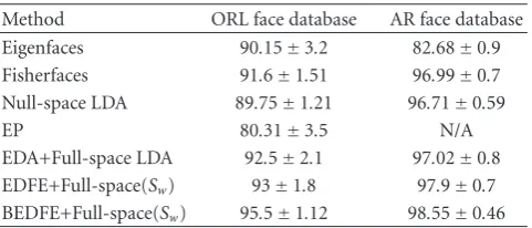
Table4: The mean and standard deviation of recognition accuracy (%) of the proposed EDFE and BEDFE methods and some other state-of-the-art methods on the ORL and AR face databases.

Method ORL face database AR face database Eigenfaces 90.15±3.2 82.68±0.9 Fisherfaces 91.6±1.51 96.99±0.7 Null-space LDA 89.75±1.21 96.71±0.59

EP 80.31±3.5 N/A

EDA+Full-space LDA 92.5±2.1 97.02±0.8 EDFE+Full-space(Sw) 93±1.8 97.9±0.7 BEDFE+Full-space(Sw) 95.5±1.12 98.55±0.46

images for test. For the methods Eigenfaces, Fisherfaces, Null-space LDA, and EP, no validation set is required. Thus we combined the training images and validation images to form the training set for them. The case was a little

bit diﬀerent for the experiments with BEDFE, where the

division of samples is on the class level (each subject is a class). Specifically, we first randomly chose five (seven) images from each subject to compose the test set of the ORL (AR) database. Among the remaining images, a subset of classes was randomly chosen. The samples belonging to these classes were used for training whereas those belonging to the other classes composed the validation set. From each class in the validation set, some samples were randomly chosen to calculate the prototype of the class, and the remaining ones were used for evaluation. On the ORL database, two images of each validation class were randomly chosen for class prototype calculation, and the other three images of the class were used to evaluate the training performance. On the AR database, three images were randomly chosen from each validation class for computing the class prototype, and the other four images of the class were used for training

performance evaluation. The last three columns inTable 1

summarize these settings.

Totally, we created 10 evaluation sets from each of the two databases and ran algorithms over them one by one. We will use the mean and standard deviation of recognition accuracy over the 10 evaluation sets to evaluate the performance of

diﬀerent methods. When applying EP to the ORL databases,

the dimensionality of the data should be reduced in advance due to the high space complexity of EP. We reduced the data to a dimension of the number of training samples minus one

using WPCA (note that the role of WPCA here is diﬀerent

from that in the proposed EDFE algorithm). To evaluate the performance of Eigenfaces on the databases, we tested all possible dimensions of PCA-transformed subspace (between

1 andN−1) and found out the one with the best classification

accuracy. As for Fisherfaces, we set the dimension of

PCA-transformed subspace to the rank ofStand tried all possible

dimensions of LDA-transformed subspace (between 1 and L−1).

4.2. Investigation on Diﬀerent Subspaces. Three subspaces,

null(Sw), range(Sw), and range(Sb), are thought to contain

rich discriminative information within data [16, 17]. As

mentioned above, the algorithms proposed in this paper pro-vide a method to constrain the search in a specific subspace. Hence, we can restrict the algorithms to search for a solution within that subspace. Here we report our experimental results in investigating the above three subspaces using the EDFE and BEDFE algorithms on the ORL and AR databases. Table 2shows the average recognition accuracy of EDFE

in the three diﬀerent subspaces on the ten evaluation sets

of ORL and AR databases. The presented classification accuracies are the best ones among those obtained using

diﬀerent weights. On all the ten evaluation sets of both ORL

and AR databases, null(Sw) gives the best results, which are

significant better than the other two subspaces. On the other

hand, there is no big diﬀerence between the performance

of range(Sw) and range(Sb). This is not surprising because

in the null space ofSw, if exists, samples in the same class

will be condensed to one point. Then if a projection basis

in it can be found to make the samples of diﬀerent classes

separable from each other, the classification performance on these samples will be surely the best. However, for new samples unseen in the training set, the classification accuracy

on them depends on the accuracy of the estimation of Sw.

Another problem with null(Sw) is that its dimensionality is

bounded by the minimum of the dimensionality of the data

and the diﬀerence between the number of samples and the

number of classes. Consequently, as the number of training samples increases, this null space could become too small to

contain suﬃcient discriminant information. In this case, we

propose to incorporate the bagging technique to the EDFE algorithm to enhance its performance. The results of BEDFE

are given inTable 3, from which similar conclusion can be

drawn.

4.3. Investigation on Dimensionality of Feature Subspaces. In order to show the importance of carefully choosing the dimensionality of feature subspaces, we calculated the average recognition accuracy of Eigenfaces and Fisherfaces on the ten evaluation sets taken from the ORL and AR face

databases when diﬀerent numbers of features were chosen for

(9)

0.2 0.1 0.3 0.4 0.5 0.6 0.7 0.8 0.9 1

R

ec

o

gnition r

at

e

0 50 100 150 200

Dimension (number of features)

(a)

0 5 10 15 20 25 30 35 40 0.2

0.1 0 0.3 0.4 0.5 0.6 0.7 0.8 0.9 1

R

ec

o

gnition r

at

e

(b)

160 165 170 175 180 185 190 195 200 0.895

0.896 0.897 0.898 0.899 0.9 0.901 0.902 0.903

R

ec

o

gnition r

at

e

(c)

27 28 29 30 31 32 33 34 35 36 37 0.75

0.8 0.85 0.9 0.95 1

R

ec

o

gnition r

at

e

(d)

Figure4: The curves of the average recognition accuracy of (a) Eigenfaces and (b) Fisherfaces on the ORL face database versus the number of features or the dimension of feature subspaces. (c) and (d) are the corresponding enlarged last parts of the curves.

of LDA-reduced feature subspace from 1 to 119 (i.e., the number of classes minus one). According to the experimental results, the overall trend of recognition accuracy is increasing as the number of features (i.e., the dimension of feature subspace) increases. However, the best accuracy is often obtained not at the largest possible dimension (i.e., the number of samples minus one in case of Eigenfaces and the number of classes minus one in case of Fisherfaces). Figures

4and5show the curves of the average recognition accuracy

of Eigenfaces and Fisherfaces on ORL and AR face databases versus the dimension of feature subspaces (to clearly show that the best accuracy is achieved not necessarily at the largest possible dimension, we also display the last part of the curves in an enlarged view). From these results, we can see that the dimension at which the best recognition accuracy is achieved varies with respect to the datasets. Therefore, using a systematic method like the ones proposed in this paper to automatically determine the dimension of feature subspaces is very helpful to a subspace-based recognition system.

4.4. Performance Comparison. Finally, we compared the proposed algorithms with some state-of-the-art methods in

literature, including Eigenfaces [9], Fisherfaces [10],

Null-space LDA [16], EP [18], and EDA+Full-space LDA [32].

Considering that both null(Sw) and range(Sw) have useful

discriminative information, we ran our proposed EDFE

and BEDFE methods in both null(Sw) and range(Sw) and

then employed the same fusion method used by [32] to

fuse the results obtained in these two subspaces. We called

them EDFE+Full-space(Sw) and BEDFE+Full-space(Sw). We

implemented these methods by using Matlab and evaluated their performance on the ten evaluation sets of ORL and AR face databases. But as for the EP method, it is too computationally complex to be applicable (N/A) on the AR face database (in Matlab an error of ‘out of memory’ will be reported to the EP method). We calculated the mean and standard deviation of the recognition rates for all the

methods. The results are listed in Table 4 (the results of

Eigenfaces and Fisherfaces are according to the best results obtained in the last subsection).

(10)

0 0.1 0.2 0.3 0.4 0.5 0.6 0.7 0.8 0.9

100

0 200 300 400 500 600 700 800 900 Dimension (number of features)

R

ec

o

gnition r

at

e

(a)

0

R

ec

o

gnition r

at

e

0 0.1 0.2 0.3 0.4 0.5 0.6 0.7 0.8 0.9 1

20 40 60 80 100 120

(b)

R

ec

o

gnition r

at

e

680 700 720 740 760 780 800 820 840 0.825

0.8255 0.826 0.8265 0.827 0.8275

(c)

R

ec

o

gnition r

at

e

104 106 108 110 112 114 116 118 120 0.88

0.9 0.92 0.94 0.96 0.98 1

(d)

Figure5: The curves of the average recognition accuracy of (a) Eigenfaces and (b) Fisherfaces on the AR face database versus the number of features or the dimension of feature subspaces. (c) and (d) are the corresponding enlarged last parts of the curves.

systems could be alleviated. Moreover, the improvement on recognition accuracy made by the proposed EDFE and BEDFE compared with the other methods could be due to their better generalization ability. In Eigenfaces, Fisherfaces, Null-space LDA, and EDA+Full-space LDA, the projection basis used for dimension reduction is directly calculated from certain covariance or scatter matrix of the training data. Instead, the methods proposed in this paper begin the search of optimal projection basis from these directly calculated ones and iteratively approach the best one via the linear combination of them. The linear combination not only ensures that the resulting projection basis still lies in the feature subspace but also enhances the generalization ability of the obtained projection basis by adjusting them according to the recognition accuracy on some validation data.

5. Discussion

In the proposed EDFE and BEDFE algorithms, we take the classification accuracy term as a part of the fitness function of the GA. It is then naturally optimized as the GA population evolves. Unlike existing evolutionary computation-based

feature extraction methods like EP [18], we define this term

on a randomly chosen validation sample set, but not the training set. Since the validation set’s role is to simulate

new test samples, the performance of the resulting feature subspace is supposed to be more reliable. We also set up a Fisher criterion-like term as another part of the GA’s fitness function and optimize it in an iterative way, avoiding the matrix inverse operation required by the conventional LDA method. As a result, the proposed algorithms could alleviate the small sample size (SSS) problem of LDA.

Current PCA- and LDA-based subspace methods such as Eigenfaces and Fisherfaces require setting the dimensionality for the feature subspace in advance. They fail to provide sys-tematic way to automatically determine the dimensionality from the classification viewpoint. Since the optimal dimen-sionality of feature subspace in terms of recognition rates will vary across datasets, it is desired to select automatically the optimal dimensionality for specific datasets, instead of using a predefined one. The proposed EDFE and BEDFE algorithms provide such a way by employing the stochastic optimization scheme of GA.

Some other GA-based feature selection/extraction meth-ods have been also proposed in literature. Although these GA-based feature selection methods, such as

EDA+Full-space LDA [32], GA-PCA and GA-Fisher [26], have the

(11)

have high space complexity and are thus not applicable to high dimensional and large scale datasets. For example, in

EP [18], an individual has (5n2₋₄_n_{) bits. In the recently}

proposed EDA algorithm [37], the individual has to encode

(n×m) weights, which are between −0.5 and 0.5 (here,n

is the dimension of the original data space, and m is the

dimension of the feature subspace). On the contrary, the

individual in the proposed algorithms has only (12n−1)

bits (note that in face recognition applications,mis usually

much larger than 12 and a number of bits have to be used to represent a decimal weight used by EDA). As a result, the space complexity is significantly reduced in our proposed methods. After incorporating the bagging technique with the proposed EDFE algorithm, it becomes more stable by

eliminating possible outliers and fusing diﬀerent feature

subspaces, and hence more suitable for high-dimensional and large scale datasets.

Another problem with existing GA-based feature extrac-tion methods lies in their blind search strategy. Using the linear combination and orthogonal complement techniques, the EDFE successfully provides a way to impose constraints on the search space of GA. This also enables EDFE to

eﬀectively make use of the heuristic information of the

dis-criminative feature subspace to improve its search eﬃciency

and classification performance. In addition, the proposed algorithms make it possible to investigate the discriminative

ability of diﬀerent feature subspaces.

6. Conclusions

In this paper, we proposed an evolutionary approach to extracting discriminative features, namely, evolutionary dis-criminant feature extraction (EDFE) as well as its bagging version (BEDFE). The basic idea underlying the EDFE algorithm is to use the genetic algorithm (GA) to search for an optimal discriminative projection basis in a constrained

subspace with the goal of making the data in diﬀerent clusters

much easier to be separated. The primary contribution of this paper includes (1) reducing the space complexity of GA-based feature extraction algorithms; (2) enhancing the

search eﬃciency, stability, as well as recognition accuracy;

(3) providing an eﬀective way to investigate diﬀerent feature

subspaces. Experiments on the ORL and AR databases have been performed to validate the proposed methods.

There are still some issues worthy further study on the proposed approach. Firstly, it is a supervised linear feature extraction method. Therefore, how to extend it to nonlinear cases deserves further study. Secondly, the latest progress in the research on GA, for example, how to set up an initial population and how to choose proper GA parameters, could give us some useful hints on further improving the proposed methods. Thirdly, more promising results could be obtained by exploring other criteria to evaluate the feature subspaces and incorporating them into the evolutionary approach, for instance, those of recently proposed manifold learning

algorithms [40,41]. Finally, it could be very interesting to

investigate the discriminability of other subspaces using the proposed EDFE and BEDFE algorithms.

Appendix

Proof of

Theorem 1

Proof. First it can be easily proved that for all i ∈

{1, 2,. . .,m−1},βi ∈ A. Sinceβi = Pβi =

m

j=1βi jαj,βi

can be represented by a basis ofA. Thusβi∈A.

Secondly, let us proveA=U⊕V, whereU =span{β1,

β2,. . .,βm−1}. This is to prove that{β1,β2,. . .,βm−1,v}is a

linear independent bundle. Sinceβi =PβiandPTP =Em,

which is anm-dimensional identity matrix, we haveβT

iβj =

βT

iβj. However, {βi | i = 1, 2,. . .,m−1} is an identity

orthogonal basis. Thus, β1,β2,. . .,βm−1 are orthogonal to

each other.

Furthermore, for all i ∈ {1, 2,. . .,m − 1}, βT

iv =

(Pβi)Tv = βTiPTv. Because {βi | i = 1, 2,. . .,m−1} is

an identity orthogonal basis of the orthogonal complement

space ofV = span{PT_v_} _in_Rm_, _βT

i(PTv) should be zero.

Therefore,βTiv=0, that is,βiis also orthogonal tov.

To sum up, we get that {β1,β2,. . .,βm−1,v} is a linear

independent bundle containingmorthogonal vectors in the

mdimensional spaceA. ThusA=U⊕V.

Acknowledgment

This work is partially supported by the Hong Kong RGC General Research Fund (PolyU 5351/08E).

References

[1] D. Zhang and X. Y. Jing, Biometric Image Discrimination Technologies, Idea Group, 2006.

[2] P. J. Phillips, P. J. Flynn, T. Scruggs, et al., “Overview of the face recognition grand challenge,” inProceedings of the IEEE Computer Society Conference on Computer Vision and Pattern Recognition (CVPR ’05), vol. 1, pp. 947–954, June 2005. [3] W. Zhao, R. Chellappa, P. J. Phillips, and A. Rosenfeld, “Face

recognition: a literature survey,”ACM Computing Surveys, vol. 35, no. 4, pp. 399–458, 2003.

[4] N. V. Chawla and K. W. Bowyer, “Actively exploring creation of face space(s) for improved face recognition,” inProceedings of the 22nd National Conference on Artificial Intelligence (AAAI ’07), vol. 1, pp. 809–814, Vancouver, Canada, July 2007. [5] K. Fukunaga, Introduction to Statistical Pattern Recognition,

Academic Press, San Diego, Calif, USA, 2nd edition, 1990. [6] N. A. Schmid and J. A. O’Sullivan, “Thresholding method

for dimensionality reduction in recognition systems,” IEEE Transactions on Information Theory, vol. 47, no. 7, pp. 2903– 2920, 2001.

[7] I. T. Jolliﬀe,Principal Component Analysis, Springer, New York, NY, USA, 2nd edition, 2002.

[8] E. Oja,Subspace Methods of Pattern Recognition, John Wiley & Sons, New York, NY, USA, 1983.

[9] M. Turk and A. Pentland, “Eigenfaces for recognition,”Journal of Cognitive Neuroscience, vol. 13, no. 1, pp. 71–86, 1991. [10] P. N. Belhumeur, J. P. Hespanha, and D. J. Kriegman,

(12)

[11] K. Messer, J. Kittler, M. Sadeghi, et al., “Face authentication test on the BANCA database,” in Proceedings of the 17th International Conference on Pattern Recognition, vol. 3, pp. 523–532, 2004.

[12] B. Moghaddam, A. Pentland, et al., “Probabilistic visual learning for object representation,” IEEE Transactions on Pattern Analysis and Machine Intelligence, vol. 19, no. 7, pp. 696–710, 1997.

[13] B. Moghaddam, T. Jebara, A. Pentland, et al., “Bayesian face recognition,”Pattern Recognition, vol. 33, no. 11, pp. 1771– 1782, 2000.

[14] X. Wang and X. Tang, “A unified framework for subspace face recognition,”IEEE Transactions on Pattern Analysis and Machine Intelligence, vol. 26, no. 9, pp. 1222–1228, 2004. [15] M. Kirby and L. Sirovich, “Application of the Karhunen-Loeve

procedure for the characterization of human faces,” IEEE Transactions on Pattern Analysis and Machine Intelligence, vol. 12, no. 1, pp. 103–108, 1990.

[16] L.-F. Chen, H.-Y. M. Liao, M.-T. Ko, J.-C. Lin, and G.-J. Yu, “New LDA-based face recognition system which can solve the small sample size problem,”Pattern Recognition, vol. 33, no. 10, pp. 1713–1726, 2000.

[17] J. Yang, A. F. Frangi, J.-Y. Yang, D. Zhang, and Z. Jin, “KPCA plus LDA: a complete kernel fisher discriminant framework for feature extraction and recognition,”IEEE Transactions on Pattern Analysis and Machine Intelligence, vol. 27, no. 2, pp. 230–244, 2005.

[18] C. J. Liu and H. Wechsler, “Evolutionary pursuit and its application to face recognition,”IEEE Transactions on Pattern Analysis and Machine Intelligence, vol. 22, no. 6, pp. 570–582, 2000.

[19] W. Siedlecki and J. Sklansky, “A note on genetic algorithms for large-scale feature selection,”Pattern Recognition Letters, vol. 10, no. 5, pp. 335–347, 1989.

[20] H. Vafaie and K. De Jong, “Genetic algorithms as a tool for restructuring feature space representations,” in Proceedings of the 7th International Conference on Tools with Artificial Intelligence, pp. 8–11, 1995.

[21] H. Vafaie and K. De Jong, “Feature space transformation using genetic algorithms,”IEEE Intelligent Systems and Their Applications, vol. 13, no. 2, pp. 57–65, 1998.

[22] M. G. Smith and L. Bull, “Feature construction and selec-tion using genetic programming and a genetic algorithm,” in Proceedings of the 6th European Conference on Genetic Programming (EuroGP ’03), C. Ryan, et al., Ed., vol. 2610 ofLecture Notes in Computer Science, pp. 229–237, Springer, Berlin, Germany, August 2003.

[23] M. Pei, et al., “Genetic algorithms for classification and feature extraction,” inProceedings of the Annual Meeting of the Classification Society of North America (CSNA ’95), pp. 22–25, Denver, Colo, USA, June 1995.

[24] M. L. Raymer, W. F. Punch, E. D. Goodman, L. A. Kuhn, and A. K. Jain, “Dimensionality reduction using genetic algorithms,”

IEEE Transactions on Evolutionary Computation, vol. 4, no. 2, pp. 164–171, 2000.

[25] Q. Zhao and H. Lu, “GA-driven LDA in KPCA space for facial expression recognition,” inProceedings of the 1st International Conference on Natural Computation (ICNC ’05), vol. 3611 of Lecture Notes in Computer Science, pp. 28–36, Springer, Changsha, China, August 2005.

[26] W.-S. Zheng, J.-H. Lai, and P. C. Yuen, “GA-Fisher: a new LDA-based face recognition algorithm with selection of principal components,”IEEE Transactions on Systems, Man, and Cybernetics, Part B, vol. 35, no. 5, pp. 1065–1078, 2005.

[27] Q. Zhao, H. Lu, and D. Zhang, “A fast evolutionary pursuit algorithm based on linearly combining vectors,” Pattern Recognition, vol. 39, no. 2, pp. 310–312, 2006.

[28] D. Dumitrescu,Evolutionary Computation, CRC Press, 2000. [29] Q. Zhao, D. Zhang, and H. Lu, “A direct evolutionary feature

extraction algorithm for classifying high dimensional data,” in

Proceedings of the National Conference on Artificial Intelligence (AAAI ’06), vol. 1, pp. 561–566, Boston, Mass, USA, 2006. [30] D. Goldberg,Genetic Algorithm in Search, Optimization, and

Machine Learning, Adison-Wesley, 1989.

[31] Q. Zhao, H. Lu, and D. Zhang, “Parsimonious feature extraction based on genetic algorithms and support vector machines,” inLecture Notes in Computer Science, vol. 3971, pp. 1387–1393, Springer, Berlin, Germany, May 2006.

[32] X. Li, B. Li, H. Chen, X. Wang, and Z. Zhuang, “Full-space LDA with evolutionary selection for face recognition,” in

Proceedings of the International Conference on Computational Intelligence and Security (ICCIAS ’06), vol. 1, pp. 696–701, November 2006.

[33] X. Wang and X. Tang, “Random sampling for subspace face recognition,”International Journal of Computer Vision, vol. 70, no. 1, pp. 91–104, 2006.

[34] L. Breiman, “Bagging predictors,”Machine Learning, vol. 24, no. 2, pp. 123–140, 1996.

[35] J. Kittler, M. Hatef, R. P. W. Duin, and J. Matas, “On combining classifiers,”IEEE Transactions on Pattern Analysis and Machine Intelligence, vol. 20, no. 3, pp. 226–239, 1998.

[36] J. Kittler and F. M. Alkoot, “Sum versus vote fusion in multiple classifier systems,”IEEE Transactions on Pattern Analysis and Machine Intelligence, vol. 25, no. 1, pp. 110–115, 2003. [37] A. Sierra and A. Echeverria, “Evolutionary discriminant

analysis,”IEEE Transactions on Evolutionary Computation, vol. 10, no. 1, pp. 81–92, 2006.

[38] F. S. Samaria and A. C. Harter, “Parameterisation of a stochastic model for human face identification,” inProceedings of the 2nd IEEE Workshop on Applications of Computer Vision, pp. 138–142, 1994.

[39] A. M. Martinez and R. Benavente, “The AR face database,” Tech. Rep. 24, 1998.

[40] S. T. Roweis and L. K. Saul, “Nonlinear dimensionality reduction by locally linear embedding,”Science, vol. 290, no. 5500, pp. 2323–2326, 2000.