Descriptive Statistics (PART I)

Introductory Statistics

ECON1005

I

I

Descriptive Statistics (PART

_{Descriptive Statistics (PART}

I)

I)



Introduction

INTRODUCTION

INTRODUCTION



_{What is Statistics?}



_{Basic Definitions}



_{Summarising & Describing}

What is Statistics?

•

Statistics

is a group of methods

used to collect, analyse, display and

interpret data and to make

Branches of Statistics

STATISTICS

DESCRIPTIVE STATISTICS (characterise attributes of sample

&/or population)

INFERENTIAL STATISTICS (make generalisations about

•

Used to collect, organize, display and analyse

data

•

There are two types:

1. Numerical

 _{Involves the computation of a statistic (eg. the}

average)

2. Graphical

 _{Involves representing the data using pictures}

 _Eg.

Summary of Statistics Grades

A 42%

B+ 13% B

2% C

Inferential Statistics

•

Uses sample results to make generalizations,

inferences and predictions about a wider

population

•

There are two types:

▫ Estimation

 _{sample is used to estimate a parameter}

▫ Hypothesis Testing

 _{a "hypothesis” is put forward and it is determined}

Descriptive vs. Inferential Statistics

•

Descriptive

_Descriptive

Statistics

Statistics

▫ Collect

▫ Organize

▫ Summarize

▫ Display

▫ Analyze

•

Inferential Statistics

_{Inferential Statistics}

▫ Predict and forecast

values of a population

▫ Test hypotheses about

values of a population

Basic Definitions I

•

Population

:

▫ A population is the collection of all items whose characteristics are being studied.

 _{N represents the population size}

▫ Values calculated using population data are called

parameters

•

Sample:

_Sample

▫ A sample is a portion of the population selected for study.

 _{n represents the sample size}

Basic Definitions II

•

Data:

_Data

▫ numbers or measurements that are collected

•

Variables:

_Variables

▫ characteristics or attributes that enable us to distinguish one individual from another

▫ they take on different values when different individuals are observed (e.g. height)

•

Element:

_Element

Summarising & Describing Data

•

Describing the observed patterns in data

is an important part of statistics

•

Distribution of a single variable

Describing Data

S

Shape

U

Unusual

M

Middle

Organizing and Graphing Data

Organizing and Graphing Data



_Introduction



_{Frequency Distributions}



_{Bar Charts}

Introduction

• There are two main types of data:

▫ Quantitative

 _{This is information presented in the form of numbers,}

percentages or statistics

 It answers in numerical terms such questions as "how often" and "how many“

▫ Qualitative

 Records a thought, observation, opinion, or words

A frequency distribution lists all

Frequency Distributions

▫ a table in which measurements are tallied

▫ then the frequency or total number of times that each item occurs is recorded

• Usually measurements are arranged in ascending or descending order

• A frequency distribution has 3 columns

▫ the data categories or classes

▫ the tally column (for raw data) ▫ the corresponding frequencies

Examples

•

Quantitative

•

Qualitative

CATEGORY TALLY FREQUENCY

Yes 23

No 13

Undecided 4

Total 40

10M - 14M 25

15M - 19M 15

20M - 24M 19

25M - 29M 8

Total 77

Frequency Distribution Cont’d

•

two main types of frequency distributions:

▫Ungrouped data

▫Grouped data

5M - 9M 10

10M - 14M 25

15M - 19M 15

20M - 24M 19

25M - 29M 8

Total 77

Ages Tally Frequency

•

Class Intervals/Limits

_{Class Intervals/Limits}

▫largest or smallest numbers which can

actually belong to each class

▫each class has a

lower class limit

and an

upper class limit

expenditure (J$M)

Tally Number of Firms

5 - 9 10

10 – 14 25

15 – 19 15

20 – 24 19

25 - 29 8

Total 77

Class Limits

Lower Class Limit

▫ the numbers which separate classes

▫ given by the midpoint of the upper limit of one

class and the lower limit of the next class

Ad. expenditure (J$M) Class Boundaries Tally Number of Firms

5 - 9 10

10 – 14 9.5 – 14.5 25

15 – 19 15

20 – 24 19

25 - 29 8

Total 77

Lower class boundary for 2nd class

(10 – 14):

2 2 class for limit class lower 1 class for limit class

upper 

5 . 9 2 10 9  

Upper class boundary for 2nd class (10 – 14):

2 3 class for limit class lower 2 class for limit class

upper 

•

Class Mark (Midpoint)

_{Class Mark (Midpoint)}

▫ found by taking the average of the class limits (or

class boundaries)

5 - 9 4.5 – 9.5 7 10

10 – 14 9.5 – 14.5 25

15 – 19 14.5 – 19.5 15

20 – 24 19.5 – 24.5 19

25 - 29 24.5 – 29.5 8

Total 77

Class 1 - Using Class Limits

2 1 class for limit class upper 1 class for limit class

lower 

7 2 9 5  

Class 1 - Using Class Boundaries

2 1 class for boundary class upper 1 class for boundary class

lower 

•

Class Width

_{Class Width}

▫ aka: class size, class width, class length ▫ Two ways of calculating

▫ Method 1: the difference between corresponding class limits

▫ Method 2: the difference between two class boundaries

Ad. expenditure (J$M) Class Boundaries Midpoints Number of Firms

5 - 9 4.5 – 9.5 7 10

10 – 14 9.5 – 14.5 12 25

15 – 19 14.5 – 19.5 17 15

20 – 24 19.5 – 24.5 22 19

25 - 29 24.5 – 29.5 27 8

Total 77

Using Class Limits

1 limit class lower -2 limit class lower 5 5

10  

Using Class Boundaries

1 boundary class lower -1 boundary class upper 5 5 . 4 5 .

•

Found by dividing the frequency of a

category/class by the sum of all frequencies

▫ The sum of the relative frequencies MUST add to 1

▫ Sometimes expressed as a percentage

Ad. expenditure (J$M) Class Boundaries Number of Firms Relative Frequency

5 - 9 4.5 – 9.5 10 0.13

10 – 14 9.5 – 14.5 25

15 – 19 14.5 – 19.5 15

20 – 24 19.5 – 24.5 19

25 - 29 24.5 – 29.5 8

Total 77 1.00

General Formula Total Frequency Frequency Relative  Class 1 13 . 0 77 10 Total Frequency Frequency

Distributions

1. The classes must be “mutually exclusive” - no element can belong to more than one class

2. Even if the frequency is zero, include each and every class

3. Make all classes the same width (open ended classes may be inevitable)

4. Target between 5 and 20 classes, depending on the range and number of data points

Consider the following data set:

2.3 4.2 2.8 6.7 4.7 1.6 2.0 1.4 1.0

2.8 1.8 5.2 6.0 5.2 3.5 1.0 3.6 5.1

1.9 7.3 2.5 5.6 3.3 3.4 2.9 3.0 1.8

2.1 3.1 2.8 2.1 4.3 7.1 4.9 1.6 2.2

4.5 6.3 2.7 8.3

a. Group these figures into a frequency distribution having

the classes: 1.0 – 1.9, 2.0 – 2.9, 3.0 – 3.9, 4.0 – 4.9, 5.0 – 5.9, 6.0 – 6.9, 7.0 – 7.9, and 8.0 – 8.9

b. Calculate the class boundaries

c. Calculate the class midpoints

d. Calculate the class width

Graphical Representation

•

When presenting

Quantitative Data

use:

▫histograms

▫frequency polygons

▫cumulative frequency polygons (O-give)

•

When presenting

Qualitative Data

use:

▫ A graphical way of presenting

qualitative data

•

Bars (columns) are separated from each other

and have the same width

•

Categories are placed on the horizontal axis and

frequencies (or relative frequencies)on the

▫ A graphical way of presenting

qualitative data

•

Pie Chart is a circle divided into portions that

represent the relative frequencies belonging to

different categories.

•

To construct pie chart:

Qualitative Example

The following are the results for a third year

statistics course:

A - 41

B+ - 12

B - 2

C - 22

F - 19

▫ Calculate the relative frequencies

▫ Construct a bar chart

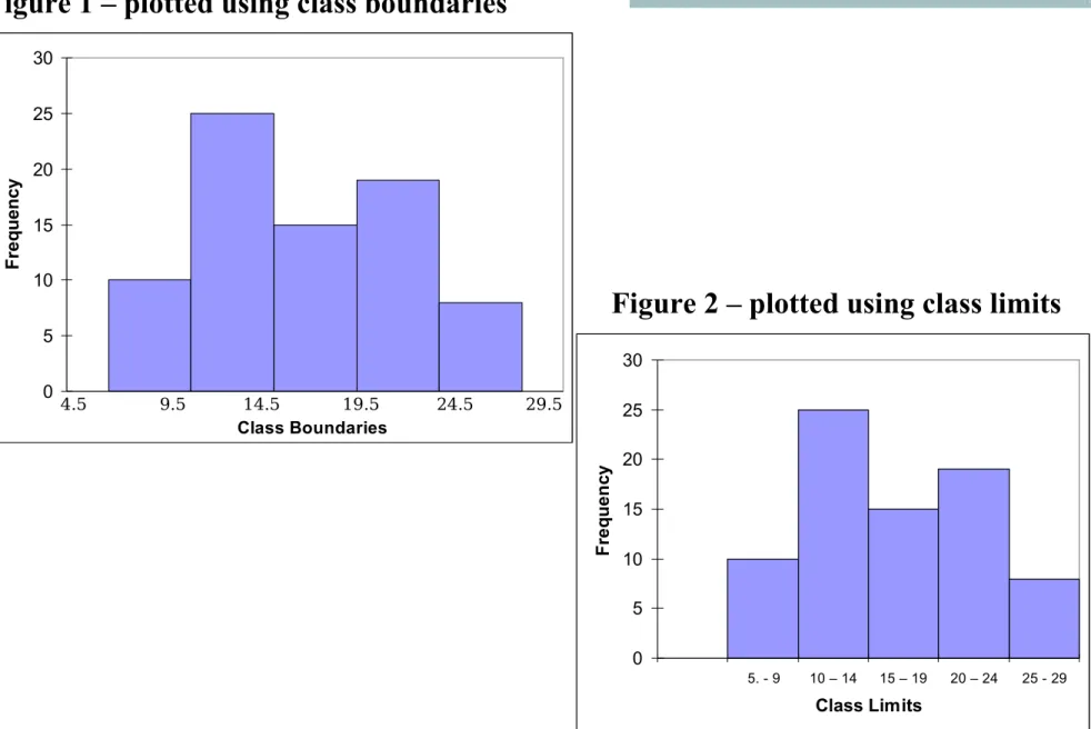
• A graphical way of presenting qualitative data

• Divide data into classes of equal width and the number of

observations in each class is counted (information would be presented in a frequency table)

• Class is on the x-axis (horizontal)

▫ Can plot using either:

 Class Limits

 Class Boundaries

• Frequency (or relative frequency) is on the y-axis (vertical)

• Bars are drawn where the base of each bar covers the

class and the height of each bar covers the frequency

Figure 2 – plotted using class limits 0 5 10 15 20 25 30

5. - 9 10 – 14 15 – 19 20 – 24 25 - 29

Class Limits F re q u en cy 0 5 10 15 20 Class Boundaries F re q u en cy

4. Frequency Polygons

•

A

Frequency Polygon

is a line graph joining

the midpoints of the bars of a histogram

•

To construct a frequency polygon:

▫ Plot the midpoint of each class (on horizontal) with

its corresponding frequency/relative frequency (on

vertical)

0 5 10 15 20 25

5. - 9 10 – 14 15 – 19 20 – 24 25 - 29

Class Limits

F

re

q

u

en

cy

• _{Examines how many observations} lie below a certain class boundary

• Plotted against the upper class boundaries

Using Frequencies

• The first value in the distribution is ALWAYS zero

• The last value in the distribution is ALWAYS the total

number

Using Relative Frequencies

• The first value in the distribution is ALWAYS zero

• The last value in the distribution is ALWAYS 1

Using Percentages

• The first value in the distribution is ALWAYS zero

0 10 20 30 40 50 60 70 80 90

4.5 9.5 14.5 19.5 24.5 29.5

Class Boundaries F re q u en c y expenditure (J$M) Upper Class Boundaries Number

of Firms Cumulative _Frequency

4.5

5 - 9 9.5 10

10 – 14 14.5 25

15 – 19 19.5 15

20 – 24 24.5 19

25 - 29 29.5 8

-• Examines how many observations lie above a certain class boundary

• Plotted against the upper class boundaries

Using Frequencies

• The first value in the distribution is ALWAYS the total

number

• The last value in the distribution is ALWAYS zero

Using Relative Frequencies

• The first value in the distribution is ALWAYS 1

• The last value in the distribution is ALWAYS zero

Using Percentages

• The first value in the distribution is ALWAYS 100

Ad. expenditure (J$M) Upper Class Boundaries Number of Firms More Than Cumulative Frequency 4.5

5 - 9 9.5 10

10 – 14 14.5 25

15 – 19 19.5 15

20 – 24 24.5 19

25 - 29 29.5 8

Total - 77

-0 10 20 30 40 50 60 70 80 90

4.5 9.5 14.5 19.5 24.5 29.5

•

Using the example on

slide 25

,

a. Construct a histogram with a

superimposed frequency polygon

b. Calculate:



_{Less than cumulative frequencies}



_{More than cumulative frequencies}

c. Construct the: