Thesis by
Kevin Qing Shan
In Partial Fulfillment of the Requirements for the Degree of
Doctor of Philosophy
CALIFORNIA INSTITUTE OF TECHNOLOGY Pasadena, California
2019
ii
© 2019
Kevin Qing Shan
ORCID: 0000-0002-2621-1274
ACKNOWLEDGEMENTS
First, I would like to thank Thanos Siapas for his support and mentorship over all
these years, and the rest of my committee—Joel Burdick, Richard Murray, and
Michael Dickinson—for everything they’ve done to make this thesis happen.
Thanks also to Eugene Lubenov for invaluable discussions and feedback (including
on this document), to Andreas Hoenselaar for being a positive role model for
software development practices, to Britton Sauerbrei for his dedication to data
visualization, and to Brad Hulse and Maria Papadopoulou for their conversations
and commiserations, both intellectual and otherwise.
I’d also like to thank my CDS cohort—Seungil, Ivan, Anandh—and other Caltech
friends—Andrew, Hannah, Denise, Max, Ioana—for being part of my life outside the lab. Finally, I am immensely grateful to my parents and my brother Kyle for
their constant support and encouragment, and to my wonderful wife Sze for all of the
iv
ABSTRACT
Chronic extracellular recording is the use of implanted electrodes to measure the
electrical activity of nearby neurons over a long period of time. It presents an
unparalleled view of neural activity over a broad range of time scales, offering
sub-millisecond resolution of single action potentials while also allowing for continuous recording over the course of many months. These recordings pick up a rich collection
of neural phenomena—spikes, ripples, and theta oscillations, to name a few—that
can elucidate the activity of individual neurons and local circuits.
However, this also presents an interesting challenge for data analysis. Chronic
extracellular recordings contain overlapping signals from multiple sources, requiring
these signals to be detected and classified before they can be properly analyzed. The
combination of fine temporal resolution with long recording durations produces large datasets, requiring efficient algorithms that can operate at scale.
In this thesis, I consider the problem of spike sorting: detecting spikes (the
extracellu-lar signatures of individual neurons’ action potentials) and clustering them according
to their putative source. First, I introduce a sparse deconvolution approach to spike
detection, which seeks to detect spikes and represent them as the linear combination
of basis waveforms. This approach is able to separate overlapping spikes without the
need for source templates, and produces an output that can be used with a variety of
clustering algorithms.
Second, I introduce a clustering algorithm based around a mixture of drifting
t-distributions. This model captures two features of chronic extracellular recordings— cluster drift over time and heavy-tailed residuals in the distribution of spikes—that
are missing from previous models. This enables us to reliably track individual
neurons over longer periods of time. I will also show that this model produces more
accurate estimates of classification error, which is an important component to proper
interpretation of the spike sorting output.
Finally, I present a few theoretical results that may assist in the efficient implementation
PUBLISHED CONTENT AND CONTRIBUTIONS
Shan, K. Q., E. V. Lubenov, and A. G. Siapas (2017). “Model-based spike sorting with a mixture of drifting t-distributions”.Journal of neuroscience methods288, pp. 82–98. doi:10.1016/j.jneumeth.2017.06.017.
KQS conceived of the project, developed and analyzed the method, collected some of the validation data, and wrote the manuscript.
Shan, K. Q., E. V. Lubenov, M. Papadopoulou, and A. G. Siapas (2016). “Spatial tuning and brain state account for dorsal hippocampal CA1 activity in a non-spatial learning task”.Elife5, e14321. doi:10.7554/eLife.14321.001.
vi
TABLE OF CONTENTS
Acknowledgements . . . iii
Abstract . . . iv
Published Content and Contributions . . . v
Table of Contents . . . vi
List of Illustrations . . . vii
Chapter I: Introduction . . . 1
Chapter II: Spike detection via sparse deconvolution . . . 5
2.1 Introduction . . . 5
2.2 Methods . . . 8
2.3 Results . . . 17
2.4 Discussion . . . 19
Chapter III: Spike sorting using a mixture of driftingt-distributions . . . 20
3.1 Introduction . . . 20
3.2 Mixture of driftingt-distributions (MoDT) model . . . 23
3.3 Model validation using empirical data . . . 32
3.4 Use of the MoDT model for measuring unit isolation . . . 39
3.5 Overlapping spikes . . . 46
Chapter IV: Improving regularizers for sparse deconvolution . . . 49
4.1 The nonconvex log regularizer . . . 50
4.2 Nested group regularizers . . . 59
Chapter V: Conclusion . . . 72
LIST OF ILLUSTRATIONS
Number Page
1.1 An overview of spike sorting . . . 2
2.1 Spike detection as a sparse deconvolution problem . . . 6
2.2 Issues with the convexl2,1regularizer . . . 13
2.3 Comparison of optimization algorithms . . . 15
2.4 Spike detection performance on a hybrid ground truth dataset . . . . 17
2.5 Spike removal for LFP analysis . . . 18
3.1 Extracellular recordings contain drifting, heavy-tailed clusters . . . . 21
3.2 Scaling of computational runtime with MoDT model dimensions . . 28
3.3 Robust covariance estimation using thet-distribution . . . 30
3.4 Cluster drift in well-isolated units . . . 33
3.5 Heavy-tailed residuals in extracellular noise and well-isolated units . 34 3.6 Failure modes of a stationary approach . . . 36
3.7 Spike sorting performance . . . 43
3.8 Comparison of unit quality metrics on hybrid ground truth datasets . 43 3.9 Spike sorting performance on overlapping spikes . . . 46
3.10 Model-based overlap reassignment . . . 47
4.1 Application of the nonconvex log regularizer to a sparse deconvolution problem . . . 50
4.2 An illustration of the proximal operator of the log regularizer . . . . 53
4.3 Comparison of the proximal operator to prior work . . . 58
1
C h a p t e r 1
INTRODUCTION
Chronic extracellular recordings are a powerful tool for systems neuroscience,
offering access to the spiking activity of neurons over long periods over time. In
this technique, recording electrodes are chronically implanted in the brain to monitor
the activity of nearby neurons. Unlike imaging techniques, these passive recordings
do not damage the tissue through photobleaching or require expression of foreign
fluorophores, enabling continuous recordings over the course of many weeks or even months. The ability to continuously monitor individual neurons over these time
scales is critical to advancing our understanding of learning and memory.
However, the analysis of extracellular data requires a process known as spike sorting,
in which spikes—the extracellular signatures of individual neurons’ action potentials—
are detected in the raw data and then assigned to putative sources (i.e., individual
neurons, also known as single units). This process is summarized in Figure 1.1 and
is typically broken into two stages: (1)spike detection, in which spikes are detected as discrete events in a noisy signal, and (2) clustering, an unsupervised learning problem in which the detected spikes are assigned to putative sources.
Unfortunately, prior work on this topic have two important shortcomings that prevent
us from achieving our goal of continuous monitoring of spiking activity over long time
scales. In this document, I develop new methods to overcome these shortcomings.
First, traditional spike detection methods do not account for overlapping spikes, i.e.,
spikes from different neurons that occur nearly synchronously and thus overlap in time. This is a rare occurrence, since the duration of individual spikes is short relative
to the average time between spikes, so traditional techniques can achieve a reasonable
overall performance despite failing to account for this overlap. However, the brain
sometimes exhibits patterns of coordinated activity that increase the prevalence of
overlapping spikes, and these patterns are of special interest to researchers. For
example, during a hippocampal activity pattern known as aripple, a sizeable fraction of pyramidal neurons all fire in close succession. These population bursts are a
prominent feature of slow-wave sleep (Siapas and Wilson, 1998), appear to be
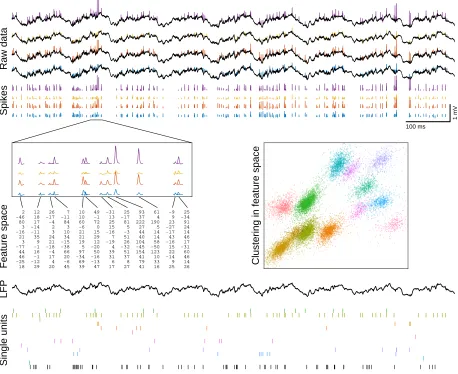
100 ms 1 mV Raw data Spikes 18 -25 46 44 -77 3 21 -16 3 80 -46 2 29 -12 -1 16 -1 9 35 -11 -14 17 18 12 20 4 17 -4 -18 21 24 3 2 -4 -17 26 45 -6 20 66 -38 -15 34 10 3 84 -11 7 39 69 -34 97 5 19 21 21 -6 60 10 10 47 -13 -16 50 -20 12 29 15 0 72 -1 49 17 6 31 39 4 -19 7 -16 15 25 13 -31 27 8 37 51 -32 26 51 -3 5 81 -17 25 41 79 41 154 -45 104 40 44 27 222 37 93 16 33 10 123 -50 58 14 14 5 190 4 61 25 9 -14 22 15 -16 43 -17 -27 23 9 -9 26 14 46 60 -31 17 46 14 24 91 -34 25
Feature space Clustering in feature space
LFP
Single units
Figure 1.1: An overview of spike sorting. Spike sorting is the process of detecting spikes
(the extracellular signatures of neuronal action potentials) and assigning them to putative sources. Raw data:Voltage traces from the four channels of a tetrode (a four-site recording
probe constructed from bundled microwires) in hippocampal area CA1 of a freely-behaving rat. Spikes: During spike detection, we detect spikes in the raw data and extract their
waveforms for downstream analysis. The shape of the spike waveforms (particularly the relative amplitude across the different channels) can be used to classify individual spikes as originating from different sources. Feature space: This information about each spike’s
waveform is represented as a point in some low-dimensional feature space (the 12-dimensional column vectors in this illustration), a format that is amenable to analysis with a variety of unsupervised clustering algorithms. Clustering in feature space: This step groups the
spikes into clusters and produces an estimate of the misclassification error. Single units:
Well-isolated clusters that satisfy the appropriate criteria are known as single units and may be interpreted as the spiking activity of individual neurons (shown as a raster plot here). The last row (black) shows the detected spikes that were not classified as belonging to a single unit. LFP:After spikes have been detected and removed from the raw data, the residual
3
Improving spike detection during these synchronous bursts is thus an important step
to advancing our understanding of these phenomena.
To this end, Chapter 2 describes a sparse deconvolution approach to spike detection.
This procedure approximates the observed signal as the convolution of a set of kernels
(representing the linear subspace of typical spike waveforms) with a column-sparse
feature matrix (which are the detected spikes). This approach explicitly accounts for
overlapping spikes and is able to reliably separate the contribution from each spike.
Unlike the class of techniques known astemplate matching, this approach does not require fitting a source template for each neuron and does not seek to assign the
detected spikes to putative sources. It instead represents the detected spikes as points in a low-dimensional feature space, a format that is amenable to downstream analysis
using a wide variety of clustering algorithms. This approach thereby maintains the
traditional decoupling of spike detection from the clustering problem.
The second shortcoming of prior spike-sorting methods lies in the clustering of long
datasets. Traditional clustering algorithms have been fairly successful when applied to
recordings up to an hour, which is the duration of a typical behavioral training session.
However, many behavioral tasks require multiple days to learn (Shan et al., 2016),
and the process of memory consolidation—the transfer of long-term memories from
the hippocampus to cortical brain areas—may require weeks (Takehara, Kawahara, and Kirino, 2003). The ability to observe changes in neural activity over these
time scales is therefore critical to understanding the neural mechanisms underlying
learning and memory. Although there are few experimental barriers to acquiring
such long-term, continuous recordings, the analysis of such datasets presents a
major challenge to traditional clustering algorithms. This is because the clusters
corresponding to individual neurons drift substantially on the time scale of hours
(due to a combination of electrode motion and physiological changes in the neurons),
which violates the traditional assumption of cluster stationarity.
To address this issue, Chapter 3 describes a clustering algorithm based around fitting the data with a mixture of driftingt-distributions. This generative model captures two important features of chronic extracellular recordings—cluster drift over time
and heavy tails in the distribution of spikes—that are missing from previous models.
This model also provides accurate estimates of classification error, an important
metric for proper interpretation of the spike sorting output.
Finally, Chapter 4 derives some mathematical results (proximal operators for the
5
C h a p t e r 2
SPIKE DETECTION VIA SPARSE DECONVOLUTION
2.1 Introduction
The first step in spike sorting is detecting the spikes to be sorted. The earliest
methods for spike detection simply involved bandpass filtering the signal and
detecting threshold-crossings. Refinements to this technique include the use of data
transformations such as the nonlinear energy operator (Mukhopadhyay and Ray, 1998) or a wavelet transform (Yang and Shamma, 1988; Nenadic and Burdick, 2005)
prior to thresholding. These transformations seek to improve detection performance
by accentuating certain features of neural spikes that distinguish them from the
background noise. After spikes are detected, their waveforms—a short segment of
data centered around each detected spike—may be extracted and then projected into
a low-dimensional feature space for subsequent clustering.
While this approach works well for isolated spikes, it can fail to detect spikes that
occur in close succession (less than 1 ms apart), since the overlapping waveforms may
fail to trigger the detection. Even if both spikes are detected, the presence of the other
spike may distort the observed waveform, leading to downstream misclassification
error if the contribution of the other spike is not accounted for1.
The issue of overlapping spikes is greatest in areas with a high density of cells, such
as the hippocampal pyramidal cell layer, since this leads to a large number of neurons within the electrode’s recording volume. This is further compounded by synchronous
activity patterns, such as ripples, that may cause a large number of neurons to fire
within a short window of time.
An alternative class of spike detection methods, known as template matching,
addresses this issue by seeking to approximate the observed data as the sum of
template waveforms (Bankman, Johnson, and Schneider, 1993; Pachitariu et al.,
2016; Yger et al., 2018), which may be understood as a form of sparse deconvolution
(Figure 2.1A). Each template corresponds to a different source, so detecting a spike
and assigning it to a putative neuron occur as a single step. Although finding the
1I had previously developed a method to do precisely this (Shan, Lubenov, and Siapas, 2017,
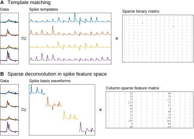
Data
B Sparse deconvolution in spike feature space
Spike basis waveforms
15 22 13 116 -44 40 19 12 11 185 8 48 46 19 -11 72 37 -4 68 15 -30 143 86 -59 0 0 0 0 0 0 0 0 0 0 0 0 0 0 0 0 0 0 0 0 0 0 0 0 0 0 0 0 0 0 0 0 0 0 0 0 0 0 0 0 0 0 0 0 0 0 0 0 0 0 0 0 0 0 0 0 0 0 0 0 0 0 0 0 0 0 0 0 0 0 0 0 0 0 0 0 0 0 0 0 0 0 0 0 0 0 0 0 0 0 0 0 0 0 0 0 0 0 0 0 0 0 0 0 0 0 0 0 0 0 0 0 0 0 0 0 0 0 0 0 0 0 0 0 0 0 0 0 0 0 0 0 0 0 0 0 0 0 0 0 0 0 0 0 0 0 0 0 0 0 0 0 0 0 0 0 0 0 0 0 0 0 0 0 0 0 0 0 Column-sparse feature matrix
Data
A Template matching
Spike templates 0 0 0 0 0 0 0 0 0 0 0 0 0 0 1 0 0 0 0 0 0 0 0 0 0 0 0 0 0 1 0 0 0 0 0 0 0 0 0 0 0 0 0 0 0 0 0 0 0 0 0 0 0 0 0 0 0 0 0 0 0 0 0 0 0 0 0 0 0 0 0 0 0 0 0 0 0 0 0 0 0 0 0 0 0 0 0 0 0 0 0 0 0 0 0 0 0 0 0 0 0 0 0 0 0 0 0 0 0 0 0 0 0 0 0 0 0 0 0 0 0 0 0 0 0 0 0 0 0 0 0 0 0 0 0 0 0 0 0 0 0 0 0 0 0 0 0 0 0 0 0 0 0 0 0 0 0 0 0 0 0 0 0 0 0 0 0 0 0 0 0 0 0 0 0 0 0 0 0 0 0 0 0 0 0 0 0 0 0 0 0 0 0 0 0 0 0 0 0 0 0 0 0 0 0 0 0 0 0 0 0 0 0 0 0 0 0 0 0 0 0 0 0 0 0 0 0 0 0 0 0 0 0 0 0 0 0 0 0 0 Sparse binary matrix
Figure 2.1: Spike detection as a sparse deconvolution problem. (A)Template matching
approximates the observed data (left, black traces) as the convolution of a set of spike templates (one per source neuron) with a sparse binary matrix x, wherex[i,j]represents
the presence of a spike from sourceiat time j. The product of this convolution is shown
as colored traces in the left panel. Since this procedure simultaneously detects spikes and classifies them according to their putative source, it is very sensitive to the spike templates used, which must be fitted to the dataset at hand.(B)We will instead approximate the data
as the convolution of spike basis waveforms (which define the linear subspace of neural spike waveforms) with a column-sparse feature matrix. The nonzero columns of this feature matrix can then be used for subsequent clustering in feature space, thereby decoupling the problems of spike detection and classification. In this example, each basis waveform is restricted to a single data channel; this allows for a more efficient convolution and easier interpretation of the feature coordinates.
optimal solution to this problem is NP-hard, a combination of a greedy approach and
limited search seems to produce adequate results. These methods also offer improved detection sensitivity, particularly when combined with pre-whitening, since they
provide a more explicit description of how neural spikes may be distinguished from
the background noise.
However, template matching has some important shortcomings. First, in order to
allow for an efficient implementation, the classifier boundaries between clusters
are typically constrained to simple forms such as hyperplanes, which may not be
7
multiple neuronal cell types are present). Second, unless the spike templates are
somehow known beforehand, they need to be learned from the data through some form of clustering. But clustering is a difficult problem. We may wish to run it
from multiple initializations or compare across different model classes, and each of
these runs may require an iterative fitting process. Since any change to the templates
requires re-detecting spikes, each iteration thus involves another pass through the
raw data.
In contrast, traditional spike detection only needs to be performed once and transforms
30 GB of raw data (a day’s worth of recordings from a single tetrode) into 0.3 GB of spikes in feature space. This not only reduces the data size by 100x, but allows it to fit
into GPU memory, which has access speeds 1000x faster than disk. This dramatically
improves fitting times and enables the use of more sophisticated classifiers for spike
sorting. Furthermore, this modularity—the fact that the spike detection process is
agnostic to the downstream clustering step—is immensely useful from a practical
standpoint, as it allows for rapid evaluation of novel clustering algorithms and allows
the raw data to be relegated to offline storage.
In this chapter, I will describe a new method of spike detection that combines the modularity of traditional spike detection with the improved overlap resolution of
template matching. Like template matching, this approaches spike detection as a
sparse deconvolution problem (Figure 2.1B). But instead of convolving a set of
source-specific spike templates with a sparse binary matrix assigning spikes to
putative sources, which intertwines the problems of spike detection and clustering,
we will be convolving a set of spike basis waveforms with a column-sparse feature
matrix, which may then be used in the clustering algorithm of your choice.
Section 2.2 describes how to set up and solve this sparse deconvolution problem, section 2.3 evaluates its performance as a spike detection algorithm, and section 2.4
Table 2.1: Mathematical notation.For a[D×T]matrixx, the notationx[d,:]refers to its
d-th row and x[:,t]refers to itst-th column.
Dimensions
D Number of feature space dimensions
C Number of data channels
T Number of time samples
L Kernel length Variables
b RC×T raw data (voltage traces fromCrecording channels)
x RD×T optimization decision variable. The nonzero columns of this matrix
form the feature space representation of the detected spikes.
kd RC×L convolution kernel (spike basis waveform) for feature coordinated
β Nonnegative parameter that controls the relative importance of minimizing the regularizer vs. the approximation error.
Functions
A RD×T 7→
RC×T linear operator that convolves each row x[d,:] by the
corresponding kernel kdand sums them together
A† Adjoint ofAwith respect to the standard inner product inRD×T and the
whitened inner product inRC×T
h·,·iw Whitened inner product between twoRC×T data matrices
k·kw Norm induced by the inner product h·,·iw
f(·) RD×T 7→
Rapproximation error function, equivalent to 12kAx−bkw2
g(·) RD×T 7→ R regularizer function that encourages the optimization to produce column-sparse x
2.2 Methods
In this section, we will pose spike detection as the regularized linear least-squares problem
minimize
x
1
2kAx−bk
2
w+βg(x), (2.1)
where we seek to approximate the raw data (b) as the convolution of spike basis waveforms (operatorA) with sparse coefficients (x). This notation is summarized in Table 2.1 and will be examined in more detail in the following subsections. First,
section 2.2.1 explains the whitened error norm kAx− bkw. Next, section 2.2.2 explains the convolution operator A and section 2.2.3 discusses the kernels that
9
2.2.1 Whitened inner product in data space
The neural background activity in electrophysiological recordings, which we may
consider noise in our spike detection problem, does not have equal power at all
frequencies. Instead, we observe much less noise power at higher frequencies:
the rolloff is on the order of 1/f, although it varies from channel to channel and may be complicated by the presence of line noise and/or high-frequency neuronal oscillations.
In order to account for this when measuring the approximation error kAx−bk, we will use a whitened inner product in data space, defined as
ha,biw = hWa,Wbi, (2.2)
where the right hand side uses the standard inner product and the linear operator
W :RC×T 7→RC×T is known as the whitening filter. Ultimately, this is equivalent
to pre-whitening the databand defining the convolution kernels kdin a whitened
data space, but treating the whitening as a separate operation allows us to discuss its
role separately and leads to a more efficient implementation whenD >C.
This whitening can take many different forms. Temporal whitening using
autoregres-sive models is a very popular approach, but can lead to troublesome boundary issues.
For this reason, I favor a symmetric finite impulse response (FIR) whitening filter
designed using least squares to approximate a desired frequency response. For spike
detection, the exact response at low frequencies is typically irrelevant as long as it is sufficiently attenuated, allowing us to get away with relatively short filters.
The whitening operator may also perform whitening across channels (also known
as spatial whitening) to make the spike detection less sensitive to common-mode
noise. This is typically applied to each time sample independently, after temporal
whitening.
For the experiments in this chapter, I used the empirical power spectral density to design whitening filters for each channel. I also added a bandpass to the desired
frequency response (with -6 dB cutoff frequences at 400 Hz and 8 kHz) to further
discount the influence of other (non-spike) signals at lower frequencies and to avoid
excessive amplification of high-frequency noise. I used the matrix square root of the
2.2.2 Convolution
The linear operatorAmaps a given[D×T]feature matrix to a[C×T]convolution output in data space. It is responsible for convolving each feature coordinate (each
row ofx) with its corresponding kernel and summing them all together.
Although it is conceptually convenient to think ofAas a[CT ×DT]block Toeplitz matrix, it is impractical to implement it as such, given the data dimensions that we
are considering (T ≈ 1 million). This section will describe how to evaluateAand its adjointA†.
First, each channel ofy =Axis given by the sum of one-dimensional convolutions,
y[c,:]= D
Õ
d=1
kd[c,:] ∗x[d,:], (2.3)
which may be computed using the overlap-add technique to emulate the linear
convolution as a sequence of circular convolutions that may then be diagonalized
using fast Fourier transform (FFT) algorithms.
Our examples (e.g., Figure 2.1B) use kernels that have single-channel support: each
kernel is restricted to a single channel only andkd[c,:]=0 for all other channels. This
reduces the number of convolutions we need to perform and makes the coordinates
of the feature space easier to interpret, although it is less efficient in terms of the
number of feature space dimensionsDrequired to achieve a desired approximation error.
Second, we will also need the adoint ofA, i.e., the linear operatorA†such that
hAx,yiw = hx,A†yi,
where the left hand side uses the whitened inner product discussed in section 2.2.1 and the right hand side uses the standard inner product inRD×T. The adjoint A†
arises in our optimization problem because the gradient of the squared error f(x)is given by
∇f(x)=A†(Ax−b).
If we let ˜y =W†Wy, whereWis the whitening operator described in section 2.2.1, thenx = A†yis given by
x[d,:]= C
Õ
c=1
kd†[c,:] ∗y˜[c,:], (2.4)
11
2.2.3 Determining the spike basis waveforms
One of the major shortcomings of template matching is the difficulty in determining
the appropriate spike templates to use. Yet our convolution operator assumes that we
are given an appropriate set of spike basis waveforms. How is that any different?
The fundamental difference is that the spike basis waveforms do not need to represent the specific neurons present in the recording, but rather the general space of neural
spike waveforms that may be recorded on this probe. This has two important
consequences: (1) spike basis waveforms are stable over time, and (2) our choice
of spike basis waveforms does not directly impact spike classification, as that is
deferred to a later clustering step.
First, let us note that the spike waveforms recorded from a given neuron are not
constant but will drift over time (on the order of minutes or hours, see Shan, Lubenov, and Siapas, 2017). The spike templates used in template matching therefore need to
track these changes over time, requiring frequent updating. In contrast, the spike
basis waveforms for a single channel depend primarily on the impedance of the
electrode (which affects its transfer function as a recording device) and the overall
distribution of cell types present (which affects the distribution of waveform shapes
that may be observed). These properties change relatively slowly over time, on the
order of days or weeks rather than minutes.
Second, unlike template matching, where the spike classifier boundaries are directly determined by the spike templates used, the spike classification performance under
our approach is relatively insensitive to the choice of basis waveforms, as long as
they are able to capture a reasonable fraction of the spike waveform variability.
Furthermore, we can always err on the side of inclusivity and increase the dimension
of the feature space. The consequence may be additional detection of non-neural
events, but these are easily rejected during the clustering step.
For the experiments in this chapter, I initialized the spike basis waveforms by
performing traditional spike detection (using the nonlinear energy operator as the detection heuristic) on a small batch of data (20 randomly-selected chunks of 3
seconds each) and performing a principal components analysis (PCA) of the extracted
waveforms, retaining the three largest principal components on each channel to act
as the spike basis waveforms. I then performed gradient descent iterations (again
2.2.4 Choice of regularizer
In the previous three subsections, we discussed the f(x)= 12kAx−bkw2 term of our objective function, which serves as a measure of our approximation error. However,
we also want our optimization to produce solutions that are sparse, so that we may
interpret the nonzero entries as detected spike events. It is the second term of
our objective function, the regularizerg(x), that is responsible for encouraging the optimization algorithm to produce solutions with our desired sparsity pattern.
A common choice of sparsity-inducing regularizer is thel1norm, also known as the
lasso penalty (Tibshirani, 1996), and it corresponds to the sum of the absolute values:
g(x)= T
Õ
t=1
D
Õ
d=1
x[d,t]
.
This regularizer has seen extensive use in compressive sensing (Donoho, Elad,
and Temlyakov, 2006; Candes, 2008) and sparse deconvolution (Taylor, Banks, and McCoy, 1979; Chen, Donoho, and Saunders, 2001), including neuroscience
applications such as deconvolution of calcium imaging data (Vogelstein et al., 2010;
Pnevmatikakis et al., 2016).
However, we will need to make two modifications to this regularizer for our spike
detection application. First, while thel1regularizer indeed produces sparse solutions, it does not care how these nonzero elements are arranged. For our application, we
want the matrixx to be column-sparse, i.e., to have few columns containing nonzero entries. This can be achieved using the matrixl2,1norm (Udell et al., 2016), also known as the group lasso (Yuan and Lin, 2006), which is the sum of the 2-norms of
the columns ofx:
g(x)= T
Õ
t=1
x[:,t]
. (2.5)
This regularizer produces solutions with few nonzero columns, but does not further
incentivize sparsity within a column.
Second, even though the l2,1 norm imposes the desired structure on the sparsity pattern, its solutions are still not sparse enough2. In particular, since the regularizer
2How does this fit in with the fairly strong sparse recovery guarantees ofl
1-regularized
13
Raw data log reg
l2,1 norm
Individual spikes with l 2,1 norm
A Example approximations
with different regularizers
Lag (# of samples)
Autocorrelation
B Detected spike autocorrelation
0 2 4 6 8 10
0 0.1 0.2 0.3 0.4
l 2,1 norm log regularizer
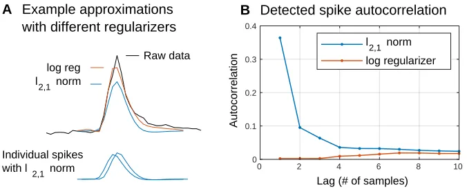
Figure 2.2: Issues with the convexl2,1regularizer. (A)The black trace shows a single
spike from a single channel of data. Overlaid are the optimal approximationsAxusing the
nonconvex log regularizer (red) and the convexl2,1norm (blue). Regularization withl2,1norm leads to two issues. First, the approximation is biased towards zero since the regularizer is always trying to shrink the feature vector norm. The log regularizer mitigates this by having a flatter slope for larger norms; note how the red trace captures more of the spike energy than the blue trace. Second, thel2,1 norm does nothing to discourage spikes from being split across consecutive time steps. In fact, this blue trace is actually the sum of two smaller spikes detected at consecutive time samples (bottom).(B)Autocorrelations of the detected
spike times. More than a third of the spikes detected using thel2,1norm (blue) are followed by another spike immediately afterwards (i.e., at a lag of 1). Such cases make it hard to interpret the deconvolution solution as a set of detected spikes. However, switching to the log regularizer (red) eliminates this problem.
is simply the sum of the column norms, there is no penalty to splitting a spike across
consecutive time steps. That is, from the regularizer’s point of view, there is no difference between x1and x2below:
x1=
h
· · · ξ 0 · · · i
x2=
h
· · · λξ (1−λ)ξ · · · i,
whereξ ∈RD and 0≤ λ≤ 1. Even though x1is the sparser solution, the regularizer
has no incentive to choose it, andx2often results in lower approximation error since
it allows for a sort of linear interpolation (Figure 2.2A).
To discourage spikes from getting split up like this, we need to define the regularizer
so that x2 is more expensive than x2, i.e., g(x2) > g(x1). Unfortunately, this
necessarily implies that the regularizer is no longer convex. To see this, consider that
x2= λx1+(1−λ)x3, where x3=
h
· · · 0 ξ · · · i.
that
g(λx1+(1−λ)x3)> λg(x1)+(1−λ)g(x3),
thereforegcannot be convex.
A variety of nonconvex sparsity-encouraging regularizers have been proposed in the literature. One such regularizer is the log penalty (Candes, Wakin, and Boyd, 2008),
and applying this to the column norms gives us our final regularizer:
g(x)= T
Õ
t=1
αlog(x[:,t]
+α). (2.6)
α >0 is a parameter that controls the non-convexity of this regularizer; asα→ ∞,
this approaches the l2,1 norm3. Switching from the convex l2,1 norm (2.5) to the nonconvex log regularizer (2.6) eliminates the incidence of double-detected spikes
(Figure 2.2B).
However, our choice of regularizer is also constrained by computational
considera-tions. Candes, Wakin, and Boyd (2008) implemented this log-regularized
approxi-mation using a reweightedl1minimization scheme. This approach—which involves wrapping an outer loop around a convex version of the optimization problem—is
less than ideal. Instead, we will approach this nonconvex minimization directly by
deriving a closed-form expression for the proximal operator of our columnwise log
regularizer (2.6) in Chapter 4. The existence of a simple proximal operator enables
us to solve our optimization problem (2.1) using a variety of large-scale optimization
algorithms, which I will discuss in the next section.
Finally, let me close this section with a few remarks on nonconvex optimization.
Since it is nonconvex, we are not guaranteed to converge to the global minimum,
and may instead get caught in local minima. Based on numerical experiments, it
seems that we can improve the quality of our solutions by (1) starting with the
convex solution by settingα=∞, and (2) slowly ramping downαover the course of many iterations in a process loosely analogous to simulated annealing. I found
that this approach produced sparser solutions with less approximation error than the
reweightedl1minimization of Candes, Wakin, and Boyd (2008), and reached this
solution in far fewer iterations.
3I will note that equation (2.6) differs slightly from previous work by the addition of factor ofα
15
0 500 1000 1500 2000
10-5
100
Objective value
Comparison of optimization algorithms
0 500 1000 1500 2000
0 1 2 3
Density
# of convolution operations ADMM Gradient descent Accelerated (FISTA)
Figure 2.3: Comparison of optimization algorithms. Comparison of three algorithms—
alternating directions method of multipliers (ADMM, yellow), proximal gradient descent (blue), and a form of accelerated proximal gradient descent (FISTA, red)—on a convex deconvolution problem. Runtime is measured in terms of the number of convolution operations, which is the most computationally intensive step. Top: Relative objective value JJ((xx)−J(x?)
0)−J(x?), where
J(x)is the objective function(2.1),x0is the starting point, and x?is the optimal solution as determined by running the algorithms for several thousand more iterations. Bottom:Relative
densitynnz(x)/nnz(x?), wherennz(x)is the number of nonzero entries inx.
2.2.5 Optimization algorithm
Figure 2.3 compares the performance4 of three popular optimization algorithms:
alternating direction method of multipliers (ADMM, yellow), proximal gradient
descent (blue), and a form of accelerated gradient descent known as the fast iterative shrinkage-thresholding algorithm (FISTA, red).
ADMM (Boyd et al., 2011) is a very popular optimization algorithm that has shown
promising results in a variety of difficult optimization problems (Swaminathan and
Murray, 2014; Horowitz, Papusha, and Burdick, 2014). It has attracted considerable
attention for deconvolution applications (Bristow, Eriksson, and Lucey, 2013; Heide,
Heidrich, and Wetzstein, 2015; Wohlberg, 2016; Wang et al., 2018) because the
proximal operator of the approximation error f(x) has a simple expression in frequency domain. However, since the proximal operator for the regularizerg(x)still must be evaluated in time domain, this does not actually reduce the number of FFT
4As a disclaimer, note that these results are for a different sparse deconvolution problem, involving
a larger set of kernels spanning a wide range of frequencies, and using the convexl1 regularizer.
operations per iteration as compared to gradient-based methods, and furthermore
precludes the use of the overlap-add technique to replace a large FFT with several smaller transforms. Ignoring this last concern, this procedure requires the equivalent
of two convolution operations per iteration.
Proximal gradient descent (Parikh and Boyd, 2014) is an extension of standard
gradient descent techniques to cases where the objective function may be written as
the sum of a smooth term f(x)and a potentially nonsmooth termg(x)that admits a simple proximal operator. This requires at least two convolutions per iteration, but
sometimes more due to backtracking5, and averaged 2.3 convolutions per iteration.
FISTA (Beck and Teboulle, 2009) is a form of accelerated gradient descent (see
Becker, Candès, and Grant, 2011, for an excellent overview), which adds a
momentum-like term that can help speed up convergence. I tried a variety of accelerated gradient
methods (Nesterov, 2013; Lan, Lu, and Monteiro, 2011; Auslender and Teboulle,
2006) and found their performance to be essentially identical (note that computing
the gradient is far more expensive than evaluating proxgin this problem). FISTA
was the easiest to implement and the most memory-efficient. This averaged 3.8
convolutions per iteration.
Despite requiring more convolutions per iteration, FISTA still converges much faster
than the other algorithms tested (Figure 2.3, top). More importantly, it arrives at a
sparse solution much sooner than the others (Figure 2.3, bottom). Here we see that
the accelerated algorithm produces a solution with near-optimal sparsity within 500
operations, while ADMM and gradient descent still contain twice as many nonzero
entries. Even after 2000 operations, these non-accelerated methods still contain
substantially more nonzero entries than optimal.
Using FISTA as the optimization algorithm, I could handle problem sizes up to
T = 1 million before running out of GPU memory. Since typical chronic datasets
5Backtracking is a way of automatically adjusting the step size. If a certain condition is not met,
then we backtrack, i.e., reduce the step size (by increasing our Lipschitz constant estimateL) and try again. While we are on this topic, note that the usual backtracking termination criterion
f(xi+1) ≤ f(xi)+h∇f(xi),xi+1−xii+
Li
2 kxi+1−xik
2
suffers from numerical cancellation issues since f(xi)and f(xi+1)may be much larger than the other
terms in this expression. But since f(x)=1
2kAx−bk 2
w, this is equivalent to
17
0 0.2 0.4 0.6 0.8 1 1.2 1.4
0 20 40 60 80
100 Spike-sorting performance on overlapping spikes
Inter-spike interval (ms)
True positive rate (%) Traditional spike detection 0.2 7.6
Sparse deconvolution 0.3 3.1
+ overlap reassignment 0.5 0.8 FP% FN%
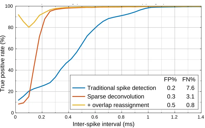
Figure 2.4: Spike detection performance on a hybrid ground truth dataset. Fraction of
donor spikes that were detected and assigned to the correct source (true positive rate) as a function of the time between spikes (inter-spike interval). The overall false discovery rate (FP%) and false negative rate (FN%) for each method are reported in the legend.
range from 100 million to a few billion samples in duration, I processed these datasets
in chunks and merged them together.
2.3 Results
To evaluate the spike detection performance, I created a “hybrid ground truth” dataset
(section 3.4.3) by adding known “donor” spikes to a relatively quiet recording. We
can then perform spike detection and clustering and measure the number of donor
spikes that were detected and assigned to the correct source (Figure 2.4).
Traditional spike detection using the nonlinear energy operator as the detection
heuris-tic and PCA for dimensionality reduction (blue) performs well on non-overlapping
spikes, but struggles with spikes that are less than 1 ms apart. Since this dataset
contains a high incidence of overlapping spikes, this results in an overall false negative rate of 7.6%.
The sparse deconvolution approach presented in this chapter (red) is able to reliably
deconvolve spikes down to 0.3 ms (for reference, the data shown in figure 2.1 shows
a pair of spikes separated by 0.3 ms), reducing the false negative rate by more than half. Remarkably, it is able to deconvolve these spikes without any clustering or
other characterization of the spike sources.
Raw data
LFP
A Spikes distort the LFP
0.5 mV 20 ms
With spikes Despiked
Ripple
band -20
-10 0 10 20
-180 -90 0 90 180
Phase shift (deg) due to spikes
Despiked ripple phase (deg)
C Shift in estimated ripple phase
-180 -90 0 90 180
Despiked ripple phase (deg) Number of spikes
B Ripple phase-locking for an example single unit
Ripple phase (deg)
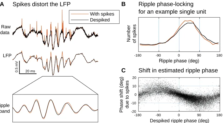
Figure 2.5: Spike removal for LFP analysis.Failing to remove spikes may bias subsequent
analysis of the local field potential (LFP).(A)Top: After detecting spikes using our approach,
these spikes can be removed from the original raw data (red) to produce a despiked signal (black).Middle:This broadband data is lowpass filtered to obtain an estimate of the LFP, a
measure of aggregate network activity. However, if spikes are not removed prior to filtering, then they will distort our LFP estimate. Bottom: A close-up after filtering in the ripple band
(100–200 Hz). Note that failing to remove spikes has changed the amplitude and phase of the observed ripple. (B)Ripple phase-locking analysis for a single unit (a putative CA1
interneuron), showing the histogram of spikes according to the phase of the ripple oscillation, as estimated from despiked LFP (black) and a with-spikes LFP (red). Note that the peak of the with-spikes histogram is narrower and shifted towards zero. (C)Shift in the estimated
ripple phase due to the presence of spikes. Each dot corresponds to a single spike from the unit in panel B, and shows the phase shiftθwith-spikes−θdespiked(i.e., the difference between
the despiked and with-spikes estimates of ripple phase) as a function of the ripple phase at which this spike was observed. This shows that the with-spikes LFP consistently biases the estimate of ripple phase towards zero.
from one very large spike. Resolving closely-overlapping spikes inevitably requires
some model of the individual sources (i.e., some idea of what the spikes produced by each putative neuron will look like). One approach, described in section 3.5,
augments the fitted model with additional components that correspond to overlap
between pairs of neurons at various lags. This overlap reassignment procedure
(yellow) is able to correctly reassign most of these closely-overlapping spikes based
only on their feature space representation (i.e., without recourse to the raw data),
bringing the overall false negative below 1%.
19
filtered and downsampled to form an estimate of the local field potential (LFP).
However, spikes still contain a fair amount of energy at lower frequencies, and this lowpass filtering does not completely remove their influence on the recorded signal
(Figure 2.5A). Instead, our spike detection method allows us to analyze the residual
b− Ax as a “despiked” version of the recorded signal. This is particularly relevant for the analysis of ripples (LFP oscillations in the range of 100–200 Hz), where
the activity of ripple-phase-locked neurons may produce consistent biases in the
apparent phase and amplitude of ripple oscillations (Figure 2.5B and C).
2.4 Discussion
In this chapter, I have presented a spike detection algorithm that follows the modular
approach of traditional spike detection—producing a feature-space representation of
the detected spikes without requiring any information about the clusters present in the recording—while offering improved resolution of overlapping spikes.
At the moment, the main drawback of this approach is that it is quite slow, running
only slightly faster than realtime on tetrode data (an hour-long recording takes nearly
one hour to process). Although the current software implementation has some room
for improvement, that alone cannot produce the 10 or 100x speedup that would be
necessary for large-scale deployment of this technique. Instead, a greedy approach
such as orthogonal matching pursuit (Pati, Rezaiifar, and Krishnaprasad, 1993) may
be more appropriate.
Finally, I will note that the generality of this technique—the fact that, aside from the
choice of spike basis waveforms, nothing ties this approach to the specific problem
of spike detection—allows us to consider using this approach for the detection and
C h a p t e r 3
SPIKE SORTING USING A MIXTURE OF DRIFTING
T
-DISTRIBUTIONS
Shan, K. Q., E. V. Lubenov, and A. G. Siapas (2017). “Model-based spike sorting with a mixture of drifting t-distributions”.Journal of neuroscience methods288, pp. 82–98. doi:10.1016/j.jneumeth.2017.06.017.
This chapter is based on previously-published material. In preparing this chapter, I
have condensed and rearranged the sections to be more amenable to selective reading.
I have also expanded section 3.5 to include results using a sparse deconvolution
approach to spike detection.
Section 3.1 provides some additional background on the spike sorting problem.
Section 3.2 describes the MoDT model and performs some benchmarking of our
software implementation of the model fitting algorithm. Section 3.3 evaluates the
model on several thousand hours of chronic tetrode recordings to show that it fits the empirical data substantially better than a mixture of Gaussians. Section 3.4
then demonstrates that the MoDT-based estimate of misclassification error is more
accurate than previous unit isolation metrics, and Section 3.5 discusses the issue of
temporally overlapping spikes.
3.1 Introduction
Chronic extracellular recordings offer access to the spiking activity of neurons over
the course of days or even months. However, the analysis of extracellular data
requires a process known as spike sorting, in which extracellular spikes are detected
and assigned to putative sources. Despite many decades of development, there is no
universally-applicable spike sorting algorithm that performs best in all situations.
Approaches to spike sorting can be divided into two categories: model-based and
non-model-based (or non-parametric). In the model-based approach, one constructs
a generative model (e.g., a mixture of Gaussian distributions) that describes the
probability distribution of spikes from each putative source. This model may be used
for spike sorting by comparing the posterior probability that a spike was generated
21
A Feature space scatterplots
ch 1 ch 2 ch 3 ch 4
B Spike waveforms
0 1 2 3 4 5
Time (hr)
C Cluster location over time
0 2 4 6 8
Mahalanobis distance
D Deviation from cluster center
ch 4
ch 1
Gauss
t-dist
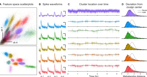
Figure 3.1: Extracellular recordings contain drifting, heavy-tailed clusters.(A)
Scatter-plots of spikes in feature space, color-coded by putative identity. Spike waveforms recorded on 4 tetrode channels were projected onto a 12-dimensional feature space using 3 principal components from each channel. Top: scatterplot of the first principal component from chan-nels 1 and 4. Bottom: a different projection of the data, showing only the best-isolated single units. (B) Spike waveforms (inverted polarity) for six example units. Scale bar: 200 µV, 0.5
ms. (C) Cluster drift in feature space. y-axis shows one of the 12 feature space dimensions. Black line indicates the cluster center fitted using the MoDT model. (D) Distribution of the
non-squared Mahalanobis distance (δ) from the fitted cluster center to the observed spikes. Lines indicate the theoretical distributions for Gaussian andt-distributed spikes.
maximum likelihood or Bayesian methods, and the model also provides an estimate
of the misclassification error.
In the non-parametric approach, spike sorting is treated solely as a classification problem. These classification methods may range from manual cluster cutting to
a variety of unsupervised learning algorithms. Regardless of the method used,
scientific interpretation of the sorted spike train still requires reliable, quantitative
measures of unit isolation quality. Often, these heuristics either explicitly (Hill,
Mehta, and Kleinfeld, 2011) or implicitly (Schmitzer-Torbert et al., 2005) assume
that the spike distribution follows a mixture of Gaussian distributions.
a slow change in the shape and amplitude of recorded waveforms (Figure 3.1C),
usually ascribed to motion of the recording electrodes relative to the neurons (Snider and Bonds, 1998; Lewicki, 1998). This effect may be small for short recordings
(< 1 hour), but can produce substantial errors if not addressed in longer recordings
(Figure 3.6). Even in the absence of drift, spike residuals have heavier tails than
expected from a Gaussian distribution, and may be better fit using a multivariate
t-distribution (Figure 3.1D and Figure 3.5; see also Shoham, Fellows, and Normann, 2003; Pouzat et al., 2004).
To address these issues, we model the spike data as a mixture of driftingt-distributions (MoDT). This model builds upon previous work that separately addressed the issues
of cluster drift (Calabrese and Paninski, 2011) and heavy tails (Shoham, Fellows, and
Normann, 2003), and we have found the combination to be extremely powerful for
modeling and analyzing experimental data. We also discuss the model’s robustness
to outliers, provide a software implementation of the fitting algorithm, and discuss
some methods for reducing errors due to spike overlap.
We used the MoDT model to perform spike sorting on 34,850 tetrode-hours of
chronic tetrode recordings (4.3 billion spikes) from the rat hippocampus, cortex, and cerebellum. Using these experimental data, we evaluate the assumptions of our model
and provide recommended values for the model’s user-defined parameters. We also
analyze how the observed cluster drift may impact the performance of spike sorting
methods that assume stationarity. Finally, we evaluate the accuracy of MoDT-based
estimates of misclassification error and compare this to the performance of other
popular unit isolation metrics in the presence of empirically-observed differences in
23
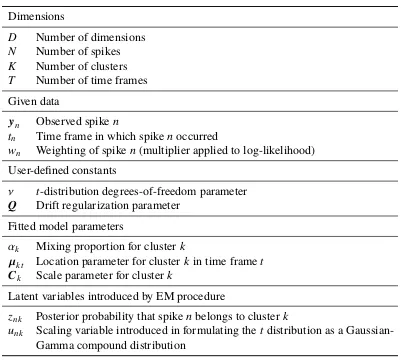
Table 3.1: Mathematical notation.Lowercase bold letters (yn,µkt) denoteD-dimensional
vectors, and uppercase bold letters (Ck,Q) denoteD×Dsymmetric positive definite matrices.
Dimensions
D Number of dimensions
N Number of spikes
K Number of clusters
T Number of time frames Given data
yn Observed spiken
tn Time frame in which spikenoccurred
wn Weighting of spiken(multiplier applied to log-likelihood)
User-defined constants
ν t-distribution degrees-of-freedom parameter Q Drift regularization parameter
Fitted model parameters
αk Mixing proportion for clusterk
µkt Location parameter for clusterk in time framet
Ck Scale parameter for clusterk
Latent variables introduced by EM procedure
znk Posterior probability that spikenbelongs to cluster k
unk Scaling variable introduced in formulating thet distribution as a
Gaussian-Gamma compound distribution
3.2 Mixture of driftingt-distributions (MoDT) model
In this section, I will introduce the mixture of driftingt-distributions (MoDT) model (section 3.2.1), describe an EM algorithm for fitting this model (section 3.2.2), and
analyze the computational scaling of this algorithm (section 3.2.3). Section 3.2.4
contains some stray remarks about how the multivariatet-distribution may be used for robust covariance estimation. Finally, section 3.2.5 discusses some potential
extensions to this MoDT model.
3.2.1 Model description
Spike sorting begins with spike detection and feature extraction. During these preprocessing steps, spikes are detected as discrete events in the extracellular voltage
trace and represented as points ynin someD-dimensional feature space.
drawn from a mixture distribution with PDF given by
fMoG(yn;φ)= K
Õ
k=1
αkfmvG(yn;µk,Ck),
whereφ = {. . . , αk,µk,Ck, . . .} is the set of fitted parameters,K is the number of mixture components,αkare the mixing proportions, and fmvG(y;µ,C)is the PDF of
the multivariate Gaussian distribution with mean µand covarianceC:
fmvG(y;µ,C)= 1
(2π)D/2|C|1/2exp
−1
2δ
2(y;µ,C)
.
For notational convenience, letδ2denote the squared Mahalanobis distance
δ2(y;µ,C)=(y−µ)|
C−1(y−µ).
We make two changes to this model. First, we replace the multivariate Gaussian
distribution with the multivariate t-distribution. The PDF for this distribution, parameterized by locationµ, scaleC, and degrees-of-freedomν, is given by
fmvt(y;µ,C, ν)
1
(νπ)D/2|C|1/2
Γ(ν+D
2 )
Γ(ν
2)
1+ 1
νδ2(y;µ,C)
−ν+2D
.
Second, we break up the dataset into T time frames (we used a frame duration of 1 minute) and allow the cluster location µ to change over time. The mixture
distribution becomes
fMoDT(yn;φ, ν)= K
Õ
k=1
αkfmvt(yn;µktn,Ck, ν),
where tn ∈ {1, . . . ,T} denotes the time frame for spike n. We use a common ν
parameter for all components and have chosen to treat it as a user-defined constant.
The fitted parameter set is thusφ= {. . . , αk,µk1, . . . ,µkT,Ck, . . .}.
In order to enforce consistency of the component locations across time, we introduce
a prior on the location parameter that penalizes large changes over consecutive time
steps. This prior has a joint PDF proportional to
fprior(µk1, . . . ,µkT)= T
Ö
t=2
fmvG(µkt − µk(t−1);0,Q), (3.1)
where Qis a user-defined covariance matrix that controls how much the clusters are
25
3.2.2 EM algorithm for model fitting
Assuming independent spikes and a uniform prior on the other model parameters,
we can obtain the maximuma posteriori(MAP) estimate of the fitted parametersφ by maximizing the log-posterior, which is equivalent (up to an additive constant) to
the following:
L(φ)= N
Õ
n=1
wnlog fMoDT(yn;φ)+ K
Õ
k=1
log fprior(µk1, . . . ,µkT).
Note that we have introduced a weightwnfor each spike. This allows us to fit the
model to a weighted subset of the data while remaining consistent with the full
dataset (Feldman, Faulkner, and Krause, 2011).
As with most mixture distributions, it is intractable to optimizeL(φ)directly. However, by introducing additional latent random variables, we obtain a “complete-data”
log-posterior Lc(φ,Z,U)that allows us to decompose the problem and optimize it using
an expectation-maximization (EM) algorithm (McLachlan and Peel, 2000).
In the E-step, we compute the expected value of Lc assuming that these latent
variables follow their conditional distribution given the observed data and the fitted parameters ˆφfrom the previous EM iteration. The conditional expectations of these
latent variables are given by:
znk =
ˆ
αkfmvt(yn; ˆµktn,Cˆk, ν)
Í
καˆκfmvt(yn; ˆµκtn,Cˆκ, ν)
, (3.2)
unk =
ν+D
ν+δ2(y
n; ˆµktn,Cˆk)
. (3.3)
The znk correspond to the posterior probability that spike n was produced by
componentk, and may thus be interpreted as a soft-assignment of spikes to clusters (i.e., putative neurons). The unk arises from the formulation of thet-distribution
as a Gaussian-Gamma compound distribution and may be interpreted as a scaling
variable that “Gaussianizes” the multivariatet-distribution. In the Gaussian case (the limit of at-distribution asν → ∞), we haveunk =1 for all spikes. For finiteν,
note thatunk decreases as the Mahalanobis distanceδ increases.
Next we can compute the conditional expectation of Lc(φ,Z,U) over these latent
to an additive constant) to
J(φ; ˆφ)= N
Õ
n=1 wn
K
Õ
k=1 znk
"
logαk − 1
2log|Ck| − 1 2unkδ
2(y
n;µktn,Ck)
#
+
T
Õ
t=2
−1
2δ
2(µ
kt −µk(t−1);0,Q).
In the M-step, we maximizeJ(φ,φˆ)with respect to the fitted parameters. The optimal value for the mixing proportionsαis simply a weighted version of the mixture of
Gaussians (MoG) M-step update:
arg max
αk
J(φ; ˆφ)= Í
nwnznk
Í
nwn
. (3.4)
The optimal value for the cluster scale parameter Cis also similar to the MoG case,
but each spike is additionally scaled byunk:
arg max
Ck
J(φ; ˆφ)= Í
nwnznkunk(yn− µktn)(yn− µktn)
|
Í
nwnznk
. (3.5)
For the cluster location parametersµ, note that J(φ,φˆ)is quadratic with respect toµ and its maximum occurs where the gradient∇µJ(φ,φˆ)= 0. We can therefore find the optimal µby solving the following linear system of equations:
∇µ
kJ(φ,φˆ)=
bk1
bk2
... bkT − A
µk1
µk2
... µkT
=0, (3.6)
where A=
Mk1+Q
−1
−Q−1
−Q−1 Mk2+2Q
−1
−Q−1
−Q−1 . . . .
. . . MkT +Q
−1 and
Mkt = C
−1
k
Õ
n:tn=t
wnznkunk
bkt = C
−1
k
Õ
n:tn=t
27
EM fitting of the MoDT model thus consists of iterative evaluation of equations (3.2)
through (3.6). A few remarks on this procedure:
1. Most of theznk end up very close to zero, and ignoring these spikes in the
M-step can reduce the complexity of that operation. However, the sparsity needs to be very high (K > 20, as a rule of thumb) to outweigh the efficiency advantages of the highly-optimized numerical routines for dense linear algebra.
We found that applying a threshold onznk produced more accurate results than
“hard EM” (in which each spike is assigned to only one cluster), which tends
to underestimate the covariance of highly-overlapping clusters.
2. The scaling variableunkacts as an additional weighting term in the optimization
ofµ andC. Sinceunk decreases as spikengets far away from cluster k, any
outliers are automatically discounted during the fitting process. As a result, the
fitted parameters are considerably more robust to the presence of outliers than in the Gaussian case (Lange, Little, and Taylor, 1989; Peel and McLachlan,
2000).
3. The optimal value ofµdepends on the value ofCand vice-versa. Although the
standard EM algorithm calls for maximizingJ(φ,φˆ)over allφ, the convergence of a generalized EM algorithm requires only that we improve upon the previous
ˆ
φ(Dempster, Laird, and Rubin, 1977). Therefore we need not simultaneously optimizeµandC, but may instead update them one at a time.
4. Although equation (3.6) involves solving aDT×DTlinear system, its sparsity structure allows us to solve forµwith a complexity that scales linearly with
T. For example, Mkt and bkt appear in theinformation filter, an alternative
paramaterization of the Kalman filter (see, e.g., Anderson and Moore, 1979).
The acausal problem can then be solved using a backwards pass (Rauch, Tung,
and Striebel, 1965). However, we have found that it is faster to solve equation
(3.6) using standard numerical linear algebra routines for solving banded
positive semi-definite matrices (i.e., LAPACKdpbsv).
3.2.3 Software implementation and computational scaling
A MATLAB implementation of this EM algorithm, along with a demo script, is
available athttps://github.com/kqshan/MoDT. In this section, we measure the
runtime on a desktop workstation with an Intel Core i5-7500 CPU, 32 GB of memory,
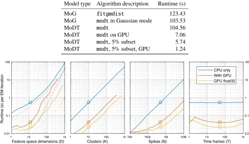
Table 3.2: Computational runtime for model fitting.Time required to perform 20 EM
itera-tions on the sample dataset shown in Figure 3.1 (D=12, K=26, N=1.9 million).fitgmdistis a mixture of Gaussians fitting routine that is part of the MATLAB Statistics and Machine Learning Toolbox.modtis a MATLAB implementation of our EM algorithm that may be downloaded
fromhttps://github.com/kqshan/MoDT. In addition to fitting the richer MoDT model, it
supports two additional features (data weights and GPU computing) that can dramatically reduce fitting times.
Model type Algorithm description Runtime (s)
MoG fitgmdist 123.43
MoG modtin Gaussian mode 103.53
MoDT modt 104.56
MoDT modton GPU 7.06
MoDT modt, 5% subset 5.74
MoDT modt, 5% subset, GPU 1.24
1 10 100 1k
Feature space dimensions (D)
0.01 0.1 1 10 100
Runtime (s) per EM iteration
1 10 100 1k
Clusters (K) 10k 100kSpikes (N)1M 10M 1 Time frames (T)10 100 1k
0.01 0.1 1 10 100
CPU only With GPU GPU, 32-bit
GPU float32
Figure 3.2: Scaling of computational runtime with model dimensions. Starting from a
baseline ofD= 12,K= 10,N= 500,000,T= 50, we varied each dimension and measured the
runtime on CPU (blue) and GPU (red). We also measured GPU runtime using single-precision (32-bit floating point) arithmetic (yellow). ForD, we show the theoretical limits imposed by
the hardware’s computing power (dashed line) and memory throughput (dotted line). Peak memory usage is(5K+4D)Nelements, and the GPU line ends when we run out of GPU
memory (8 GB).
Our implementation offers a mild speedup over the MATLAB built-in mixture-of-Gaussians fitting routine, despite fitting a more complex model (Table 3.2). In
addition, it supports the use of a weighted training subset, which offers a proportional
reduction in runtime at the expense of model accuracy, and supports the use of GPU
computing using the NVidia CUDA computing platform.
29
most computationally intensive operations are computing the Mahalanobis distance
(D2K N), updating the cluster location µ(DK N+ D3KT), and updating the scale parameterC (D2K N). Since the number of spikes is typically much larger than the number of time frames or dimensions (N DT), we expect the fitting time to scale asD2K Noverall. To test these scaling laws, we measured the runtime while varying each model dimension (Figure 3.2).
Surprisingly, we found that the CPU runtime scaled almost linearly withD. This is because the CPU’s memory throughput (17 GB/s), rather than its computing power
(218 GFLOPS), is the limiting factor1 whenD < 500, and memory access scales linearly withD.
The GPU’s higher memory throughput (320 GB/s) affords a substantial speedup on
smallD. Like many consumer-grade GPUs, this device’s single-precision computing power (8.2 TFLOPS) is substantially higher than its double-precision capacity
(257 GFLOPS), and switching to single-precision arithmetic dramatically increases
performance on compute-limited tasks.
As expected, we found the runtime scales linearly with KandN, and the effect ofT
is negligible. The GPU shows similar trends, but with reduced efficiency at small N
andT due to poor utilization of the hardware resources.
Finally, we measured the peak memory usage to be approximately 5N ×K matrices and 4D×N matrices, for a total of 8(5K+4D)N bytes (double-precision). Fitting larger datasets may require using a weighted subset of spikes and/or performing the
optimization in batches.
3.2.4 Robust covariance estimation using thet-distribution
In this section, let us take a brief intermission from our consideration of drifting,
heavy-tailed data and look at the case where the underlying data are stationary and Gaussian, but unmodeled noise or artifacts may be present. In such cases,
standard estimates of the data covariance may be unduly influenced by these outliers
(Figure 3.3A). Since the data covariance is a critical component of multivariate
statistics, it is important to have a covariance estimator that is robust to the presence
of outliers.
One very popular robust covariance estimator is the minimum covariance determinant
(MCD) estimator (Rousseeuw and Driessen, 1999). In this approach, the data points
Using Gaussian Using ν=10
True distribution
A B
Figure 3.3: Robust covariance estimation using thet-distribution. Thet-distribution
may also be used to derive robust estimates of Gaussian parameters. In this example, we generated 100 points from a Gaussian distribution and added a single outlier (red arrow). (A)
This has stretched out the estimated covariance when using a Gaussian fit. (B)The fitted
t-distribution is largely unaffected by the outlier. Equation(3.7)can then be used to convert the fittedt-distribution scale parameter into an equivalent Gaussian covariance parameter.
are weighted according to their distance from the estimated center—specifically,
points with a Mahalanobis distance below some threshold are given a weight of 1
and points beyond that threshold are given a weight of 0—and then the weighted
covariance is multiplied by a correction factor to achieve consistency with an
non-truncated Gaussian distribution. Finding the appropriate set of points to include
in this estimate requires an iterative procedure, preferably with multiple random
initializations, and may be very slow to converge when there are many data points.
As we noted in the previous section, fitting the multivariate t-distribution also discounts any points that are far away from the estimated center. In Figure 3.3B, we
have fit this same dataset using at-distribution, and we can see that it automatically rejects the influence of the outlier. However, this has also caused us to overestimate
the distribution tails: note how the fitted t-distribution’s 99% confidence ellipse (green) is inflated relative to the true ellipse (black).
Rather than using thet-distribution directly, can we use the fitted parameters µand Cto derive robust estimates of the Gaussian mean and covariance? As the number of
samplesN → ∞, the fittedµconverges to the Gaussian distribution’s true mean, but the fittedC is a biased estimator of the Gaussian distribution’s covariance parameter.
However, we can compute a correction factor by solving for βin
∫ ∞
0
ν+D
βν+xx
D/2e−x/2dx =2D/2Γ(D/2)D, (3.7)
and then useβCas a robust estimate for the Gaussian covariance. The corresponding
99% confidence ellipse is also plotted in Figure 3.3B as a light grey ellipse, but it is
![Table 2.1: Mathematical notation. For a [D × T] matrix x, the notation x[d,:] refers to itsd-th row and x[:,t] refers to its t-th column.](https://thumb-us.123doks.com/thumbv2/123dok_us/1130312.1141729/15.612.108.507.101.468/table-mathematical-notation-matrix-notation-refers-refers-column.webp)