Human Language Technologies: The 2009 Annual Conference of the North American Chapter of the ACL, pages 468–476,
Shrinking Exponential Language Models
Stanley F. Chen
IBM T.J. Watson Research Center P.O. Box 218, Yorktown Heights, NY 10598
Abstract
In (Chen, 2009), we show that for a vari-ety of language models belonging to the ex-ponential family, the test set cross-entropy of a model can be accurately predicted from its training set cross-entropy and its parameter values. In this work, we show how this rela-tionship can be used to motivate two heuristics for “shrinking” the size of a language model to improve its performance. We use the first heuristic to develop a novel class-based lan-guage model that outperforms a baseline word trigram model by 28% in perplexity and 1.9% absolute in speech recognition word-error rate on Wall Street Journal data. We use the second heuristic to motivate a regularized version of minimum discrimination information models and show that this method outperforms other techniques for domain adaptation.
1 Introduction
An exponential modelpΛ(y|x)is a model with a set
of features{f1(x, y), . . . , fF(x, y)}and equal num-ber of parametersΛ ={λ1, . . . , λF}where
pΛ(y|x) =
exp(PF
i=1λifi(x, y)) ZΛ(x)
(1)
and where ZΛ(x) is a normalization factor. In
(Chen, 2009), we show that for many types of ex-ponential language models, if a training and test set are drawn from the same distribution, we have
Htest≈ Htrain+
γ D
F X
i=1
|λ˜i| (2)
whereHtestdenotes test set cross-entropy;Htrain
de-notes training set cross-entropy;Dis the number of events in the training data; theλ˜iare regularized pa-rameter estimates; andγ is a constant independent
of domain, training set size, and model type.1 This relationship is strongest if the ˜Λ = {˜λi} are esti-mated using`1+`22regularization (Kazama and
Tsu-jii, 2003). In`1+`22 regularization, parameters are
chosen to optimize
O`1+`22(Λ) =Htrain+
α D
F X
i=1 |λi|+
1 2σ2D
F X
i=1 λ2i (3)
for some α and σ. With (α = 0.5, σ2 = 6)and takingγ = 0.938, test set cross-entropy can be pre-dicted with eq. (2) for a wide range of models with a mean error of a few hundredths of a nat, equivalent to a few percent in perplexity.2
In this paper, we show how eq. (2) can be applied to improve language model performance. First, we use eq. (2) to analyze backoff features in exponential
n-gram models. We find that backoff features im-prove test set performance by reducing the “size” of a modelD1 PFi=1|˜λi|rather than by improving train-ing set performance. This suggests the followtrain-ing principle for improving exponential language mod-els: if a model can be “shrunk” without increasing its training set cross-entropy, test set cross-entropy should improve. We apply this idea to motivate two language models: a novel class-based language model and regularized minimum discrimination in-formation (MDI) models. We show how these mod-els outperform other modmod-els in both perplexity and word-error rate on Wall Street Journal (WSJ) data.
The organization of this paper is as follows: In Section 2, we analyze the use of backoff features in
n-gram models to motivate a heuristic for model de-sign. In Sections 3 and 4, we introduce our novel
1The cross-entropy of a modelpΛ(y
|x)on some dataD= (x1, y1), . . . ,(xD, yD)is defined as−D1 PDj=1logpΛ(yj|xj).
It is equivalent to the negative mean log-likelihood per event as well as to log perplexity.
2A nat is a “natural” bit and is equivalent tolog
2eregular
bits. We use nats to be consistent with (Chen, 2009).
features Heval Hpred Htrain P|˜λi| D 3g 2.681 2.724 2.341 0.408 2g+3g 2.528 2.513 2.248 0.282 1g+2g+3g 2.514 2.474 2.241 0.249
Table 1: Various statistics for letter trigram models built on a 1k-word training set. Heval is the cross-entropy of the evaluation data;Hpredis the predicted test set cross-entropy according to eq. (2); and Htrain is the training set cross-entropy. The evaluation data is drawn from the same distribution as the training;Hvalues are in nats.
-4 -3 -2 -1 0 1 2 3 4 5
λ
[image:2.612.85.289.59.113.2]predicted letter
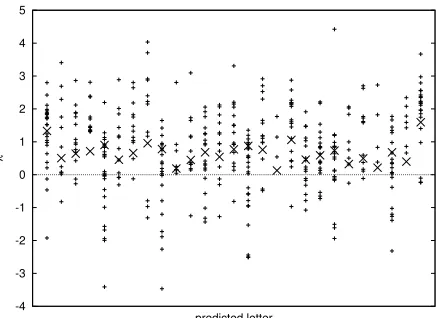
Figure 1: Nonzero˜λi values for bigram features in let-ter bigram model without unigram backoff features. If we denote bigrams aswj−1wj, each column contains the
˜
λi’s corresponding to all bigrams with a particularwj. The ‘×’ marks represent the average|λ˜i|in each column; this average includes history words for which no feature exists or for whichλ˜i= 0.
class-based model and discuss MDI domain adapta-tion, and compare these methods against other tech-niques on WSJ data. Finally, in Sections 5 and 6 we discuss related work and conclusions.3
2 N-Gram Models and Backoff Features
In this section, we use eq. (2) to explain why backoff features in exponentialn-gram models improve per-formance, and use this analysis to motivate a general heuristic for model design. An exponentialn-gram model contains a binary featurefωfor eachn0-gram
ω occurring in the training data forn0 ≤ n, where
fω(x, y) = 1iffxy ends inω. We refer to features corresponding to n0-grams for n0 < n as backoff features; it is well known that backoff features help
3
A long version of this paper can be found at (Chen, 2008).
-4 -3 -2 -1 0 1 2 3 4 5
λ
[image:2.612.74.296.210.370.2]predicted letter
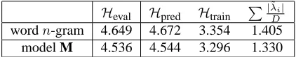
Figure 2: Like Figure 1, but for model with unigram backoff features.
performance a great deal. We present statistics in Table 1 for various letter trigram models built on the same data set. In these and all later experiments, all models are regularized with `1 +`22 regularization
with(α= 0.5, σ2 = 6). The last row corresponds to a normal trigram model; the second row corresponds to a model lacking unigram features; and the first row corresponds to a model with no unigram or bi-gram features. As backoff features are added, we see that the training set cross-entropy improves, which is not surprising since the number of features is in-creasing. More surprising is that as we add features, the “size” of the model D1 PFi=1|˜λi|decreases.
We can explain these results by examining a sim-ple examsim-ple. Consider an exponential model con-sisting of the featuresf1(x, y)andf2(x, y)with
pa-rameter values˜λ1 = 3andλ˜2 = 4. From eq. (1),
this model has the form
pΛ˜(y|x) =
exp(3f1(x, y) + 4f2(x, y)) ZΛ(x)
(4)
Now, consider creating a new feature f3(x, y) =
f1(x, y)+f2(x, y)and setting our parameters as
fol-lows:λnew
1 = 0,λnew2 = 1, andλnew3 = 3.
Substitut-ing into eq. (1), we see thatpΛnew(y|x) = pΛ˜(y|x)
for all x, y. As the distribution this model de-scribes does not change, neither will its training per-formance. However, the (unscaled) size PFi=1|λi| of the model has been reduced from 3+4=7 to 0+1+3=4, and consequently by eq. (2) we predict that test performance will improve.4
4
When sgn(˜λ1) =sgn(˜λ2),PF
In fact, since pΛnew = pΛ˜, test performance will
remain the same. The catch is that eq. (2) applies only to the regularized parameter estimates for a model, and in general, Λnew will not be the regu-larized parameter estimates for the expanded feature set. We can compute the actual regularized parame-ters ˜Λnewfor which eq. (2) will apply; this may im-prove predicted performance even more.
Hence, by adding “redundant” features to a model to shrink its total size PFi=1|λ˜i|, we can improve predicted performance (and perhaps also actual per-formance). This analysis suggests the following technique for improving model performance:
Heuristic 1 Identify groups of features which will
tend to have similarλ˜i values. For each such fea-ture group, add a new feafea-ture to the model that is the sum of the original features.
The larger the original˜λi’s, the larger the reduction in model size and the higher the predicted gain.
Given this perspective, we can explain why back-off features improve n-gram model performance. For simplicity, consider a bigram model, one with-out unigram backoff features. It seems intuitive that probabilities of the form p(wj|wj−1) are
sim-ilar across differentwj−1, and thus so are theλ˜ifor the corresponding bigram features. (If a word has a high unigram probability, it will also tend to have high bigram probabilities.) In Figure 1, we plot the nonzeroλ˜i values for all (bigram) features in a bi-gram model without unibi-gram features. Each column contains the˜λi values for a different predicted word
wj, and the ‘×’ mark in each column is the average value of |λ˜i| over all history wordswj−1. We see
that the average|λ˜i|for each wordwj is often quite far from zero, which suggests creating features
fwj(x, y) =
X
wj−1
fwj−1wj(x, y) (5)
to reduce the overall size of the model.
In fact, these features are exactly unigram backoff features. In Figure 2, we plot the nonzero˜λi values for all bigram features after adding unigram backoff features. We see that the average |λ˜i|’s are closer to zero, implying that the model sizePFi=1|λ˜i|has
settingλnew3 to theλ˜iwith the smaller magnitude, and the size
of the reduction is equal to|λnew3 |. If sgn(˜λ1)6=sgn(˜λ2), no
reduction is possible through this transformation.
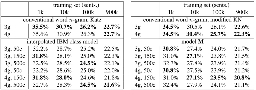
Heval Hpred Htrain P|
˜
λi| D wordn-gram 4.649 4.672 3.354 1.405
[image:3.612.321.532.60.101.2]model M 4.536 4.544 3.296 1.330
Table 2: Various statistics for word and class trigram models built on 100k sentences of WSJ training data.
been significantly decreased. We can extend this idea to higher-ordern-gram models as well; e.g., bi-gram parameters can shrink tribi-gram parameters, and can in turn be shrunk by unigram parameters. As shown in Table 1, both training set cross-entropy and model size can be reduced by this technique.
3 Class-Based Language Models
In this section, we show how we can use Heuris-tic 1 to design a novel class-based model that outper-forms existing models in both perplexity and speech recognition word-error rate. We assume a wordwis always mapped to the same classc(w). For a sen-tencew1· · ·wl, we have
p(w1· · ·wl) =Qlj+1=1p(cj|c1· · ·cj−1, w1· · ·wj−1)× Ql
j=1p(wj|c1· · ·cj, w1· · ·wj−1) (6)
wherecj = c(wj) and cl+1 is the end-of-sentence
token. We use the notationpng(y|ω)to denote an
ex-ponentialn-gram model, a model containing a fea-ture for each suffix of eachωyoccurring in the train-ing set. We usepng(y|ω1, ω2)to denote a model
con-taining all features inpng(y|ω1)andpng(y|ω2).
We can define a class-based n-gram model by choosing parameterizations for the distributions
p(cj| · · ·)andp(wj| · · ·)in eq. (6) above. For exam-ple, the most widely-used class-basedn-gram model is the one introduced by Brown et al. (1992); we re-fer to this model as the IBM class model:
p(cj|c1· · ·cj−1, w1· · ·wj−1)=png(cj|cj−2cj−1) p(wj|c1· · ·cj, w1· · ·wj−1)=png(wj|cj) (7)
(In the original work, non-exponentialn-gram mod-els are used.) Clearly, there is a large space of pos-sible class-based models.
and anothern-gramω0 created by replacing a word inω with a similar word, then the two correspond-ing features should have similar λ˜i’s. For exam-ple, it seems intuitive that then-grams on Monday morning and on Tuesday morning should have sim-ilar˜λi’s. Heuristic 1 tells us how to take advantage of this observation to improve model performance.
Let’s begin with a word trigram model
png(wj|wj−2wj−1). First, we would like to
convert this model into a class-based model. Without loss of generality, we have
p(wj|wj−2wj−1) =Pcjp(wj, cj|wj−2wj−1)
=Pcjp(cj|wj−2wj−1)p(wj|wj−2wj−1cj) (8)
Thus, it seems reasonable to use the distributions
png(cj|wj−2wj−1) andpng(wj|wj−2wj−1cj) as the starting point for our class model. This model can express the same set of word distributions as our original model, and hence may have a similar train-ing cross-entropy. In addition, this transformation can be viewed as shrinking together wordn-grams that differ only inwj. That is, we expect that pairs ofn-gramswj−2wj−1wj that differ only inwj (be-longing to the same class) should have similar λ˜i. From Heuristic 1, we can make new features
fwj−2wj−1cj(x, y) =
X
wj∈cj
fwj−2wj−1wj(x, y) (9)
These are exactly the features inpng(cj|wj−2wj−1).
When applying Heuristic 1, all features typically be-long to the same model, but even when they don’t one can achieve the same net effect.
Then, we can use Heuristic 1 to also shrink to-gethern-gram features forn-grams that differ only in their histories. For example, we can create new features of the form
fcj−2cj−1cj(x, y) =
X
wj−2∈cj−2,wj−1∈cj−1
fwj−2wj−1cj(x, y) (10)
This corresponds to replacing png(cj|wj−2wj−1)
with the distribution png(cj|cj−2cj−1, wj−2wj−1).
We refer to the resulting model as model M:
p(cj|c1···cj−1,w1···wj−1)=png(cj|cj−2cj−1,wj−2wj−1)
p(wj|c1···cj,w1···wj−1)=png(wj|wj−2wj−1cj) (11)
By design, it is meant to have similar training set cross-entropy as a wordn-gram model while being significantly smaller.
To give an idea of whether this model behaves as expected, in Table 2 we provide statistics for this model (as well as for an exponential wordn-gram model) built on 100k WSJ training sentences with 50 classes using the same regularization as before. We see that model M is both smaller than the baseline and has a lower training set cross-entropy, similar to the behavior found when adding backoff features to wordn-gram models in Section 2. As long as eq. (2) holds, model M should have good test performance; in (Chen, 2009), we show that eq. (2) does indeed hold for models of this type.
3.1 Class-Based Model Comparison
In this section, we compare model M against other class-based models in perplexity and word-error rate. The training data is 1993 WSJ text with verbal-ized punctuation from the CSR-III Text corpus, and the vocabulary is the union of the training vocabu-lary and 20k-word “closed” test vocabuvocabu-lary from the first WSJ CSR corpus (Paul and Baker, 1992). We evaluate training set sizes of 1k, 10k, 100k, and 900k sentences. We create three different word classings containing 50, 150, and 500 classes using the algo-rithm of Brown et al. (1992) on the largest training set.5 For each training set and number of classes, we build 3-gram and 4-gram versions of each model.
From the verbalized punctuation data from the training and test portions of the WSJ CSR corpus, we randomly select 2439 unique utterances (46888 words) as our evaluation set. From the remaining verbalized punctuation data, we select 977 utter-ances (18279 words) as our development set.
We compare the following model types: con-ventional (i.e., non-exponential) wordn-gram mod-els; conventional IBM class n-gram models in-terpolated with conventional word n-gram models (Brown et al., 1992); and model M. All conven-tional n-gram models are smoothed with modified Kneser-Ney smoothing (Chen and Goodman, 1998), except we also evaluate wordn-gram models with Katz smoothing (Katz, 1987). Note: Because word
5One can imagine choosing word classes to optimize model
training set (sents.) 1k 10k 100k 900k conventional wordn-gram, Katz 3g 579.3 317.1 196.7 137.5 4g 592.6 325.6 202.4 136.7
interpolated IBM class model 3g, 50c 358.4 224.5 156.8 117.8 3g, 150c 346.5 210.5 149.0 114.7 3g, 500c 372.6 210.9 145.8 112.3 4g, 50c 362.1 220.4 149.6 109.1 4g, 150c 346.3 207.8 142.5 105.2 4g, 500c 371.5 207.9 140.5 103.6
training set (sents.) 1k 10k 100k 900k conventional wordn-gram, modified KN 3g 488.4 270.6 168.2 121.5 4g 486.8 267.4 163.6 114.4
model M
[image:5.612.118.496.59.207.2]3g, 50c 341.5 210.0 144.5 110.9 3g, 150c 342.6 203.7 140.0 108.0 3g, 500c 387.5 212.7 142.2 108.1 4g, 50c 345.8 209.0 139.1 101.6 4g, 150c 344.1 202.8 135.7 99.1 4g, 500c 390.7 211.1 138.5 100.6
Table 3: WSJ perplexity results. The best performance for each training set for each model type is highlighted in bold.
training set (sents.)
1k 10k 100k 900k
conventional wordn-gram, Katz 3g 35.5% 30.7% 26.2% 22.7% 4g 35.6% 30.9% 26.3% 22.7%
interpolated IBM class model
3g, 50c 32.2% 28.7% 25.2% 22.5% 3g, 150c 31.8% 28.1% 25.0% 22.3% 3g, 500c 32.5% 28.5% 24.5% 22.1% 4g, 50c 32.2% 28.6% 25.0% 22.0% 4g, 150c 31.8% 28.0% 24.6% 21.8% 4g, 500c 32.7% 28.3% 24.5% 21.6%
training set (sents.)
1k 10k 100k 900k
conventional wordn-gram, modified KN 3g 34.5% 30.5% 26.1% 22.6% 4g 34.5% 30.4% 25.7% 22.3%
model M
3g, 50c 30.8% 27.4% 24.0% 21.7% 3g, 150c 31.0% 27.1% 23.8% 21.5% 3g, 500c 32.3% 27.8% 23.9% 21.4% 4g, 50c 30.8% 27.5% 23.9% 21.2% 4g, 150c 31.0% 27.1% 23.5% 20.8% 4g, 500c 32.4% 27.9% 24.1% 21.1%
Table 4: WSJ lattice rescoring results; all values are word-error rates. The best performance for each training set size for each model type is highlighted in bold. Each 0.1% in error rate corresponds to about 47 errors.
classes are derived from the largest training set, re-sults for word models and class models are compa-rable only for this data set. The interpolated model is the most popular state-of-the-art class-based model in the literature, and is the only model here using the development set to tune interpolation weights.
We display the perplexities of these models on the evaluation set in Table 3. Model M performs best of all (even without interpolating with a wordn-gram model), outperforming the interpolated model with every training set and achieving its largest reduction in perplexity (4%) on the largest training set. While these perplexity reductions are quite modest, what matters more is speech recognition performance.
For the speech recognition experiments, we use a cross-word quinphone system built from 50 hours of Broadcast News data. The system contains 2176 context-dependent states and a total of 50336 Gaus-sians. To evaluate our language models, we use
lat-tice rescoring. We generate latlat-tices on both our de-velopment and evaluation data sets using the Latt-AIX decoder (Saon et al., 2005) in the Attila speech recognition system (Soltau et al., 2005). The lan-guage model for lattice generation is created by building a modified Kneser-Ney-smoothed word tri-gram model on our largest training set; this model is pruned to contain a total of 350kn-grams using the algorithm of Stolcke (1998). We choose the acoustic weight for each model to optimize word-error rate on the development set.
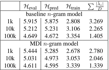
[image:5.612.95.519.240.389.2]Heval Hpred Htrain P|
˜
λi| D baselinen-gram model 1k 5.915 5.875 2.808 3.269 10k 5.212 5.231 3.106 2.265 100k 4.649 4.672 3.354 1.405
MDIn-gram model
[image:6.612.97.275.59.173.2]1k 5.444 5.285 2.678 2.780 10k 5.031 4.973 3.053 2.046 100k 4.611 4.595 3.339 1.339
Table 5: Various statistics for WSJ trigram models, with and without a Broadcast News prior model. The first col-umn is the size of the in-domain training set in sentences.
not a reliable predictor of speech recognition perfor-mance. While we can only compare class models with word models on the largest training set, for this training set model M outperforms the baseline Katz-smoothed word trigram model by 1.9% absolute.6
4 Domain Adaptation
In this section, we introduce another heuristic for improving exponential models and show how this heuristic can be used to motivate a regularized ver-sion of minimum discrimination information (MDI) models (Della Pietra et al., 1992). Let’s say we have a model pΛ˜ estimated from one training set and a
“similar” model q estimated from an independent training set. Imagine we useqas a prior model for
pΛ; i.e., we make a new modelpqΛnewas follows:
pqΛnew(y|x) =q(y|x)
exp(PF
i=1λnewi fi(x, y)) ZΛnew(x)
(12)
Then, chooseΛnewsuch thatpqΛnew(y|x) =pΛ˜(y|x)
for allx, y(assuming this is possible). Ifqis “simi-lar” topΛ˜, then we expect the sizeD1 PFi=1|λnewi |of
pqΛnewto be less than that ofpΛ˜. Since they describe
the same distribution, their training set cross-entropy will be the same. By eq. (2), we expect pqΛnew to
have better test set performance thanpΛ˜ after
reesti-mation.7In (Chen, 2009), we show that eq. (2) does indeed hold for models with priors; q need not be accounted for in computing model size as long as it is estimated on a separate training set.
6
Results for several other baseline language models and with a different acoustic model are given in (Chen, 2008).
7That is, we expect the regularized parametersΛ˜newto yield
improved performance.
This analysis suggests the following method for improving model performance:
Heuristic 2 Find a “similar” distribution estimated
from an independent training set, and use this distri-bution as a prior.
It is straightforward to apply this heuristic to the task of domain adaptation for language modeling. In the usual formulation of this task, we have a test set and a small training set from the same domain, and a large training set from a different domain. The goal is to use the data from the outside domain to max-imally improve language modeling performance on the target domain. By Heuristic 2, we can build a language model on the outside domain, and use this model as the prior model for a language model built on the in-domain data. This method is identical to the MDI method for domain adaptation, except that we also apply regularization.
In our domain adaptation experiments, our out-of-domain data is a 100k-sentence Broadcast News training set. For our in-domain WSJ data, we use training set sizes of 1k, 10k, and 100k sentences. We build an exponential n-gram model on the Broad-cast News data and use this model as the prior model
q(y|x)in eq. (12) when building an exponentialn -gram model on the in-domain data. In Table 5, we display various statistics for trigram models built on varying amounts of in-domain data when using a Broadcast News prior and not. Across training sets, the MDI models are both smaller inD1 PFi=1|λ˜i|and have better training set cross-entropy than the un-adapted models built on the same data. By eq. (2), the adapted models should have better test perfor-mance and we verify this in the next section.
4.1 Domain Adaptation Method Comparison
In this section, we examine how MDI adapta-tion compares to other state-of-the-art methods for domain adaptation in both perplexity and speech recognition word-error rate. For these experiments, we use the same development and evaluation sets and lattice rescoring setup from Section 3.1.
in-domain data (sents.) in-domain data (sents.)
1k 10k 100k 1k 10k 100k
in-domain data only
3g 488.4 270.6 168.2 34.5% 30.5% 26.1% 4g 486.8 267.4 163.6 34.5% 30.4% 25.7%
count merging
3g 503.1 290.9 170.7 30.4% 28.3% 25.2% 4g 497.1 284.9 165.3 30.0% 28.0% 25.3%
linear interpolation
3g 328.3 234.8 162.6 30.3% 28.5% 25.8% 4g 325.3 230.8 157.6 30.3% 28.4% 25.2%
MDI model
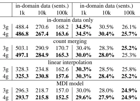
[image:7.612.66.307.68.241.2]3g 296.3 218.7 157.0 30.0% 28.0% 24.9% 4g 293.7 215.8 152.5 29.6% 27.9% 24.9%
Table 6: WSJ perplexity and lattice rescoring results for domain adaptation models. Values on the left are perplex-ities and values on the right are word-error rates.
in-domain and out-of-domain data are concatenated into a single training set, and a singlen-gram model is built on the combined data set. The in-domain data set may be replicated several times to more heavily weight this data. We also consider the base-line of not using the out-of-domain data.
In Table 6, we display perplexity and word-error rates for each method, for both trigram and 4-gram models and with varying amounts of in-domain training data. The last method corresponds to the exponential MDI model; all other methods employ conventional (non-exponential)n-gram models with modified Kneser-Ney smoothing. In count merging, only one copy of the in-domain data is included in the training set; including more copies does not im-prove evaluation set word-error rate.
Looking first at perplexity, MDI models outper-form the next best method, linear interpolation, by about 10% in perplexity on the smallest data set and 3% in perplexity on the largest. In terms of word-error rate, MDI models again perform best of all, outperforming interpolation by 0.3–0.7% absolute and count merging by 0.1–0.4% absolute.
5 Related Work
5.1 Class-Based Language Models
In past work, the most common baseline models are Katz-smoothed word trigram models. Compared to this baseline, model M achieves a perplexity
reduc-tion of 28% and word-error rate reducreduc-tion of 1.9% absolute with a 900k-sentence training set. The most closely-related existing model to model M is the model fullibmpredict proposed by Goodman (2001):
p(cj|cj−2cj−1,wj−2wj−1)=
λ p(cj|wj−2wj−1)+(1−λ)p(cj|cj−2cj−1)
p(wj|cj−2cj−1cj,wj−2wj−1)=
µ p(wj|wj−2wj−1cj)+(1−µ)p(wj|cj−2cj−1cj) (13)
This is similar to model M except that linear in-terpolation is used to combine word and class his-tory information, and there is no analog to the fi-nal term in eq. (13) in model M. Using the North American Business news corpus, the largest perplex-ity reduction achieved over a Katz-smoothed trigram model baseline by fullibmpredict is about 25%, with a training set of 1M words. InN-best list rescor-ing with a 284M-word trainrescor-ing set, the best result achieved for an individual class-based model is an 0.5% absolute reduction in word-error rate.
To situate the quality of our results, we also re-view the best perplexity and word-error rate results reported for class-based language models relative to conventional word n-gram model baselines. In terms of absolute word-error rate, the best gains we found in the literature are from multi-class com-posite n-gram models, a variant of the IBM class model (Yamamoto and Sagisaka, 1999; Yamamoto et al., 2003). These are called composite models because frequent word sequences can be concate-nated into single units within the model; the term multi-class refers to choosing different word clus-terings depending on word position. In experiments on the ATR spoken language database, Yamamoto et al. (2003) report a reduction in perplexity of 9% and an increase in word accuracy of 2.2% absolute over a Katz-smoothed trigram model.
In terms of perplexity, the best gains we found are from SuperARV language models (Wang and Harper, 2002; Wang et al., 2002; Wang et al., 2004). In these models, classes are based on abstract role values as given by a Constraint Dependency Gram-mar. The class and word prediction distributions are
53% is achieved as well as a decrease in word-error rate of up to 1.0% absolute.
All other perplexity and absolute word-error rate gains we found in the literature are considerably smaller than those listed here. While different data sets are used in previous work so results are not di-rectly comparable, our results appear very competi-tive with the body of existing results in the literature.
5.2 Domain Adaptation
Here, we discuss methods for supervised domain adaptation that involve only the simple static combi-nation of in-domain and out-of-domain data or mod-els. For a survey of techniques using word classes, topic, syntax, etc., refer to (Bellegarda, 2004).
Linear interpolation is the most widely-used method for domain adaptation. Jelinek et al. (1991) describe its use for combining a cache language model and static language model. Another popular method is count merging; this has been motivated as an instance of MAP adaptation (Federico, 1996; Masataki et al., 1997). In terms of word-error rate, Iyer et al. (1997) found linear interpolation to give better speech recognition performance while Bac-chiani et al. (2006) found count merging to be su-perior. Klakow (1998) proposes log-linear interpo-lation for domain adaptation. As compared to reg-ular linear interpolation for bigram models, an im-provement of 4% in perplexity and 0.2% absolute in word-error rate is found.
Della Pietra et al. (1992) introduce the idea of minimum discrimination information distributions. Given a prior model q(y|x), the goal is to find the nearest model in Kullback-Liebler divergence that satisfies a set of linear constraints derived from adaptation data. The model satisfying these condi-tions is an exponential model containing one fea-ture per constraint with q(y|x) as its prior as in eq. (12). While MDI models have been used many times for language model adaptation, e.g., (Kneser et al., 1997; Federico, 1999), they have not performed as well as linear interpolation in perplexity or word-error rate (Rao et al., 1995; Rao et al., 1997).
One important issue with MDI models is how to select the feature set specifying the model. With a small amount of adaptation data, one should intu-itively use a small feature set, e.g., containing just unigram features. However, the use of
regulariza-tion can obviate the need for intelligent feature se-lection. In this work, we include all n-gram fea-tures present in the adaptation data forn ∈ {3,4}. Chueh and Chien (2008) propose the use of inequal-ity constraints for regularization (Kazama and Tsu-jii, 2003); here, we use`1+`22regularization instead.
We hypothesize that the use of state-of-the-art regu-larization is the primary reason why we achieve bet-ter performance relative to inbet-terpolation and count merging as compared to earlier work.
6 Discussion
For exponential language models, eq. (2) tells us that with respect to test set performance, the num-ber of model parameters seems to matter not at all; all that matters are the magnitudes of the parame-ter values. Consequently, one can improve exponen-tial language models by adding features (or a prior model) that shrink parameter values while maintain-ing trainmaintain-ing performance, and from this observa-tion we develop Heuristics 1 and 2. We use these ideas to motivate a novel and simple class-based language model that achieves perplexity and word-error rate improvements competitive with the best reported results for class-based models in the litera-ture. In addition, we show that with regularization, MDI models can outperform both linear interpola-tion and count merging in language model combina-tion. Still, Heuristics 1 and 2 are quite vague, and it remains to be seen how to determine when these heuristics will be effective.
In summary, we have demonstrated how the trade-off between training set performance and model size impacts aspects of language modeling as diverse as backoff n-gram features, class-based models, and domain adaptation. In particular, we can frame performance improvements in all of these areas as methods that shrink models without degrading train-ing set performance. All in all, eq. (2) is an impor-tant tool for both understanding and improving lan-guage model performance.
Acknowledgements
References
Michiel Bacchiani, Michael Riley, Brian Roark, and Richard Sproat. 2006. MAP adaptation of stochas-tic grammars. Computer Speech and Language,
20(1):41–68.
Jerome R. Bellegarda. 2004. Statistical language model adaptation: review and perspectives. Speech
Commu-nication, 42(1):93–108.
Peter F. Brown, Vincent J. Della Pietra, Peter V. deSouza, Jennifer C. Lai, and Robert L. Mercer. 1992. Class-based n-gram models of natural language.
Computa-tional Linguistics, 18(4):467–479, December.
Stanley F. Chen and Joshua Goodman. 1998. An empiri-cal study of smoothing techniques for language model-ing. Technical Report TR-10-98, Harvard University. Stanley F. Chen. 2008. Performance prediction for
expo-nential language models. Technical Report RC 24671, IBM Research Division, October.
Stanley F. Chen. 2009. Performance prediction for expo-nential language models. In Proc. of HLT-NAACL. Chuang-Hua Chueh and Jen-Tzung Chien. 2008.
Reli-able feature selection for language model adaptation. In Proc. of ICASSP, pp. 5089–5092.
Stephen Della Pietra, Vincent Della Pietra, Robert L. Mercer, and Salim Roukos. 1992. Adaptive language modeling using minimum discriminant estimation. In
Proc. of the Speech and Natural Language DARPA Workshop, February.
Marcello Federico. 1996. Bayesian estimation methods for n-gram language model adaptation. In Proc. of
IC-SLP, pp. 240–243.
Marcello Federico. 1999. Efficient language model adaptation through MDI estimation. In Proc. of
Eu-rospeech, pp. 1583–1586.
Joshua T. Goodman. 2001. A bit of progress in language modeling. Technical Report MSR-TR-2001-72, Mi-crosoft Research.
Rukmini Iyer, Mari Ostendorf, and Herbert Gish. 1997. Using out-of-domain data to improve in-domain lan-guage models. IEEE Signal Processing Letters,
4(8):221–223, August.
Frederick Jelinek, Bernard Merialdo, Salim Roukos, and Martin Strauss. 1991. A dynamic language model for speech recognition. In Proc. of the DARPA Workshop
on Speech and Natural Language, pp. 293–295,
Mor-ristown, NJ, USA.
Slava M. Katz. 1987. Estimation of probabilities from sparse data for the language model component of a speech recognizer. IEEE Transactions on Acoustics,
Speech and Signal Processing, 35(3):400–401, March.
Jun’ichi Kazama and Jun’ichi Tsujii. 2003. Evaluation and extension of maximum entropy models with in-equality constraints. In Proc. of EMNLP, pp. 137–144.
Dietrich Klakow. 1998. Log-linear interpolation of lan-guage models. In Proc. of ICSLP.
Reinhard Kneser, Jochen Peters, and Dietrich Klakow. 1997. Language model adaptation using dynamic marginals. In Proc. of Eurospeech.
Hirokazu Masataki, Yoshinori Sagisaka, Kazuya Hisaki, and Tatsuya Kawahara. 1997. Task adaptation us-ing MAP estimation in n-gram language modelus-ing. In
Proc. of ICASSP, volume 2, pp. 783–786, Washington,
DC, USA. IEEE Computer Society.
Douglas B. Paul and Janet M. Baker. 1992. The de-sign for the Wall Street Journal-based CSR corpus. In Proc. of the DARPA Speech and Natural Language
Workshop, pp. 357–362, February.
P. Srinivasa Rao, Michael D. Monkowski, and Salim Roukos. 1995. Language model adaptation via mini-mum discrimination information. In Proc. of ICASSP, volume 1, pp. 161–164.
P. Srinivasa Rao, Satya Dharanipragada, and Salim Roukos. 1997. MDI adaptation of language models across corpora. In Proc. of Eurospeech, pp. 1979– 1982.
George Saon, Daniel Povey, and Geoffrey Zweig. 2005. Anatomy of an extremely fast LVCSR decoder. In
Proc. of Interspeech, pp. 549–552.
Hagen Soltau, Brian Kingsbury, Lidia Mangu, Daniel Povey, George Saon, and Geoffrey Zweig. 2005. The IBM 2004 conversational telephony system for rich transcription. In Proc. of ICASSP, pp. 205–208. Andreas Stolcke. 1998. Entropy-based pruning of
back-off language models. In Proc. of the DARPA
Broad-cast News Transcription and Understanding Work-shop, pp. 270–274, Lansdowne, VA, February.
Wen Wang and Mary P. Harper. 2002. The Super-ARV language model: Investigating the effectiveness of tightly integrating multiple knowledge sources. In
Proc. of EMNLP, pp. 238–247.
Wen Wang, Yang Liu, and Mary P. Harper. 2002. Rescoring effectiveness of language models using dif-ferent levels of knowledge and their integration. In
Proc. of ICASSP, pp. 785–788.
Wen Wang, Andreas Stolcke, and Mary P. Harper. 2004. The use of a linguistically motivated language model in conversational speech recognition. In Proc. of
ICASSP, pp. 261–264.
Hirofumi Yamamoto and Yoshinori Sagisaka. 1999. Multi-class composite n-gram based on connection di-rection. In Proc. of ICASSP, pp. 533–536.