Deep Neural Network Language Models

Deep Neural Network Language Models

Ebru Arısoy, Tara N. Sainath, Brian Kingsbury, Bhuvana Ramabhadran

IBM T.J. Watson Research Center Yorktown Heights, NY, 10598, USA

{earisoy, tsainath, bedk, bhuvana}@us.ibm.com

Abstract

In recent years, neural network language mod-els (NNLMs) have shown success in both peplexity and word error rate (WER) com-pared to conventional n-gram language mod-els. Most NNLMs are trained with one hid-den layer. Deep neural networks (DNNs) with more hidden layers have been shown to cap-ture higher-level discriminative information about input features, and thus produce better networks. Motivated by the success of DNNs in acoustic modeling, we explore deep neural network language models (DNN LMs) in this paper. Results on a Wall Street Journal (WSJ) task demonstrate that DNN LMs offer im-provements over a single hidden layer NNLM. Furthermore, our preliminary results are com-petitive with a model M language model, con-sidered to be one of the current state-of-the-art techniques for language modeling.

1 Introduction

Statistical language models are used in many natural language technologies, including automatic speech recognition (ASR), machine translation, handwrit-ing recognition, and spellhandwrit-ing correction, as a crucial component for improving system performance. A statistical language model represents a probability distribution over all possible word strings in a lan-guage. In state-of-the-art ASR systems, n-grams are the conventional language modeling approach due to their simplicity and good modeling performance. One of the problems in n-gram language modeling is data sparseness. Even with large training cor-pora, extremely small or zero probabilities can be

assigned to many valid word sequences. Therefore, smoothing techniques (Chen and Goodman, 1999) are applied to n-grams to reallocate probability mass from observed n-grams to unobserved n-grams, pro-ducing better estimates for unseen data.

Even with smoothing, the discrete nature of n-gram language models make generalization a chal-lenge. What is lacking is a notion of word sim-ilarity, because words are treated as discrete enti-ties. In contrast, the neural network language model (NNLM) (Bengio et al., 2003; Schwenk, 2007) em-beds words in a continuous space in which proba-bility estimation is performed using single hidden layer neural networks (feed-forward or recurrent). The expectation is that, with proper training of the word embedding, words that are semantically or gra-matically related will be mapped to similar loca-tions in the continuous space. Because the prob-ability estimates are smooth functions of the con-tinuous word representations, a small change in the features results in a small change in the probabil-ity estimation. Therefore, the NNLM can achieve

better generalization for unseen n-grams.

Feed-forward NNLMs (Bengio et al., 2003; Schwenk and Gauvain, 2005; Schwenk, 2007) and recur-rent NNLMs (Mikolov et al., 2010; Mikolov et al., 2011b) have been shown to yield both perplexity and word error rate (WER) improvements compared to conventional n-gram language models. An alternate method of embedding words in a continuous space is through tied mixture language models (Sarikaya et al., 2009), where n-grams frequencies are mod-eled similar to acoustic features.

To date, NNLMs have been trained with one

den layer. A deep neural network (DNN) with mul-tiple hidden layers can learn more higher-level, ab-stract representations of the input. For example, when using neural networks to process a raw pixel representation of an image, lower layers might de-tect different edges, middle layers dede-tect more com-plex but local shapes, and higher layers identify ab-stract categories associated with sub-objects and ob-jects which are parts of the image (Bengio, 2007). Recently, with the improvement of computational resources (i.e. GPUs, mutli-core CPUs) and better training strategies (Hinton et al., 2006), DNNs have demonstrated improved performance compared to shallower networks across a variety of pattern recog-nition tasks in machine learning (Bengio, 2007; Dahl et al., 2010).

In the acoustic modeling community, DNNs have proven to be competitive with the well-established Gaussian mixture model (GMM) acous-tic model. (Mohamed et al., 2009; Seide et al., 2011; Sainath et al., 2012). The depth of the network (the number of layers of nonlinearities that are composed to make the model) and the modeling a large number of context-dependent states (Seide et al., 2011) are crucial ingredients in making neural networks com-petitive with GMMs.

The success of DNNs in acoustic modeling leads us to explore DNNs for language modeling. In this paper we follow the feed-forward NNLM architec-ture given in (Bengio et al., 2003) and make the neu-ral network deeper by adding additional hidden lay-ers. We call such models deep neural network lan-guage models (DNN LMs). Our preliminary experi-ments suggest that deeper architectures have the po-tential to improve over single hidden layer NNLMs. This paper is organized as follows: The next sec-tion explains the architecture of the feed-forward NNLM. Section 3 explains the details of the baseline acoustic and language models and the set-up used for training DNN LMs. Our preliminary results are given in Section 4. Section 5 summarizes the related work to our paper. Finally, Section 6 concludes the paper.

2 Neural Network Language Models

This section describes a general framework for feed-forward NNLMs. We will follow the notations given

!"#"

$

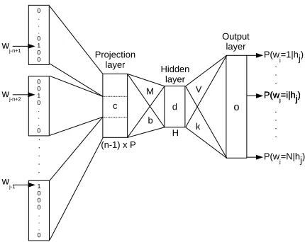
Figure 1: Neural network language model architecture.

in (Schwenk, 2007).

Figure 1 shows the architecture of a neural net-work language model. Each word in the vocabu-lary is represented by aNdimensional sparse vector where only the index of that word is 1 and the rest of the entries are 0. The input to the network is the concatenated discrete feature representations of n-1 previous words (history), in other words the indices of the history words. Each word is mapped to its continuous space representation using linear projec-tions. Basically discrete to continuous space map-ping is a look-up table withN xP entries whereN is the vocabulary size and P is the feature dimen-sion.i’th row of the table corresponds to the contin-uous space feature representation ofi’th word in the vocabulary. The continuous feature vectors of the history words are concatenated and the projection layer is performed. The hidden layer has H hidden units and it is followed by hyperbolic tangent non-linearity. The output layer has N targets followed by the softmax function. The output layer posterior probabilities,P(wj =i|hj), are the language model

probabilities of each word in the output vocabulary for a specific history,hj.

are as follows:

dj = tanh





(n−1)×_P

X

l=1

Mjlcl+bj



 ∀j= 1,· · ·, H

oi = H

X

j=1

Vijdj +ki∀i= 1,· · ·, N

pi =

exp(oi)

PN

r=1exp(or)

=P(wj =i|hj)

wherebj and ki are the hidden and output layer

bi-ases respectively.

The computational complexity of this model is dominated by HxN multiplications at the output layer. Therefore, a shortlist containing only the most frequent words in the vocabulary is used as the out-put targets to reduce outout-put layer complexity. Since NNLM distribute the probability mass to only the target words, a background language model is used for smoothing. Smoothing is performed as described in (Schwenk, 2007). Standard back-propagation al-gorithm is used to train the model.

Note that NNLM architecture can also be con-sidered as a neural network with two hidden layers. The first one is a hidden layer with linear activations and the second one is a hidden layer with nonlin-ear activations. Through out the paper we refer the first layer the projection layer and the second layer the hidden layer. So the neural network architec-ture with a single hidden layer corresponds to the NNLM, and is also referred to as a single hidden layer NNLM to distinguish it from DNN LMs.

Deep neural network architecture has several lay-ers of nonlinearities. In DNN LM, we use the same architecture given in Figure 1 and make the network deeper by adding hidden layers followed by hyper-bolic tangent nonlinearities.

3 Experimental Set-up

3.1 Baseline ASR system

While investigating DNN LMs, we worked on the WSJ task used also in (Chen 2008) for model M lan-guage model. This set-up is suitable for our initial experiments since having a moderate size vocabu-lary minimizes the effect of using a shortlist at the output layer. It also allows us to compare our pre-liminary results with the state-of-the-art performing model M language model.

The language model training data consists of 900K sentences (23.5M words) from 1993 WSJ text with verbalized punctuation from the CSR-III Text corpus, and the vocabulary is the union of the training vocabulary and 20K-word closed test vo-cabulary from the first WSJ CSR corpus (Paul and Baker, 1992). For speech recognition experiments, a 3-gram modified Kneser-Ney smoothed language model is built from 900K sentences. This model is pruned to contain a total of 350K n-grams using entropy-based pruning (Stolcke, 1998) .

Acoustic models are trained on 50 hours

of Broadcast news data using IBM Attila

toolkit (Soltau et al., 2010). We trained a

cross-word quinphone system containing 2,176 context-dependent states and a total of 50,336 Gaussians.

From the verbalized punctuation data from the training and test portions of the WSJ CSR corpus, we randomly select 2,439 unique utterances (46,888 words) as our evaluation set. From the remaining verbalized punctuation data, we select 977 utter-ances (18,279 words) as our development set.

We generate lattices by decoding the develop-ment and test set utterances with the baseline acous-tic models and the pruned 3-gram language model. These lattices are rescored with an unpruned 4-gram

language model trained on the same data. After

rescoring, the baseline WER is obtained as 20.7% on the held-out set and 22.3% on the test set.

3.2 DNN language model set-up

weights are initialized randomly, as previous work has shown deeper networks have more impact on im-proved performance compared to pre-training (Seide et al., 2011).

The cross-entropy loss function is used during training, also referred to as fine-tuning or backprop-agation. For each epoch, all training data is random-ized. A set of 128 training instances, referred to as a mini-batch, is selected randomly without replace-ment and weight updates are made on this mini-batch. After one pass through the training data, loss is measured on a held-out set of 66.4K words and the learning rate is annealed (i.e. reduced) by a fac-tor of 2 if the held-out loss has not improved suf-ficiently over the previous iteration. Training stops after we have annealed the weights 5 times. This training recipe is similar to the recipe used in acous-tic modeling experiments (Sainath et al., 2012).

To evaluate our language models in speech recog-nition, we use lattice rescoring. The lattices gener-ated by the baseline acoustic and language models are rescored using 4-gram DNN language models. The acoustic weight for each model is chosen to op-timize word error rate on the development set.

4 Experimental Results

Our initial experiments are on a single hidden layer NNLM with 100 hidden units and 30 dimensional features. We chose this configuration for our ini-tial experiments because this models trains in one day of training on an 8-core CPU machine. How-ever, the performance of this model on both the held-out and test sets was worse than the baseline. We therefore increased the number of hidden units to 500, while keeping the 30-dimensional features. Training a single hidden layer NNLM with this con-figuration required approximately 3 days on an 8-core CPU machine. Adding additional hidden lay-ers does not have as much an impact in the train-ing time as increased units in the output layer. This is because the computational complexity of a DNN LM is dominated by the computation in the output layer. However, increasing the number of hidden units does impact the training time. We also experi-mented with different number of dimensions for the features, namely 30, 60 and 120. Note that these may not be the optimal model configurations for our

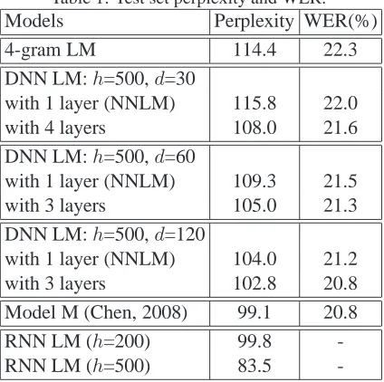
1 2 3 4

19 19.5 20 20.7

Number of hidden layers

Held−out set WER(%)

4−gram LM DNN LM: h=500, d=30 DNN LM: h=500, d=60 DNN LM: h=500, d=120

Figure 2: Held-out set WERs after rescoring ASR lattices with 4-gram baseline language model and 4-gram DNN language models containing up to 4 hidden layers.

set-up. Exploring several model configurations can be very expensive for DNN LMs, we chose these parameters arbitrarily based on our previous experi-ence with NNLMs.

Figure 2 shows held-out WER as a function of the number of hidden layers for 4-gram DNN LMs with different feature dimensions. The same number of hidden units is used for each layer. WERs are ob-tained after rescoring ASR lattices with the DNN language models only. We did not interpolate DNN LMs with the 4-gram baseline language model while exploring the effect of additional layers on DNN LMs. The performance of the 4-gram baseline lan-guage model after rescoring (20.7%) is shown with a dashed line.hdenotes the number of hidden units for each layer and ddenotes the feature dimension at the projection layer. DNN LMs containing only a single hidden layer corresponds to the NNLM. Note that increasing the dimension of the features im-proves NNLM performance. The model with 30 di-mensional features has 20.3% WER, while increas-ing the feature dimension to 120 reduces the WER to 19.6%. Increasing the feature dimension also shifts the WER curves down for each model. More im-portantly, Figure 2 shows that using deeper networks helps to improve the performance. The 4-layer DNN LM with 500 hidden units and 30 dimensional

fea-tures (DNN LM: h = 500 and d = 30) reduces

the WER from 20.3% to 19.6%. For a DNN LM with 500 hidden units and 60 dimensional features

(DNN LM:h= 500andd= 60), the 3-layer model

hid-den units and 120 dimensional features (DNN LM: h = 500 and d = 120), the WER curve plateaus after the 3-layer model. For this model the WER reduces from 19.6% to 19.2%.

We evaluated models that performed best on the held-out set on the test set, measuring both perplex-ity and WER. The results are given in Table 1. Note that perplexity and WER for all the models were cal-culated using the model by itself, without

interpolat-ing with a baseline n-gram language model. DNN

LMs have lower perplexities than their single hid-den layer counterparts. The DNN language models for each configuration yield 0.2-0.4% absolute im-provements in WER over NNLMs. Our best result on the test set is obtained with a 3-layer DNN LM with 500 hidden units and 120 dimensional features. This model yields 0.4% absolute improvement in WER over the NNLM, and a total of 1.5% absolute improvement in WER over the baseline 4-gram lan-guage model.

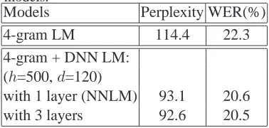
Table 1: Test set perplexity and WER.

Models Perplexity WER(%)

4-gram LM 114.4 22.3

DNN LM:h=500,d=30

with 1 layer (NNLM) 115.8 22.0

with 4 layers 108.0 21.6

DNN LM:h=500,d=60

with 1 layer (NNLM) 109.3 21.5

with 3 layers 105.0 21.3

DNN LM:h=500,d=120

with 1 layer (NNLM) 104.0 21.2

with 3 layers 102.8 20.8

Model M (Chen, 2008) 99.1 20.8

RNN LM (h=200) 99.8

-RNN LM (h=500) 83.5

-Table 1 shows that DNN LMs yield gains on top of NNLM. However, we need to compare deep net-works with shallow netnet-works (i.e. NNLM) with the same number of parameters in order to conclude that DNN LM is better than NNLM. Therefore, we trained different NNLM architectures with varying projection and hidden layer dimensions. All of these models have roughly the same number of parameters (8M) as our best DNN LM model, 3-layer DNN LM

with 500 hidden units and 120 dimensional features. The comparison of these models is given in Table 2. The best WER is obtained with DNN LM, showing that deep architectures help in language modeling.

Table 2: Test set perplexity and WER. The models have 8M parameters.

Models Perplexity WER(%)

NNLM:h=740,d=30 114.5 21.9

NNLM:h=680,d=60 108.3 21.3

NNLM:h=500,d=140 103.8 21.2

DNN LM:h=500,d=120

with 3 layers 102.8 20.8

We also compared our DNN LMs with a model M LM and a recurrent neural network LM (RNNLM) trained on the same data, considered to be cur-rent state-of-the-art techniques for language model-ing. Model M is a class-based exponential language model which has been shown to yield significant im-provements compared to conventional n-gram lan-guage models (Chen, 2008; Chen et al., 2009). Be-cause we used the same set-up as (Chen, 2008), model M perplexity and WER are reported directly in Table 1. Both the 3-layer DNN language model and model M achieve the same WER on the test set; however, the perplexity of model M is lower.

The RNNLM is the most similar model to DNN LMs because the RNNLM can be considered to have a deeper architecture thanks to its recurrent connec-tions. However, the RNNLM proposed in (Mikolov et al., 2010) has a different architecture at the in-put and outin-put layers than our DNN LMs. First, RNNLM does not have a projection layer. DNN LM hasN ×P parameters in the look-up table and

a weight matrix containing (n−1)×P ×H

a little effect compared to 10,000 ×H additional parameters introduced in RNNLM due to the use of the full vocabulary at the output layer.

We only compared DNN and RNN language models in terms of perplexity since we can not di-rectly use RNNLM in our lattice rescoring frame-work. We trained two models using the RNNLM toolkit1, one with 200 hidden units and one with 500 hidden units. In order to speed up training, we used 150 classes at the output layer as described in (Mikolov et al., 2011b). These models have 8M

and 21M parameters respectively. RNNLM with

200 hidden units has the same number of parameters with our best DNN LM model, 3-layer DNN LM with 500 hidden units and 120 dimensional features. The results are given in Table 1. This model results in a lower perplexity than DNN LMs. RNNLM with 500 hidden units results in the best perplexity in Ta-ble 1 but it has much more parameters than DNN LMs. Note that, RNNLM uses the full history and DNN LM uses only the 3-word context as the his-tory. Therefore, increasing the n-gram context can help to improve the performance for DNN LMs.

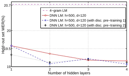
We also tested the performance of NNLM and DNN LM with 500 hidden units and 120-dimensional features after linearly interpolating with the 4-gram baseline language model. The interpola-tion weights were chosen to minimize the perplexity on the held-out set. The results are given Table 3. After linear interpolation with the 4-gram baseline language model, both the perplexity and WER im-prove for NNLM and DNN LM. However, the gain with 3-layer DNN LM on top of NNLM diminishes.

Table 3: Test set perplexity and WER with the interpo-lated models.

Models Perplexity WER(%)

4-gram LM 114.4 22.3

4-gram + DNN LM: (h=500,d=120)

with 1 layer (NNLM) 93.1 20.6

with 3 layers 92.6 20.5

One problem with deep neural networks, espe-cially those with more than 2 or 3 hidden lay-ers, is that training can easily get stuck in local

1_{http://www.fit.vutbr.cz/}

∼imikolov/rnnlm/

minima, resulting in poor solutions. Therefore,

it may be important to apply pre-training (Hinton et al., 2006) instead of randomly initializing the weights. In this paper we investigate discrimina-tive pre-training for DNN LMs. Past work in acous-tic modeling has shown that performing discrimina-tive pre-training followed by fine-tuning allows for fewer iterations of fine-tuning and better model per-formance than generative pre-training followed by fine-tuning (Seide et al., 2011).

In discriminative pre-training, a NNLM (one pro-jection layer, one hidden layer and one output layer) is trained using the cross-entropy criterion. Af-ter one pass through the training data, the output layer weights are discarded and replaced by another randomly initialized hidden layer and output layer. The initially trained projection and hidden layers are held constant, and discriminative pre-training is performed on the new hidden and output layers. This discriminative training is performed greedy and layer-wise like generative pre-training.

After pre-training the weights for each layer, we explored two different training (fine-tuning) scenar-ios. In the first one, we initialized all the lay-ers, including the output layer, with the pre-trained weights. In the second one, we initialized all the layers, except the output layer, with the pre-trained weights. The output layer weights are initialized randomly. After initializing the weights for each layer, we applied our standard training recipe.

Figure 3 and Figure 4 show the held-out WER as a function of the number of hidden layers for the case of no pre-training and the two discriminative pre-training scenarios described above using models with 60- and 120-dimensional features. In the fig-ures, pre-training 1 refers to the first scenario and pre-training 2 refers to the second scenario. As seen in the figure, pre-training did not give consistent gains for models with different number of hidden layers. We need to investigate discriminative pre-training and other pre-pre-training strategies further for DNN LMs.

5 Related Work

1 2 3 4 19

19.5 20 20.7

Number of hidden layers

Held−out set WER(%)

4−gram LM DNN LM: h=500, d=60

DNN LM: h=500, d=60 (with disc. pre−training 1) DNN LM: h=500, d=60 (with disc. pre−training 2)

Figure 3: Effect of discriminative pre-training for DNN LM:h=500,d=60.

1 2 3 4

19 19.5 20 20.7

Number of hidden layers

Held−out set WER(%)

4−gram LM DNN LM: h=500, d=120

DNN LM: h=500, d=120 (with disc. pre−training 1) DNN LM: h=500, d=120 (with disc. pre−training 2)

Figure 4: Effect of discriminative pre-training for DNN LM:h=500,d=120.

words together with the probability function of word

sequences. This NNLM approach is extended to

large vocabulary speech recognition in (Schwenk and Gauvain, 2005; Schwenk, 2007) with some speed-up techniques for training and rescoring. Since the input structure of NNLM allows for using larger contexts with a little complexity, NNLM was also investigated in syntactic-based language mod-eling to efficiently use long distance syntactic infor-mation (Emami, 2006; Kuo et al., 2009). Significant perplexity and WER improvements over smoothed n-gram language models were reported with these efforts.

Performance improvement of NNLMs comes at

the cost of model complexity. Determining the

output layer of NNLMs poses a challenge mainly

attributed to the computational complexity.

Us-ing a shortlist containUs-ing the most frequent several thousands of words at the output layer was pro-posed (Schwenk, 2007), however, the number of hidden units is still a restriction. Hierarchical de-composition of conditional probabilities has been proposed to speed-up NNLM training. This decom-position is performed by partitioning output vocab-ulary words into classes or by structuring the output layer to multiple levels (Morin and Bengio, 2005; Mnih and Hinton, 2008; Son Le et al., 2011). These approaches provided significant speed-ups in train-ing and make the traintrain-ing of NNLM with full vo-cabularies computationally feasible.

In the NNLM architecture proposed in (Bengio et al., 2003), a feed-forward neural network with a single hidden layer was used to calculate the lan-guage model probabilities. Recently, a recurrent

neural network architecture was proposed for lan-guage modelling (Mikolov et al., 2010). In con-trast to the fixed content in feed-forward NNLM, re-current connections allow the model to use arbitrar-ily long histories. Using classes at the output layer was also investigated for RNNLM to speed-up the training (Mikolov et al., 2011b). It has been shown that significant gains can be obtained on top of a very good state-of-the-art system after scaling up RNNLMs in terms of data and model sizes (Mikolov et al., 2011a).

There has been increasing interest in using neu-ral networks also for acoustic modeling. Hidden Markov Models (HMMs), with state output distri-butions given by Gaussian Mixture Models (GMMs) have been the most popular methodology for acous-tic modeling in speech recognition for the past 30 years. Recently, deep neural networks (DNNs) (Hin-ton et al., 2006) have been explored as an alternative to GMMs to model state output distributions. DNNs were first explored on a small vocabulary phonetic recognition task, showing a 5% relative improve-ment over a state-of-the-art GMM/HMM baseline system (Dahl et al., 2010). Recently, DNNs have been extended to large vocabulary tasks, showing a 10% relative improvement over a GMM/HMM sys-tem on an English Broadcast News task (Sainath et al., 2012), and a 25% relative improvement on a con-versational telephony task (Seide et al., 2011).

not been investigated before for language modeling. RNNLMs are the closest to our work since recurrent connections can be considered as a deep architecture where weights are shared across hidden layers.

6 Conclusion and Future Work

In this paper we investigated training language

mod-els with deep neural networks. We followed the

feed-forward neural network architecture and made the network deeper with the addition of several lay-ers of nonlinearities. Our preliminary experiments on WSJ data showed that deeper networks can also

be useful for language modeling. We also

com-pared shallow networks with deep networks with the same number of parameters. The best WER was obtained with DNN LM, showing that deep

archi-tectures help in language modeling. One

impor-tant observation in our experiments is that perplex-ity and WER improvements are more pronounced with the increased projection layer dimension in NNLM than the increased number of hidden layers in DNN LM. Therefore, it is important to investigate deep architectures with larger projection layer di-mensions to see if deep architectures are still useful. We also investigated discriminative pre-training for DNN LMs, however, we do not see consistent gains. Different pre-training strategies, including genera-tive methods, need to be investigated for language modeling.

Since language modeling with DNNs has not been investigated before, there is no recipe for building DNN LMs. Future work will focus on elaborating training strategies for DNN LMs, including investi-gating deep architectures with different number of hidden units and pre-training strategies specific for language modeling. Our results are preliminary but they are encouraging for using DNNs in language modeling.

Since RNNLM is the most similar in architecture to our DNN LMs, it is important to compare these two models also in terms of WER. For a fair com-parison, the models should have similar n-gram con-texts, suggesting a longer context for DNN LMs. The increased depth of the neural network typi-cally allows learning more patterns from the input data. Therefore, deeper networks can allow for bet-ter modeling of longer contexts.

The goal of this study was to analyze the behav-ior of DNN LMs. After finding the right training recipe for DNN LMs in WSJ task, we are going to compare DNN LMs with other language modeling approaches in a state-of-the-art ASR system where the language models are trained with larger amounts of data. Training DNN LMs with larger amounts of data can be computationally expensive, however, classing the output layer as described in (Mikolov et al., 2011b; Son Le et al., 2011) may help to speed up training.

References

Yoshua Bengio, Rejean Ducharme, Pascal Vincent, and Christian Jauvin. 2003. A neural probabilistic lan-guage model. Journal of Machine Learning Research, 3:1137–1155.

Yoshua Bengio. 2007. Learning Deep Architectures for AI. Technical report, Universit e de Montreal. S. F. Chen and J. Goodman. 1999. An empirical study of

smoothing techniques for language modeling. Com-puter Speech and Language, 13(4).

Stanley F. Chen, Lidia Mangu, Bhuvana Ramabhadran, Ruhi Sarikaya, and Abhinav Sethy. 2009. Scaling shrinkage-based language models. In Proc. ASRU 2009, pages 299–304, Merano, Italy, December. Stanley F. Chen. 2008. Performance prediction for

expo-nential language models. Technical Report RC 24671, IBM Research Division.

George E. Dahl, Marc’Aurelio Ranzato, Abdel rah-man Mohamed, and Geoffrey E. Hinton. 2010. Phone Recognition with the Mean-Covariance Re-stricted Boltzmann Machine. In Proc. NIPS.

Ahmad Emami. 2006. A neural syntactic language model. Ph.D. thesis, Johns Hopkins University, Bal-timore, MD, USA.

Geoffrey E. Hinton, Simon Osindero, and Yee-Whye Teh. 2006. A Fast Learning Algorithm for Deep Belief Nets. Neural Computation, 18:1527–1554.

H-K. J. Kuo, L. Mangu, A. Emami, I. Zitouni, and Y-S. Lee. 2009. Syntactic features for Arabic speech recognition. In Proc. ASRU 2009, pages 327 – 332, Merano, Italy.

Tomas Mikolov, Martin Karafiat, Lukas Burget, Jan Cer-nocky, and Sanjeev Khudanpur. 2010. Recurrent neu-ral network based language model. In Proc. INTER-SPEECH 2010, pages 1045–1048.

Tomas Mikolov, Stefan Kombrink, Lukas Burget, Jan Cernocky, and Sanjeev Khudanpur. 2011b. Exten-sions of recurrent neural network language model. In Proc. ICASSP 2011, pages 5528–5531.

Andriy Mnih and Geoffrey Hinton. 2008. A scalable hi-erarchical distributed language model. In Proc. NIPS. Abdel-rahman Mohamed, George E. Dahl, and Geoffrey Hinton. 2009. Deep belief networks for phone recog-nition. In Proc. NIPS Workshop on Deep Learning for Speech Recognition and Related Applications. Frederic Morin and Yoshua Bengio. 2005. Hierarchical

probabilistic neural network language model. In Proc. AISTATS05, pages 246–252.

Douglas B. Paul and Janet M. Baker. 1992. The de-sign for the wall street journal-based csr corpus. In Proc. DARPA Speech and Natural Language Work-shop, page 357362.

Tara N. Sainath, Brian Kingsbury, and Bhuvana Ramab-hadran. 2012. Improvements in Using Deep Belief Networks for Large Vocabulary Continuous Speech Recognition. Technical report, IBM, Speech and Lan-guage Algorithms Group.

Ruhi Sarikaya, Mohamed Afify, and Brian Kingsbury. 2009. Tied-mixture language modeling in continuous space. In HLT-NAACL, pages 459–467.

Holger Schwenk and Jean-Luc Gauvain. 2005. Training neural network language models on very large corpora. In Proc. HLT-EMNLP 2005, pages 201–208.

Holger Schwenk. 2007. Continuous space language models. Comput. Speech Lang., 21(3):492–518, July. Frank Seide, Gang Li, Xie Chen, and Dong Yu. 2011.

Feature Engineering in Context-Dependent Deep Neu-ral Networks for Conversational Speech Transcription. In Proc. ASRU.

Hagen Soltau, George. Saon, and Brian Kingsbury. 2010. The IBM Attila speech recognition toolkit. In Proc. IEEE Workshop on Spoken Language Technology, pages 97–102.

Hai Son Le, Ilya Oparin, Alexandre Allauzen, Jean-Luc Gauvain, and Francois Yvon. 2011. Structured out-put layer neural network language model. In Pro-ceedings of IEEE International Conference on Acous-tic, Speech and Signal Processing, pages 5524–5527, Prague, Czech Republic.