Optimal design and strategy for the SolUTra

University of Twente

EEMCS / Electrical Engineering

Control Engineering

Optimal design and strategy for the SolUTra

Ceriel Mocking

MSc Report

Supervisors:

prof.dr.ir. J. van Amerongen dr.ir. P.C. Breedveld dr.ir. J.F Broenink

January 2006

Abstract

In the past 2 years, a multidisciplinary team of students of the University of Twente has been designing and building the SolUTra, a solar powered racing car. The SolUTra participated in the 2005 World Solar Challenge, a 3000 km race, solely for cars powered by solar energy, through the outback of Australia.

Such a project not only provides the obvious mechanical and electric challenges to a Solar Team, it also involves finding a way to efficiently use all available energy, while trying to be the first at the finish line.

This report treats the design of a strategy development program (PALLAS), which is to be used to determine an optimal racing strategy for the SolUTra solar car during the race. The report also provides an overview of the proceedings of the race in Australia and the use of PALLAS during the race.

PALLAS proved to be of great value, as it discovered erroneous car tunings in time, was able to develop optimal racing strategies and to determine the consequences of strategic decisions.

However, PALLAS suffers from model inaccuracies due to lack of testing and inaccurate measure-ment equipmeasure-ment, which decreases the reliability of the developed strategies. The inaccuracy of the mea-surement equipment also decreases the ability to monitor and check the strategy that is maintained.

Preface

In the last 2 years, the whole of my studies was directed at a single goal; Strategy & design for the SolUTra solar car. 13 other determined students were also working hard as well, having just one thing in mind: Participating in the World Solar Challenge with our own solar car.

After the initial phase of setting up a team, we found our big supporters: The University of Twente bought our motor, Raedthuys bought the solar cells and THALES was eager to help us at everything we needed help for. And a lot of other companies supported us as well. Backed by the sponsors, the UT and several tutors, we were able to design and build the SolUTra! And suddenly we found ourselves in Australia...

But for this particular project, I want to thank Prof. van Amerongen, dr. Broenink and dr. Breedveld for providing me the opportunity to graduate on this ambitious project, which is so unlike any other project of the Control Engineering chair. Perhaps, it’s only the first of a number of similar projects...

Thanks go as well to Valer Pop, MSc, who introduced me to battery theory and SOC measurements. His input was right on time. Valer Pop, MSc, who was the first to instruct me in battery theory and SOC measurements. His input was right on time.

And, yes, I even like to thank my rival strategists in the Nuon Solar Team and the Aurora Solar Team, Eric Trottemant and dr. Peter Pudney, who, although it is a cliché, both showed me the way I had to tread, in order to become a solar team strategist.

Furthermore, I like to thank my loving family, who were always ready to support me, whenever I needed. And Mira? Sorry that I left you waiting for such a long time, while writing this report...

I like to say one last word to my fellow team members: "Yeah, mates! We did it!"

Ceriel Mocking,

Definitions

Air mass index The air mass index is a measure for the thickness of the layer of air the sun rays have to

pass through, before reaching the earth’s surface.

Altitude angle The angle of the sun above the horizon;

Angle of Attack In literature concerning aerodynamics, Angle of Attack is defined as the pitch angle of

the air flow relative to the object. In this project, angle of attack is defined as the yaw angle of the car relative to the air flow.

(Battery) equilibrium curve When in equilibrium (after a rest period of at least 2 hours) a battery goes

in to equilibrium state, in which the output voltage is directly related to the battery SOC. The equilibrium curve is measured by discharging or charging the battery completely in a minimal time of 20 hours (0.05 CmA), such that the battery does not leave the equilibrium state.

Battery SOC Battery State-of-Charge or Accu State-of-Charge. The battery SOC is the amount of

charge left in the battery. The battery SOC can be measured both in kWh and in a percentage;

BIPM Bureau International des Poids et Mesures. Part of the CIPM;

BVP Boundary Value Problem;

(Solar) Car model The car model calculates the input and output power of the car, the battery charge,

the distance traveled as a function of car speed. It takes account of night stops, media stops, speed limits etc.;led as a function of car speed. It takes account of night stops, media stops, speed limits etc.;

CIPM Comité International des Poids et Mesures;

Constant average car speed strategy or similar. A strategy in whichv(t) = v0. An extension to this

strategy is using a number of stages, each having its own optimal average speed. e.g. v(t) = vi

for the i-th stage. A racing strategy developed by PALLAS generally has the form of a vector of constant car speeds;

CmA or simply ’C’: a battery charge or discharge current rate. A current rate of precisely 1.0 CmA will

cause a fully charged battery to discharge completely in precisely 1 hour;

Cost Criterion The objective of optimization is to minimize the cost criterion. Synonyms: Objective

function, optimization criterion;

Diffuse light Insolation Sunlight received indirectly as a result of scattering due to clouds, fog, haze,

vi

Direct Beam Insolation Direct solar irradiance; unreflected solar energy;

Drag Air friction;

EWMA chart The ’Exponentially Weighted Moving Average’ is a weighted moving average, for which

events in the past are exponentially weighted. Basically a 1st order low-pass filter, used in Stochas-tic Process Control;

GUIDE ’Graphical User Interface Development Environment’. A Matlab tool for designing and

build-ing user interfaces;

Insolation The amount of solar radiance on a surface;

Irradiance Similar to ’insolation’;

Media stop A 30 min stop, during which the press is allowed to interview the solar teams;

MPPT ’Maximum Power Point Tracker’, used to keep the solar array functioning optimally;

Night stop every day, the Solar Team is compelled to stop at 5 p.m. and make camp at the side of the

road. The Solar Team may continue driving at 8 a.m. next morning. When not racing, the solar array is always pointed to the sun, in order to charge the batteries;

ODE Ordinary Differential Equation;

OP Optimization problem;

Optimization (input) parameter An optimization method varies this parameter to find the minimum

of the cost criterion;

PALLAS ’PALLAS’ is the name of the Strategy Development Program. ’Pallas’ originates from the

goddess Pallas Athena, who is the classical Greek personification of Strategy & Tactics and the patroness of generals and strategists;

Projection With projecting or forecasting, the prediction of future events is meant. In this particular

case, it means the use of regression to foretell the results of ’staying on course’;

Regenerative braking Braking by using the motor as an electric generator, such that part of the kinetic

energy of the car is transformed in electric energy that can be stored in the batteries;

Road model The model of the racing track, consisting of slope, road conditions, weather expectations,

GPS positions, speed limits, etc.;

SDP ’SDP’is the abbreviation of ’Strategy Development Program’;

SolUTra The name of the Solar Car;

STUNT Solar Team Universal Network Technology: the software associated to the STUT;

Symbols

α Slope angle

A Effective area of Solar array (panel)

Ad Effective drag area (top surface of SolUTra)

CB Cloud Brightness

crr Roll friction coefficient

cr1 Static Roll friction coefficient

cr2 Dynamic Roll friction coefficient

CW Drag coefficient

δ Angle between car vector and air speed vector

ηec Effectiveness of charging the batteries before 8 a.m. and after 5 p.m.

ηrb Effectiveness regenerative braking

ηmppt MPPT efficiency

ηm Motor efficiency

ηp Solar array (panel) efficiency

EOT ’Equation of Time’

γ Perpendicular angle of sun; the angle between the horizon and the sun

g Gravitational constant (g∼= 9.81)

g(Q(t)) Battery safety limit function

J Cost Criterion

lat latitude

long longitude

m Air mass index

mc Mass of Solar Car

n Number of wheels

φ Car Direction

Ψlocal Local reference frame

ψlocal Local meridian

Pin Input power

Pout Output power (Power consumption)

P0 Constant Output power factor

Q(t) Battery State-of-Charge (SOC)

Q0 Battery State-of-Charge Initial value

viii

Q+

Upper battery safety limit

Q−

Lower battery safety limit

ρ Air density

SC Sun Coverage

θ Wind Direction

te End of simulation time

~vef f Air speed vector

~vcaror~v Car speed vector

~vwind Wind speed vector

~

w Vector of weights

x(t) Traveled distance; distance from start

x0 Traveled distance, initial value

Contents

1 Introduction & Problem Definition 1

1.1 Introduction . . . 1

1.2 Problem definition . . . 2

1.3 STUNT . . . 4

1.4 PALLAS . . . 4

1.5 Report outline . . . 5

2 Solar Car Model 7 2.1 Introduction . . . 7

2.2 Power Consumption . . . 9

2.3 Insolation . . . 14

2.4 Batteries . . . 18

2.5 Testing the Solar Car Model . . . 21

3 Strategy Optimization 25 3.1 Introduction & Optimization Problem . . . 25

3.2 Optimization methods . . . 28

3.3 Optimization in PALLAS . . . 31

4 Monitoring 35 4.1 Introduction . . . 35

4.2 Model Accuracy . . . 35

4.3 Monitoring Measurements . . . 38

4.4 Statistical Process Control . . . 41

4.5 Projection . . . 44

4.6 Application & Implementation . . . 45

5 Software Realization 47 5.1 Introduction . . . 47

5.2 Optimization . . . 48

5.3 Monitoring . . . 53

5.4 Using PALLAS . . . 55

6 Testing & Application 57 6.1 Introduction . . . 57

6.2 Identifying & Testing the SolUTra Model . . . 57

x CONTENTS

6.4 The Race . . . 67

7 Conclusions & Recommendations 79 7.1 Conclusions . . . 79

7.2 Recommendations . . . 80

A Symbolic Optimization 83 A.1 Minimum Principle (Pontryagin) . . . 83

A.2 Model equations . . . 84

A.3 Solving the optimal Strategy Problem using Pontryagin . . . 84

B Numerical Optimization methods 87 B.1 Convexity . . . 87

B.2 Numerical Optimization . . . 88

B.3 Global Optimization . . . 92

C Controlling battery current instead of Car speed 93 C.1 Introduction . . . 93

C.2 Car model - advanced . . . 93

C.3 Pontryagin - again . . . 94

C.4 Results: points of interests . . . 95

C.5 Conclusions . . . 96

D Programming PALLAS in Matlab 97 D.1 Introduction . . . 97

D.2 Matlab GUIDE . . . 97

D.3 PALLAS GUI . . . 101

D.4 PALLAS program . . . 105

E STUNT Database 113 E.1 About the Database . . . 113

E.2 Design . . . 113

E.3 Telemetry system: the weather forecast . . . 114

F Detailed recommendations 115 F.1 Improving the Car Model . . . 115

F.2 Sensors . . . 116

F.3 PALLAS programming . . . 118

G 2005 Panasonic World Solar Challenge 119

Chapter 1

Introduction & Problem Definition

1.1

Introduction

1.1.1 Solar Team University of Twente & the World Solar Challenge

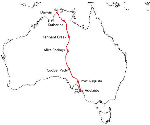
The Team The Dutch Solar Team University of Twente (officially ’Raedthuys Solar Team’) is formed in May 2003 with a single goal: participating in the 2005 World Solar Challenge, a 3000 km race from Darwin to Adelaide through the Australian outback (Fig. 1.1) for cars solely powered by solar energy.

Katharine Darwin

Tennant Creek

Alice Springs

Coober Pedy

Port Augusta

Adelaide

Figure 1.1: World Solar Challenge race track (Stuart Highway).

2 1. INTRODUCTION & PROBLEM DEFINITION

The WSC The World Solar Challenge is a bi-annual event, that is held for the eighth time in 2005. Originally, it was a race for solar powered cars only (divided in ’production’ class for 2 or more persons and larger solar arrays, and an ’open’ class, in which a car is allowed to carry only 1 person, but has more restrictions in battery and solar array size). Nowadays, also a Greenfleet-class (using renewable energy in general) and a Solar bicycle class (bicycling aided by solar power) are part of the World Solar Challenge.

The Solar Team will participate in the ’open’ class race, which will take the team through the Aus-tralian Outback following the Stuart Highway.

The goal of the WSC is mainly to promote the use of renewable energy. More information can be found on the WSC websitewww.wsc.org.au.

1.1.2 The SolUTra

A solar car is fundamentally built for efficiency and speed. Driver comfort, good looks and affordability are secondary goals.

Most solar cars are of sleek design to minimize drag, with a large solar array on top to collect as much solar power as possible. The SolUTra is not different. She has three wheels, as this results in less roll friction, with 2 wheels in front and one in the rear, which is also the driving wheel. The electro motor used is an ’in-wheel’ motor, which means that it is directly attached to the wheel. In this way, there is no need for transmission anymore, increasing the efficiency of driving.

The design of the solar car consists of 3 main fields of interest: Mechanics, Electronics and Telemetry. Mechanically, the car is designed for minimal drag and roll friction, while electronically, the car is optimized for energy efficiency. Telemetry deals with measuring relevant quantities and transporting and storing the measurement data.

Electronics The SolUTra contains a Worly Li-Polymer battery pack, that is charged via the AsGe-solar array. 5 DriveTek Maximum Power Point Trackers ensure that the solar array delivers maximum power. The battery supplies energy to an NGM brushless DC electro motor (combination of an NGM AC motor and Tritium Gold DC/AC motorcontroller).

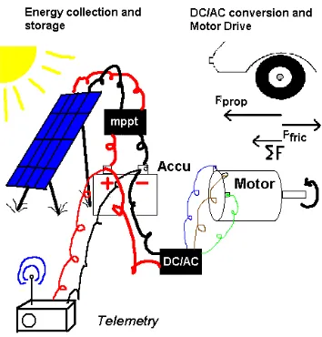
The battery also supplies power to the telemetry system, consisting of various sensors and a WLAN system for communications with the chase car. See Fig. 1.2 for an overview of the basic solar car parts.

Mechanics Mechanical challenges in the SolUTra project consisted of designing a chassis of which the drag is to be minimized, wheel spats that turn with the wheel, the suspension of the wheels that had to fit in the chassis and a steering system for a car in which a steering wheel simply does not fit.

Telemetry Measurement data from the SolUTra is transported via a WLAN to the chase car. The chase car contains some sensors as well, like a GPS and a weather station. All measurement data is stored in a database for analysis or other uses

1.2

Problem definition

The main challenge of the STUT is to find a way to be the first team to arrive at the finish line, with limited battery capacity and being compelled to using solar energy only.

To do this, the solar team has to:

PROBLEM DEFINITION 3

Figure 1.2: Basic parts of the SolUTra Solar Car

2. drive as fast as possible with the available energy.

This report describes the tackling of the problem of finding a racing strategy that, when followed, would bring the SolUTra to Adelaide as fast as possible.

1.2.1 Project Goal

The goal of this graduation project is to develop an optimal racing strategy for the SolUTra solar car, which minimizes the time needed for the SolUTra to reach the finish line. Although the SolUTra is able to reach a car speed of over 100km_{/h, she may not have enough energy available to keep top speed for the}

total distance of the race.

Now, the problem can be regarded as a time-optimal control problem. An optimal car speed has to be found, that controls the balance between input and output power such, that racing time is minimized. The batteries act as an energy buffer. As long as the batteries do contain energy, the car speed can be chosen freely. Otherwise, the car speed is constrained by the input power. It is therefore imperative, that the batteries are never completely emptied (except at the finish line).

1.2.2 Balancing battery State-of-Charge

The car speed controls the balance between input power and output power and therefore the available energy in the batteries, which, in turn, constrains the car speed. Thus, the car speed has to be chosen such, that the SolUTra reaches the finish line as soon as possible, while satisfying the battery condition of always having energy available in the battery.

The effect of a certain car speed on the battery State-of-Charge (SOC) can only be estimated, when it can be predicted how much energy will be used for driving and how much energy will be collected.

4 1. INTRODUCTION & PROBLEM DEFINITION

There are a lot of factors that will influence the battery SOC. All these factors have to be measured in some way in order to use them for power consumption predictions. Measurement and prediction calculations can be automated in order to be able to provide information to the team as soon as possible, as this information is to be used for planning. In this way, automation provides a way to calculate the best way to use the available energy.

In other words, automation provides a way to design an optimal racing strategy, which brings the solar car to the finish line as soon as possible.

1.2.3 Strategy Development Program

To automate the determination of an optimal racing strategy, a Strategy Development Program (SDP) is to be designed. The task of the SDP is to develop a racing strategy, which is basically a car speed setpoint to the car driver. The SDP can use all available data to perform its task, while being able to react at changing situations.

The SDP has to calculate an optimal car speed guideline. The SDP must also be able to calculate a new strategy, if the one adopted becomes useless. This happens when, for example, the car falls behind schedule. As the chances of being thrown off-schedule by traffic lights, flat tyres and such, are so big that it is virtually certain that this will happen, the SDP must be sufficiently robust to deal with such stress situations. And it has to do this quickly, as it is advisable to follow the optimal strategy as much as possible. This introduces a design requirement of being able to calculate the optimal strategy in mere minutes.

On the other hand, a very accurate car model is desired for accurate simulation and optimization and the SDP has to be provided with sufficient data and reliable predictions about the racing track in order to be able to develop a feasible strategy. However, the original plan of using adaptive modeling for improving the car model during tests had to be abandoned due to lack of time, so a static model has to be used.

1.3

STUNT

The Telemetry system is managed by the STUNT network, the ’Solar Team Universal Network Tech-nology’ network, which has been built by Vincent Groenhuis, the Solar Team Telemetrist. This network collects all sensor readings and performs a fast scan of the data for alarming situations.

The network contains a MySQL database (the STUNT Database), which stores virtually everything regarding the SolUTra project. Apart from the car sensor measurements, the STUNT Database holds an electronic logbook, a list of static data (such as GPS positions, altitude, inclination, etc) regarding various racing tracks, weather forecasts etc. The SDP is only allowed to make use of the STUNT Database. The communication interface between the SDP and the STUNT Database is designed and built by Vincent Groenhuis.

1.4

PALLAS

REPORT OUTLINE 5

1.5

Report outline

The report starts with the design and the various aspects of the solar car model. Chapter 3 explains the optimization of the racing strategy, while chapter 4 shows how PALLAS checks whether the solar car is on schedule or not.

Chapter 5 treats the realization of PALLAS and chapter 6 shows how PALLAS is used during the World Solar Challenge race.

One word of advice

Chapter 2

Solar Car Model

2.1

Introduction

2.1.1 Model requirements

In order to calculate the impact of choosing a car speed on the battery SOC, a model has to be designed of the solar car. This model has to approximate input power (Pin) and output power (Pout), while driving

an approximation of the racing track. The model must

• be able to estimate the amount of solar irradiance during the day, in order to calculate the input power;

• be able to calculate the power delivered to the motor and the power dissipated in other electronic systems;

• be able to handle various WSC regulations (media stops etc.);

• be simple enough, such that optimization does not take more than a few minutes;

• include a cost criterion that calculates the ’fitness’ of a strategy.

The relevant model outputs are the distance traveled and the battery SOC as functions of time, which basically describe a racing strategy, together with the optimal car speedv∗

car(t).

2.1.2 Model layout

The general layout of the car model is shown in fig. 2.1. The submodels of the model are:

Sun_Model This submodel calculates the perpendicular irradiance of the sun and the angle of the sun

above horizon as a function of time and location;

Road_Model The road submodel supplies the external circumstances, such as wind, slope, GPS position

etc. These circumstances depend on the location of the SolUTra in Australia;

Speed_Setpoint The speed setpoint submodel supplies the car speed setpoint vcar(t) to the Solar car

submodel. It takes account of media stops, overnight stops etc.;

Solarcar_Model The solar car submodel uses the data from the Road and solar models and the Speed

8 2. SOLAR CAR MODEL Road_Model .txt Road_Model Sun_Model Criterion SOC x Criterion Speed_SP Speed_SetPoint SolarCar_Model road sun v_car x SOC SolarCar_Model Isol γ

(Sun Coverage, GPS position, Wind, slope etc.)

Vcar

Figure 2.1: The 20-Sim model that is used for optimization.

Criterion The Criterion submodel calculates the optimization criterionJ.

The Solar Car submodel is more extensively shown in Fig. 2.2. It can be seen that a distinction is made between input power calculations and output power calculations.

Insolation equations road sun γ Isol SC CB Vwind etc. Power Consumption road sun γ Isol SC CB Vwind etc. Vcar +

- Pout

Pin

Battery dQ(t)

= Pin - Pout dt

Figure 2.2: The design of the Solar Car submodel. The calculations made in the Solar Car submodel are devided in equations calculating the insolation power Pin and the power consumption Pout. The

difference between input and output power is buffered in the batteries.

2.1.3 Chapter outline

This chapter is dedicated to the implementation of the Sun submodel and the Solar car submodel: The chapter starts with explaining the aspects of the solar car model regarding the power consumption and subsequently, the equations which calculate the insolationare treated. In section 2.4, the battery, which buffers the difference between input and output power, and its characteristics are treated.

POWER CONSUMPTION 9

The chapter on solar car model design finishes with an overview and characterization of the solar car model and its parameters.

2.2

Power Consumption

The mechanical IPM and the bond graph of the solar car is shown in Fig. 2.3(a).

Fslope Froll Fdrag

Fmotor

Vcar

α

(a) Mechanical IPM

TF Wheel

I Car

R Roll

1 MSeGravity _Slope

Wind MR

Drag motor_current MSe

Motor

(b) Mechanical bond graph

Figure 2.3: The IPM and the corresponding bond graph of the mechanical aspect of the solar car.

The net force acting on the solar car is:

X

F =Fmotor−Fdrag−Froll−Fslope (2.1)

When considering the fact that the car speed is assumed to vary little over time. Dynamical effects regardingvcarare therefore relatively small, when compared to the large distance over which the race will

be simulated. So, simulation and optimization time can be greatly reduced by assuming thatP

F = 0

in eq. 2.1.

This assumption neglects the energy lost to acceleration of the car. The car motor, however, may be used as a generator when decelerating. In that way, some of the energy used for accelerating the car can be regained (’regenerative braking’). Energy lost to inefficiency in regenerative braking is neglected.

An important result of this assumption is, that the car speed can be directly chosen, such that the solar car inertia element in the bond graph of Fig. 2.3(b) becomes non-causal. This leaves only ’SolUTra’s position (distance from Darwin) and battery SOC as car states. The output power can then be directly calculated as a function of the car speed.

Outline

This Output Power section explains the implementation of the friction forces and the influence of slopes on the SolUTra. It also briefly treats the electro motor used to drive the SolUTra.

2.2.1 Drag

10 2. SOLAR CAR MODEL

(~vcar−~vwind).

The Drag ForceFdrag acting on the car, caused by air flow and car speed, is defined by:

Fdrag =c(δ)·~v2=

1

2ρCD(δ)Ad·~v

2

(2.2)

in whichCW(δ) = CD(δ)Advaries with the angle of attackδof the air flow and the top surfaceAdof

the car (fig. 2.5(a)).

Effective air flow

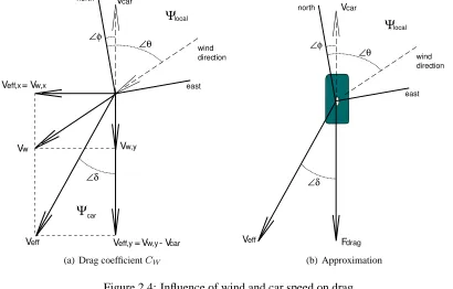
The effective air velocityvef f~ is determined by car speed vector~vcarand inbound wind vector~vwind. The

relation between these velocities is shown in fig. 2.4(a). This figure shows the direction (and magnitude) of the car velocity and wind velocity in the local reference frame (Ψlocal), which defines normal compass

directions. In order to calculate the effective air velocity:

Veff,x = Vw,x

Veff,y = Vw,y - Vcar

Veff Ψ_car Vw,y Vw Ψlocal Vcar wind direction ∠θ ∠φ ∠δ north east

(a) Drag coefficientCW

Fdrag Veff ∠δ Ψlocal Vcar wind direction ∠θ ∠φ north east (b) Approximation

Figure 2.4: Influence of wind and car speed on drag

vef f =

p

(v2

y +v

2

x) (2.3)

vef f,x = vwsin(θ−φ)

vef f,y = vcar+vwcos(θ−φ)

⇒v2ef f = v

2

car+ 2vcarvwcos(θ−φ) +vw2 (2.4)

And thus, for the drag force, the following applies:

Fdrag =

1

2ρCW(δ)·(v

2

car+ 2vcarvwcos(θ−φ) +v2w) (2.5)

POWER CONSUMPTION 11

Drag parameterCW

Fig. 2.5(a) shows the dependency ofCW ofδ, measured using a scale model of the solar car in a wind

tunnel (Putten, 2005).CW is approximated by eq. 2.6 (Ad=9 m2).

Cw

Cw Cw

−δ _δ

(0, 0) (0, 1)

(a) Air speed components

−100 −5 0 5 10

0.02 0.04 0.06 0.08 0.1

Drag coefficient C

w

δ

Cw

(b) Drag force

Figure 2.5:Cw as function of angle of attack)

CW(δ) = 9(−1.6·10−5δ2+ 8.9·10−3) (2.6)

For small values (less than app. 5°) ofδ,CW can be considered constant:

CW(δ) = 0.08 (2.7)

The wind tunnel test with the scale model is not followed by a test with the SolUTra herself. As the scale model is ideal (drag surface is very smooth), while the SolUTra itself has a lot of drag surface irregularities, the measured CW value is considered to be only a rough and optimistic estimation of

SolUTra’s drag coefficient. The dependency ofCW onδdoes apply to the scale model only.

Therefore, it is decided to use a constant value of the drag coefficient.

Air densityρ

The most widely used method of determining air density is the application of the CIPM-81/91 formula recommended by the ’Bureau International des Poids et Mesures’ (BIPM), which is a rather complicated equation. In an article without author (BIPM, n.d.) the CIPM-81/91 formula is given (eq. 2.8):

ρ= pMa

ZRT

h

1₋xv(1−

Mv

Ma

)i (2.8)

withpthe air pressure,T the temperature,xv the mole fraction of water vapour,Mathe molar mass of

dry air,Mvthe molar mass of water,Zthe compressibility factor and R the molar gas constant.

It is, however, simpler to start with the relation of eq. 2.9 and to use an approximation rather then use the complex relation of eq. 2.8.

ρ= p

R_·T (2.9)

12 2. SOLAR CAR MODEL

Pressure, Temperature and Humidity To correct for air humidity, (Shelquist, 2004) uses

ρ= p

R_·Tv

(2.10)

in whichTv is a virtual temperature, which depends on air humidity.Tvis approximated by:

Tv =

T 1₋c1E_p

(2.11)

E = c0·10

c1Tc

c2 +Tc (2.12)

in whichEis the saturation vapor pressure, which may be multiplied with the air humidity percentage to retrieve the actual vapor pressure. The virtual temperature will rise with increasing humidity (E), which causes the air density to drop.

Humidity has only a slight influence on air density compared to air temperature and air pressure. It will, however, increase with high temperatures and low air pressure. But for the purpose of simplicity, the influence of humidity is neglected. This still leaves the air density depending on temperature and pressure. Using 2nd-order Taylor series to linearize eq. 2.9:

ρtaylor=

p0

RT0

+ 1

RT0

∆p₋ p0

RT2

0

∆T (2.13)

withp0 = 1·105Pa andT0 = 298K.

Furthermore, most weather types combine high temperatures with increased pressure, while low pressure is often accompanied by bad weather and low temperatures. This means that the air density is expected to vary only a little aroundρ0 = 1.17kg/m3.

Height According to (Tokay, 2005) (in which (Moran & Morgan, 1995) is cited) the air pressure ath

is:

p(h) =p(0)_·e−gh

RT {mBar} (2.14)

withgthe gravitational constant,hthe height in meters,Rthe gas constant andT the absolute tempera-ture. As eq. 2.9 applies, the relation between air densityρand the height is:

ρ(h) =ρ(0)_·e−gh

RT {kg/m3} (2.15)

However, (CSGnetwork, n.d.) uses eq. 2.16 for calculating the heighth as a function of air pressurep

and sea level air pressurep0:

h= 44308(1₋( p

p0

)0.190284) (2.16)

This function can be linearized forp_∈[800,1050]mBar to:

h= 9(p0−p)⇒p=p0−

h

9 (2.17)

POWER CONSUMPTION 13

2.2.2 Roll Friction

Roll friction is the friction of the tyres on the road and the bearing of the axes. This quantity depends on the quality of the tyres, the quality of the road and the weight of the car. Although roll friction is defined in various ways, Tamai uses ((Tamai, 1999), p5-6):

Froll =crr·w= (cr1+cr2·vcar)·mcar·g (2.18)

Withmcar·gthe normal force, which is assumed to be equal to gravity.

One may argue that driving on a sloped surface implies a decrease of the normal force, which results in less roll friction. This effect, however, may be neglected; even in the case of an unlikely 10% slope (10%∼= 5.7deg), the decrease of the normal force is less then 0.5%.

cr1 depends on the type of the tire, road quality, the number of tyres etc. (static roll fiction), while

cr2 characterizes the speed dependent factor (dynamic roll friction). However, traditionally, the speed

dependent factor (cr2) is not included in the definition of roll friction, because the constant roll friction

is relatively big compared to the dynamic roll friction. In the case of this project, the static roll friction factorcr1is, however, small compared to the the dynamic roll friction. Therefore, dynamic roll friction

is included as well.

Characteristics are normally marginally provided by tire manufacturers. Tamai ((Tamai, 1999), p6) however, provides parameter values of the best tire at that time (Michelin Radial tubeless, 1999):

cr1 = 0.0023

cr2 = n·4,1·10−5 (m/s)−1 (2.19)

withnthe number of wheels. These parameter values are provided for smooth, regular, dry, open asphalt roads.

This leaves questions about the magnitude of the roll friction for other surface types, such as gravel, sand, sand on asphalt etc. To correct for these uncertainties, a system of roll friction classes is created: the roll friction coefficients are multiplied with a factor that depends on the roll friction class of the road.

2.2.3 Gravity

The gravity force due to sloped terrain (fig. 2.3(a)) depends on the car weight. When the car ascends a hill, gravity pulls the car backwards. The magnitude of this force is:

Fgrav =mcar·g·sin(α) (2.20)

in whichαis the angle of the slope.

2.2.4 Direct-Drive Electric motor & Motor Controller

The Solar Team University of Twente uses the Biel Solar Motor 2005 (BM-5) (Vezzini & Jeanneret, 2005) of DriveTek. The motor is especially designed for the WSC 2005. This BM-5 motor is a direct-drive brushless DC motor that can be attached to the car wheel, such that no transmission occurs between the motor and the wheel.

The typical optimal input power range for direct-Drive solar motors is 1 - 2 kW, as the output of the solar panels that are used in the World Solar Challenge mostly is in that range as well.

14 2. SOLAR CAR MODEL

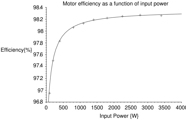
The Biel solar motor user manual (Vezzini & Jeanneret, 2005) provides some measurement data about the efficiency of the motor as a function of input power. This data is shown in fig. 2.6. A simple numerical approximation has been made and given in eq. 2.21.

ηm=

196.7

π arctan(0.25(Pin+ 100)) (2.21)

This function is also plotted in fig. 2.6.

Motor efficiency as a function of input power

96.8 97 97.2 97.4 97.6 97.8 98 98.2 98.4

Efficiency{%}

0 500 1000 1500 2000 2500 3000 3500 4000

Input Power {W}

Figure 2.6: Approximation of the efficiency of the Biel Solar Motor 2005 (BM-5) as a function of input power according to expectations

Although the motor efficiency varies with the motor input power, it is fairly constant (ηmotor = 98.2%) for values of>1000W.

2.3

Insolation

In this section, the input power implementation is treated. Input power is the amount of power collected by the solar panels. This quantity depends on the efficiency of the solar cells (ηp), the efficiency of the

Maximum Powerpoint Trackers1_η

mppt, the effective panel surface (A), the maximum insolation (Isol)

and the angle of the sun above the horizon (γ).

This section starts with explaining the general input power (insolation) equation, which is imple-mented in the ’Insolation equations’ submodel in Fig. 2.2. Subsequently, it treats the calculation of the maximum insolationIsoland the angle γ, which is basically the implementation of the Sun submodel

in Fig. 2.1. After this, the MPPT’s are briefly explained. This section finishes with a test run of the calculation of the insolation for each moment in time during 1 day.

1

INSOLATION 15

2.3.1 General Insolation

Insolation consists of 3 types of insolation of which ’Direct Beam’ and ’Diffuse’ insolation are the most important.

Direct Beam Direct Beam Insolation is sunlight that arrives at the solar panels in a straight line from

the sun.

Diffuse Diffuse Insolation is indirect insolation due to the scattering of sunlight caused by dust, clouds,

haze, fog etc. Diffuse sunlight is unfocused light, which comes from everywhere.

Reflections Sunlight reflected by earth and surroundings (buildings etc.). As this type of insolation

is unlikely to be very large compared to Direct Beam and Diffuse Insolation (the solar array is directed to the sky, so surrounding reflections are unlikely to reach the array), it will be neglected.

The input power equation is (Trottemant, 2004):

Pin=ηp·ηmppt·A·(IDirect+IDif f) (2.22)

Although direct beam insolation is relatively easy to calculate, diffuse light insolation is not. The following approximation forPinis used by (Trottemant, 2004) (eq. 2.23):

Pin=ηp·ηmppt·A·

SC_·sin(γ) + (1₋SC)_·CB_·Isol(γ) (2.23)

In whichSCis the ’Sun Coverage’ percentage, which is the amount of irradiance that is not blocked by clouds etc. CB is the ’Cloud Brightness’ percentage, which represents the ’haziness’ and the level of cloud refraction. γ is the angle of the sun above the horizon, whileIsol(γ) is the maximum insolation

due to atmospheric scattering and absorption, which depends on the observer’s position, the time of the day and the time of the year.

The sun coverage and cloud brightness parameters will have to be predicted before optimization. They can be measured for analysis afterward.

2.3.2 Maximum Insolation (Sun submodel)

The maximum InsolationIsol(γ)depends on the angle of the sun above the horizon (altitude angleγ). If

γis small, solar rays will have to travel a larger distance through the earth’s atmosphere, while attenuated by scattering and absorption.

The effect of atmospheric attenuation can be calculated using the definition of ’Air Mass Index’, which is a measure of the amount of air the sun rays have to travel through ((Liu, 2001)). The maximum insolation is approximated by (Liu, 2001 (Liu, 2001)):

Isol(m) = 1353·0.687m

0.678

{W/m2_} (2.24)

in which

m= 1

sin(γ) (2.25)

The altitude angleγdepends on location (longitude & latitude), the earth’s declination, the time of year etc. In the same paper, a calculation of the angleγ is provided:

16 2. SOLAR CAR MODEL

Solar Irradiance

0 5 10 15 20

time {hr} 0

200 400 600 800

1000 Solar_Power {W/m2}

Summer

25 Sept.

Winter

Figure 2.7: Solar Irradiance (Isol(γ)·sin(γ)) at mid-summer (December 21), mid-winter (July 21) and

at the 25th of September (start of the race)

withHthe hour angle,latthe latitude anddeclthe declination of the earth.

H = 360

24 [N−th−h0] {deg} (2.27)

N = 12 + EOT

60 +

ψlocal−long

15 {hr} (2.28)

decl = 23.45_·sin

2π284 +d 365

{deg_} (2.29)

with N the local noon time, EOT an ’Equation of Time’2 , long the longitude, ψlocal the local

meridian,th−h0the time difference from solar noon time and, finally,dthe day of the year (32 = 1st of

February).

The result (Isol(γ) sin(γ)) as a function of time is shown in fig. 2.7. Insolation is plotted for three

different days of year (at Alice Springs, AUS, app.130◦_long.,

−20◦_{lat.). The difference between winter}

time and summer time is distinct.

2.3.3 MPPT’s

The Solar car is equipped with New Generation maximum powerpoint trackers (MPPT’s). These devices track the so-called maximum power point, which is the point at which the power transferred to the load (fig. 2.8(b)) is maximum. The MPPT device changes the input/output current ratio by varying the output voltage until the maximum power point_{Vmpp, Impp}has been found (fig. 2.8(a)).

The MPPT that is used by the solar team is the MPPT New Generation of the University of Applied Sciences of the Biel School of Engineering (Biel School, 2003), which is a 200/800W DC/DC Maximum Power Point Tracker with boost converter meaning that the output voltage is always higher then the input voltage. 5 MPPT’s are used simultaneously in the solar car.

The MPPT functions optimally with an input power of between 200 and 800W at temperatures be-tween 0 and 70 degrees Celsius. The optimal efficiency of the MPPT is 98.8% at an output voltage of

2

An approximation of theEOTis:EOT = 10.2 sin(4πd−80

373 )−7.74 sin(2π

d−8

355) ∼

= 0.34(d−268)+8.2 d∈[268,277]

INSOLATION 17

I

V

(a) Photo-voltaic cell characteristic

SolarCell Load

(b) Single Solar cell with load

Figure 2.8: Single solar cell curve and connection circuit

130 V, an input voltage of 110 V and an input power of 300 W. The MPPT efficiency for a single MPPT as a function input power is shown in fig. 2.9.

MPPT

0 100 200 300 400 500 600 700 800

MPPT Input Power 0 10 20 30 40 50 60 70 80 90 100 0 10 20 30 40 50 60 70 80 90 100 -4 -2 0 2 4 6 8 10 12 14 16 approximation (%) MPPT eff. (%) error (%)

Figure 2.9: MPPT efficiency as a function of input power and the approximation

The MPPT efficiency curve can be approximated by:

ηmppt= 100 arctan(0.225Pin)−0.003Pin+ 0.8

However, the MPPT efficiency can be considered constant over a wide range (input>100 W). It is only when input becomes lower then 100 W, that MPPT efficiency significantly decreases.

2.3.4 Input power testing

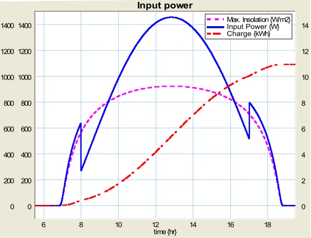
Fig. 2.10 shows the results of the implementation of eq. 2.23. The input power is calculated for the 25th of September at the location of Darwin, NT, with a Sun CoverageSCof 100%, a panel efficiencyηp of

23%, an MPPT efficiencyηmpptof 98% and a solar array areaAof 7 m2(values provided by Electrical

18 2. SOLAR CAR MODEL

Input power

6 8 10 12 14 16 18

time {hr} 0

200 400 600 800 1000 1200 1400

0 200 400 600 800 1000 1200 1400

0 2 4 6 8 10 12 14 Max. Insolation {W/m2} Input Power {W} Charge {kWh}

Figure 2.10: Input power simulation. This figure shows the Maximum InsolationIsol(t), the resulting

input powerPin(t)and the total collected energy during one day of charging. The location is Darwin,

NT, and the Sun CoverageSCis 100%.

The figure shows that a maximum input power of slightly more than 1400 W and a total amount of collected energy of ca. 11 kWh can be achieved on a cloudless day. The figure also shows discontinuities at 8 a.m. and 5 p.m. These result from the regulation that cars are only allowed to drive between these moments. Before 8 a.m. and after 5 p.m., the team is allowed to point the solar array directly at the sun ( orsinγ = 1).

However, clouds at the horizon, imperfect aiming of the array at the sun and decreasing MPPT efficiency may cause lower input power. So the input power calculation is multiplied with parameterηec

which models the effectiveness of these charging sessions before and after racing time.

2.4

Batteries

The solar car model is built up of a simple battery, which stores the energy surplus, or makes up for an energy deficit.Pinis the power gained from the solar panels, which is already already defined in eq. 2.23.

Poutis the power used for driving the car, which is the sum of all power lost to friction, resistors (e.g.

motor efficiency) and other power consumers (P0), like the radio and the sensors.

Q(t) =Q(t0) +

Z t

t0

(Pin−Pout)dt (2.30)

BATTERIES 19

2.4.1 Worley’s lithium polymer cells

The solar car batteries are Worley Lithium Polymer cells, produced by KOKAM. These batteries have a very high energy density (0.180kW h_{/kgwhich makes them very attractive for usage in solar cars, where}

mass is considered to be a critical parameter.

The Worley battery is a 3350 mAh battery cell. The battery pack of the solar car consists of enough cells to hold at least 5 kWh of energy, with a maximum weight of 30 kg. in accordance with the regula-tions.

Also, the efficiency of this type of battery contributes to the attractiveness of lithium polymer batter-ies. When used properly, 99% of the energy stored in the battery can be recovered.

2.4.2 Battery SOC measurement

One of the hardest quantities to measure of the solar car is the battery State-of-Charge, which will have to be measured indirectly, by keeping track of the battery current. The battery state-of-charge is the time-integral of the battery current.

Using a current measurement to keep track of the battery SOC, however, will be inaccurate as each offset on the current measurement is accumulated, causing drift in the SOC measurement.

The output voltage of the battery is not a good measurement of the battery SOC either, as is shown by the discharge current curves of the Worley lithium polymer cell (Worley, 2004) in fig. 2.11. This figure shows the battery output voltage at various constant discharge current rates. As the solar car typically does not use constant battery currents, these output voltage curves cannot be used for battery SOC measurements.

20 2. SOLAR CAR MODEL

A solution to this problem is to use a highly accurate current sensor for battery current measurements in combination with a periodic calibration of the battery SOC measurement. The measurement can be calibrated by using an ’equilibrium curve’.

Battery states

According to (Valer Pop, 2005) a battery or accu can be in one of the next 4 states:

Charge Battery SOC increases, caused by an input current;

Discharge Battery SOC decreases, caused by an output current;

Transit Battery current has decreased below 0.05 CmA, either charging or discharging;

Equilibrium The battery enters equilibrium state after being in Transit state for at least 2 hours,

de-pending on the type of battery.

When in equilibrium state, the battery SOC can be estimated with fair accuracy by measuring the output voltage and correcting for battery temperature (the accu pack used in Australia contains tempera-ture sensors). In that case, the plot of fig. 2.11 is again used, with the discharge current curve of<0.05 CmA, which can be gained by extrapolating or, better, measurement. In that case, a discharge curve of at most 0.05 CmA should be used (taking 20 hours to fully discharge).

Example

Suppose a electric device that requires a constant supply current of, conveniently, 0.5 CmA. The battery output voltage will behave like the 0.5 CmA curve in fig. 2.11. After 4 hours of continuous discharge (2000 mAh), the battery output voltage will be approximately 3.63 V.

If the device is shut down, the battery will enter transit state. if the device is not powered up in the next 2 or 3 hours, the battery will slowly enter equilibrium state: the battery output voltage will rise slowly until the equilibrium curve is reached, where it will settle.

Extrapolating from the curves, that have already been measured, the equilibrium curve will be ap-proximately 3.9 V.

Australia

When using these batteries during the solar challenge race, the battery SOC are estimated by using voltage and current measurements. Calibrating the SOC measurement can be done each day after having had a whole night to enter the equilibrium state and before the racing starts at 8 ’o clock in the morning. When calibrated, the initial battery State-of-Charge is known and a new strategy can be developed. However, temperature does have its effect on the equilibrium curve, so the initial state-of-charge mea-sured may not be very accurate ((Worley, 2004), sheet 9).

2.4.3 The SolUTra battery

Measurement

TESTING THE SOLAR CAR MODEL 21

75 80 85 90 95 100 105

0 1 2 3 4 5 6

Battery charge (kWh)

B

a

tt

e

ry

o

u

tp

u

t

v

o

lt

a

g

e

(

V

)

Equilibrium Curve (3A Charge) Extrapolation of linear area

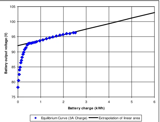
Figure 2.12: Equilibrium curve of the SolUTra racing battery pack, using a charge current of 3 A∼=0.04 CmA. Only half of the measurements were performed. The extrapolation is also shown.

Worley lithium-polymer battery cells in parallel. In the days before the 25th of september 2005, the battery cells were properly balanced and the battery equilibrium curve was measured, using a charge current of exactly 3A, which is slightly less than 0.05 CmA. Due to circumstances, the charging time was limited to approximately 10 hours, so only half of the equilibrium curve was measured (Fig. 2.12).

When leaving Darwin during the World Solar Challenge, the battery was fully charged to 6.2 kWh.

Extrapolation

Extrapolating the equilibrium curve for>2.5 kWh is prone to inaccuracy, as the sensitivity kW h_/Vis

large, due to the fact that the equilibrium curve for>0.5 kWh is relatively flat. In absence of a reliable equilibrium curve for SOC>2.5 kWh, the extrapolation of fig. 2.12 is used.

2.5

Testing the Solar Car Model

2.5.1 Model

Summarizing, the solar car model equations are

Q(t) = Q0+

Z t

t0

(Pin−Pout)dt

x(t) = x0+

Z t

t0

vcar(t)dt

22 2. SOLAR CAR MODEL

Quantity abbr. value unit source Car parameters.

Aerodynamic profile (est.) CW(δ) 0.08 - Estim. by Aero. div.

Vel.-indep. roll fric. coef. cr1 0.0023 - (Tamai, 1999)

Vel.-dep. roll fric. coef. cr2 4.1·10−5 (m/s)−1 (Tamai, 1999)

Car mass mc 280 kg Estim. by Mech. div.

Solar Panel eff. ηp 23 % Estim. by Elect. div.

MPPT eff. ηmppt 98 % section 2.3.3

Solar Panel Surface A 7.092 m2 _{Estim. by Elect. div.}

Default Motor eff. ηm 98 % section 2.2.4

Other parameters.

Regen. brake eff. ηrb 60 % Estim. by Elect. div.

Charge effectiveness ηec 70 % section 2.3.4

Default Air density ρ 1.17 kg_/m3 _{section 2.2.1}

Number of wheels n 3 - Observation

Const. Power factor P0 ∼23 W Estim. by Elect. div.

Local meridian ψlocal 127.5 ° +9.5 Time zone

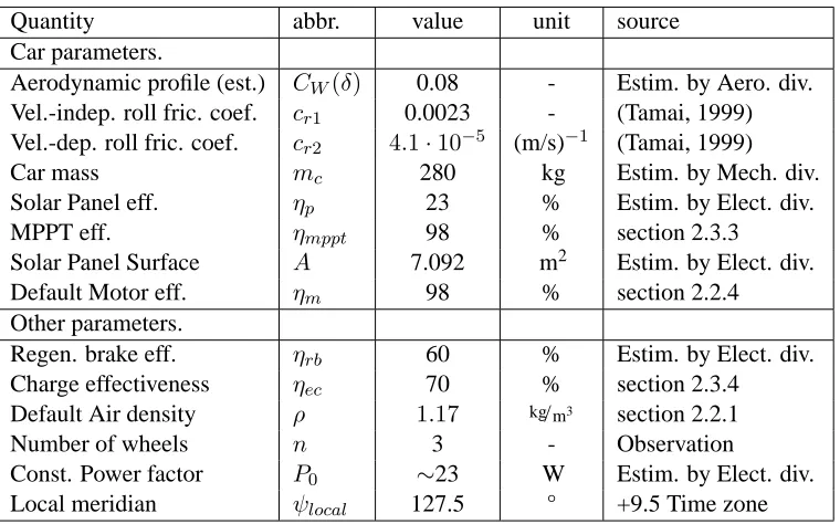
Table 2.1: (constant) Car parameters (of which some are estimations by various divisions of the Solar Team). The primary car parameters are the most important characteristics of SolUTra.

The equations for input and output power are

Pin = ηp·ηmppt·A·

SC_·sin(γ) + (1₋SC)_·CB_·Isol(γ)

Pout = P0+

1

ηm

1

2ρCW(δ)·v

2

ef f +mcg·(sin(α) +n·cr2)·vcar+mcg·cr1

·vcar

In this case, the motor efficiency is assumed to be constant. However, the motor efficiency varies with the motor speed and torque.

2.5.2 Parameters & Characteristics

The car parameters are summarized and quantified in table 2.1.Some of the parameter values in this table have been obtained from contact with team members of the Solar Team University of Twente and are therefore indications of the real parameter values.

With these values the following output power characteristic can be derived (fig. 2.13).

From this figure, it can be derived that with this parameters, the roll friction exceeds air friction when the car speed is lower than 50 km/h. Above 50 km/h, air friction is the dominant friction factor. A characteristical value is the output power at 100km_{/h, which is ≃ 1500 W for the SolUTra in this}

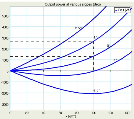
configuration. This is a relatively low value, when compared to the 1650 W of the NUNA III, this year’s champion (van Velzen, 2005), so the car is either very good, or the car parameters may be very optimistic. The output power is plotted in fig. 2.14 for various slopes. It can be seen that output power doubles between 80 and 100km_/hin case of a 1° slope, suggesting the importance of measuring the slope of the

TESTING THE SOLAR CAR MODEL 23

Output Power

0 20 40 60 80 100 120

Car Speed {km/h} 0

500 1000 1500 2000 2500

Pout {W} Pdrag {W} Proll {W}

Figure 2.13: Output power and components as a function of car speed on a flat road with no wind

Output power at various slopes (deg)

0 20 40 60 80 100 120 140

x {km/h} -3000

-2000 -1000 0 1000 2000 3000 4000 5000

Pout {W}

2.5°

1°

0°

-1°

-2.5°

Figure 2.14: The total output power (including drag and roll friction) at various slopes. Between 80 and 100km_{/h, a slope of1}◦

Chapter 3

Strategy Optimization

A man who does not plan long ahead will find trouble right at his door. – Confucius

3.1

Introduction & Optimization Problem

In this chapter, the optimization problem (OP) and the ways to solve this problem are treated. The chapter starts with a description of the optimization goals. These goals are translated into a Cost Criterion function. Then, some methods for optimization are treated. In the last section, a possible implementation of optimization in PALLAS is suggested.

The emphasis of developing a strategy is on finding an optimal solution to the OP in a fast and reliable way.

For simplicity, car speed is now represented byv(t)instead ofvcar(t).

3.1.1 Optimization goals

Speed

The OP that is to be solved by the SDP is basically a time-optimal control problem and a minimization (eq. 3.1) of the timeteneeded to travel a certain distancextotal, which is the total distance from start to

finish.

minJ =

Z te

0

dt=te (3.1)

The solution to this OP is the highest average car speed achievable. During the race, input and output power are to be carefully balanced, as the only power available for driving is gained from the solar panels and no other power source may be used.

Efficiency

The car’s efficiency is measured by the energy used to move the car over a fixed distantxtotalin a fixed

amount of time te. This can be translated to displacing the car with a limited amount of energy in a

certain amount of time. Maximizing efficient use of available energy means therefore minimizing eq. 3.2.

minJ =

Z te

0 −

26 3. STRATEGY OPTIMIZATION

Solution to the Optimization problem

The Solar Car model, which is designed in chapter 2, is used for calculating the results of various strate-gies. The input of this model is SolUTra’s car speedv(t). The eventual solution to the OP will therefore be an optimal car speed functionv∗_(t).

3.1.2 Criterion & optimization constraints

The criterion is to be designed while keeping a close eye on the requirements of the method that is used to optimize the racing strategy.

Constraints

The solar car has a strict constraint on battery usage: the battery SOC is not allowed to be less then 0 kWh, nor is it allowed to exceed the maximum charge of approximately 6.2 kWh (section 2.4.3). It is recommended to stay away from these limitations, as empty batteries result in the unfavorable situation that the driver is restricted to a low maximum car speed (depending directly on input power) and fully charged batteries result in a situation in which the energy surplus cannot be stored.

Uncertainty in weather expectations, road measurements, or parameter estimations may cause situa-tions as described above. These situasitua-tions can be avoided by using ’safety regions’: the normal ’opera-tional range’ of the battery is set to be between ca. 10% and ca. 90% of full battery charge. In the event of getting more or less solar energy then expected, these safety zones guard the occurrence of unfavorable situations. Using the safety zones should be punished when calculating an optimal racing strategy

These safety zones do not apply in the vicinity of either start and finish. At the starting line, the batteries are allowed to be completely charged. At the finish line, however, efficient use of energy demands the batteries to be almost exhausted, as energy left-overs could have been used for more speed. Apart from battery SOC constraints, there are some other aspects that may constrain optimization:

Speed limits Speed limits apply to parts of the road between Darwin and Adelaide. These speed limits

vary from 50, 60 or 80km_{/hin towns and cities, while a maximum speed of 110}km_{/happlies to the}

whole of the state of Southern Australia. Serious cases of speeding may lead to disqualification;

Battery discharge current The battery SOC depends on the discharge current: larger discharge currents

wear the battery. So, large discharge currents should be avoided;

Motor efficiency Each motor has a region in which efficiency is optimal. Using that region as much as

possible is an energy efficient way of driving. Especially when using a direct-drive motor, as no transmission is used to keep the motor functioning optimally efficient;

Choosing camping sites Choosing a camping site at which the car can still collect solar energy at the

end of the day will result in better initial conditions for the day after. This may be implemented by imposing penalties on certain values ofx(te), but this will also generate local minima,

complicat-ing global optimization.

Optimization Parameters: Stages & time steps

As already stated, the result of the optimization should be an optimal car speed functionv∗_{(x, t)}

. To calculatev∗

INTRODUCTION & OPTIMIZATION PROBLEM 27

is complex, and cannot be solved by symbolical computer programs like MAPLE (Schutyser, 2005). Instead, Schutyser (Schutyser, 2005) suggests solving the OP numerically. Pudney (Pudney, 2000), however, has solved the OP analytically (which is briefly explained in appendix C), but he had to rely on shot methods to find the optimal starting conditions and concluded that his analytical solution to the OP was an improvement of mere minutes of the strategy of maintaining a constant speed for the complete distance of the race.

Trottemant (Trottemant, 2004) suggests the use of stages for numerical optimization: the complete distance is divided in a certain number of stages. For each stage, a constant optimal average speed

v∗_{(x)is calculated. In this way, a set of optimization parameters is created, which consists of as many}

parameters as there are stages. The benefits of using stages are:

• Improved calculation speed:

– v(x, t)is simplified to a vector of constants (~v).

– Optimization over a smaller distance or time interval takes less time, as the set of optimization

parameters is smaller.

• The number of stages, and the distribution of stages over the racing track may be changed accord-ing to the most recent situation (changaccord-ing weather etc.);

• Whenx(te)is fixed (end value problem), the number of optimization parameters is constant, thus

avoiding situations in which parameter values do not have effect on the cost criterion at all, result-ing in an infinite set of local minima.

Schutyser (Schutyser, 2005) suggests the use of time steps: vcar(t) is discretized to v(k) with a

certain time steptk. For each time step, an optimal value ofv(k)is calculated. The set of optimization

parameters consists of as many elements as there are time steps. The benefits of using time steps are:

• The size of the time steps can be chosen beforehand. The size can even be variable during the race (like variable sized stages);

• Using time steps resembles discretization of a continuous input signal, rather then using stages;

• Whente is fixed, the number of optimization parameters is constant, thus avoiding situations in

which parameter values do not have effect on the cost criterion at all, resulting in an infinite set of local minima.

However, media-stops (30-minute stops at certain locations) during the trip may complicate the use of time steps as optimization parameters.

Time and distance are related viax(t) =R

v(t)dt. However, when speed is considered to be constant during one stage or time-step, the interdependence can be simplified to:

xk =vktk (3.3)

in whichvk designates thek-th car speed element in the optimization parameter set and tk is thek-th

time step.xkis the distance traveled during thek-th time step or stage.

When considering time steps and stages, stages are fitted for use when optimizing car speed for a fixed distance (being as fast as possible), while time steps can be used when car speed is to be optimized over limited timete (being as fast as possible, as well as being as efficient as possible). After all, an

28 3. STRATEGY OPTIMIZATION

a certain optimization parametervi(the ith timestep) does not influence the cost criterion, or (withV the

set of feasible car velocities).

dJ

dv(i) = 0∀vi ∈ V

This is the case, when the ith timestep starts aftert=te.

Optimization Criterion

The cost criterion is the function that is evaluated by the optimization method to decide which set of optimization parameters is optimal. The optimization method may require the evaluation function to meet certain specifications. Most gradient methods (see B.2.2) require the evaluation function to be twice differentiable.

The fundamental optimization criteria have already been given in equations 3.1 and 3.2. These crite-ria are extended with a functiong(Q(t)), which represents the battery safety limits, which are described in section 3.1.2.

Also a factor w4(Q(te)−Q2_des is included in the criteria. This factor can be used when a certain

battery SOC end value is desired for setting intermediate goals. e.g. In case of optimizing for one day only. It may be desired to have, for example, the batteries charged for 60% at the end of the day.

Using stages, the goal is basically to travel a certain distance in as little time as possible. So,x(te)is

fixed andteis minimized. The optimization criterion is then (using vector of weightsw~):

J(vcar) =w4(Q(te)−Qdes(te)2) +

Z te

0

(w1+w3·g(Q(t)))dt (3.4)

If a fixedteis considered,x(te)is to be optimized, soJ2 includes an integral of the car speedv.

J(v) =w4(Q(te)−Qdes(te)2) +

Z te

0

(₋w2·v+w3·g(Q(t)))dt (3.5)

In both equations,g(Q(t))is defined as:

g(Q(t)) =







(Q(t)₋Q−₎2 _{Q(t)< Q}−

(Q(t)₋Q+

)2

Q(t)> Q+

0 otherwise

(3.6)

whereQ−

andQ+

represent the lower resp. upper battery safety limits. The function penalizes exceeding the battery safety limit quadratically, because this function is twice differentiable. This function is illus-trated in fig. 3.1 and explained in appendix B.2.4. Using eq. 3.6, constraints (such as0_≤x(t) _≤x(te)

andvi>0) can be changed into penalty functions as well.

3.2

Optimization methods

3.2.1 Cost Criterion: Example

OPTIMIZATION METHODS 29

0 1 2 3 4 5

0 1 2 3 4 5 6 7 8 9 10 SOC {kWh} g(Q)

Figure 3.1: The safety regions of the battery. Including this function will prevent using those regions.







J =w1Pn_i=1x_vi

i +w2·

Pn

i=1

xi

vi[Pin(xi, t)−Pout(xi, vi)]−Qdes

2

Pin≥0;Pout >0;xi, vi >0;Pni=1xi =C

(3.7)

in which cost criterionJ1 depends solely on the end values of the car states (battery safety region is

not included).

A graphical representation of the cost criterion may be produced by setting up an experiment, consist-ing of a 100 km race. Durconsist-ing this race, the input power is assumed to be constant, as well as disturbances, like wind, which is assumed to be constant during a single stage.

The race consists of 2 stages of 50 km. each. A constant car speed is chosen for each stage. In fig. 3.2(a) the cost criterion for10< v1, v2 <100m/s is plotted, showing a single minimum. Obviously, the

cost criterion is not defined forv1 ≤0Wv2 ≤0, as these cases prevent the car from reaching the finish

line. Optimization Criterion 0 50 100 150 200 250 20 40 60 80 100 v2 20 40 60 80 100 v1

(a) Cost Criterion

2nd order Derivative test

–0.02 –0.01 0 0.01 0.02 20 40 60 80 100 v2 20 40 60 80 100 v1

(b) 2nd Derivative test

Figure 3.2: The end values of cost criterionJfor 2 stages resp. 2 timesteps optimization with MAPLE.

However, the plot also shows that near the axes (v1,2 → 0), the plot tends to decrease. This effect

30 3. STRATEGY OPTIMIZATION

derivative test’ (Weisstein, 1999b).

D=

∂2_J

∂v2 1

∂2_J

∂v1∂v2

∂2_J

∂v2∂v1

∂2_J

∂v2 2 (3.8)

This test shows the region in which gradient-based optimization methods will converge (D >0), and in which they will diverge (D <0). TheD = 0curve is also plotted in fig. 3.2(b). This curve moves and scales with variations in racing conditions (slopes, wind etc).

When optimizing, especially when using a gradient optimization method, regions in whichD < 0

must be avoided, as gradient methods will diverge from the optimal solution in these regions.

To avoid diverging gradient methods, the battery safety region of eq. 3.6 is used to keep the battery state of charge within acceptable and safe limits like a penalty function. This function is continuous and twice differentiable, which is required in order to calculate the Hessian.

Including the battery safety regions generates the cost criterion surface plane of fig. 3.3(a). In this figure,J1 (eq. 3.4) is plotted for the same racing experiment of fig. 3.2(a). Even exceeding the battery

10 15 20 25 30 35 40

10 15 20 25 30 35 40 v1 (m/s) v2 (m/s) 0 10 20 30 40 50 60 70 80 90 (a) Stages

10 15 20 25 30 35 40

10 15 20 25 30 35 40 v1 (m/s) v2 (m/s) 0 10 20 30 40 50 60 70 80 90

(b) Time steps

Figure 3.3: 2 stages optimization with MATLAB, including battery safety regions.

safety limits for just a little time causes the cost criterion to skyrocket. The area in which the optimal parameter values are located is clearly visible as a long narrow tinted area. While the derivative of the function large outside of this area, it tends to decrease fast when approaching the optimal solution.

Although all circumstances are equal during both stages, the MATLAB results show that the ’optimal area’ around the optimal solution is not symmetric: J(v1, v2) =6 J(v2, v1). This is caused by the fact

that the input power is not zero, which causes battery overflow in case of driving too slow. Therefore, it does matter whether one drives slow at first or at last.

Also shown is a plot ofJ2(eq. 3.5) in whichte= 2 h. This two-hour race is divided in two (n= 2)

OPTIMIZATION IN PALLAS 31

3.2.2 Optimization

Schutyser (Schutyser, 2005) has treated a similar problem which consisted of a great number of opti-mization variables and a non-linear cost function. Schutyser (Schutyser, 2005) distinguishes 4 types of optimization problems:

Linear programming problem The cost criterion is linear (or affine);

Quadratic programming problem The cost criterion is quadratic and the constraints are linear or affine;

Non-linear optimization problem The cost criterion is non-linear, non-convex;

Convex optimization problem The cost criterion is a convex function (see section B.1 for the concept

of Convexity).

The cost criteria (both eq. 3.4 and 3.5) are non-linear and convexity cannot easily be proved for a large or infinite number of optimization parameters (Convexity for n _{→ ∞}). Therefore, the OP is considered to be non-linear non-convex and the calculational advantages of the other types cannot be used in this case.

To find the optimum of the OP in fig.3.2.1, a numerical optimization method is needed, that is able to cope with a non linear model and a cost function that is not convex, and which cannot be guaranteed to have only one minimum.

3.2.3 Global Optimization

Some methods for global optimization are given in sectionB.3.

Figures 3.3(a) and 3.3(b) show that, for 2 optimization parameters, the cost criteria (J1andJ2) each

have only one minimum. In that case, the local minimum that is found is also the global minimum. However, for more then 2 optimization parameters, global optimality cannot be guaranteed.

Thus, global optimization should be given special attention. As one of the design goals is calculation speed, methods such as genetic algorithms are generally ruled out. Promising methods are:

Multiple start Optimizing multiple times with varying initial parameter values;

Parameter sweep Evaluate various initial positions and use the best one for optimization (scatter shot).

Both methods benefit from using less function evaluations. Both methods, however, merely increase the chances of finding the global optimum; they cannot guarantee global optimality.

3.3

Optimization in PALLAS

When designing an optimization algorithm for PALLAS, the design specifications of section 1.2 must be observed: optimization should be fast and reliable and flexible.

3.3.1 Design choice: Splitting strategies

32 3. STRATEGY OPTIMIZATION

To increase the strategy development speed, 3 different strategies are used. Developing a strategy for the total remaining distance to Adelaide generally takes a lot of time, compared to developing a strategy that lasts to the end of the day. Primary and secondary goals can be set, the primary being the total race time from Darwin to Adelaide and the latter being at a certain location at the end of the day.

To put it simply: instead of continuously optimizing for the total distance of the race, a strategy is developed for only a part of the race.

Start to Finish: Fixed distance (Long Term Strategy)

Considering the complete distance from start to finish, this distance has to be covered as soon as possible. The total racing timetehas to be minimized, while the battery SOC (Q(t)) is constrained (Battery SOC

may not exceed battery limits and should have a certain value att=te).

For Start-to-Finish optimization, Q(te) should be