Volume 2010, Article ID 969751,12pages doi:10.1155/2010/969751
Research Article
CFAR Detection from Noncoherent Radar Echoes Using
Bayesian Theory
Hiroyuki Yamaguchi and Wataru Suganuma
Air Systems Research Center, Technical R & D Institute, Ministry of Defense, 1-2-10 Sakae, Tachikawa, Tokyo 190-8533, Japan
Correspondence should be addressed to Hiroyuki Yamaguchi,[email protected]
Received 1 July 2009; Revised 12 December 2009; Accepted 11 February 2010
Academic Editor: Martin Ulmke
Copyright © 2010 H. Yamaguchi and W. Suganuma. This is an open access article distributed under the Creative Commons Attribution License, which permits unrestricted use, distribution, and reproduction in any medium, provided the original work is properly cited.
We propose a new constant false alarm rate (CFAR) detection method from noncoherent radar echoes, considering heterogeneous sea clutter. It applies the Bayesian theory for adaptive estimation of the local clutter statistical distribution in the cell under test. The detection technique can be readily implemented in existing noncoherent marine radar systems, which makes it particularly attractive for economical CFAR detection systems. Monte Carlo simulations were used to investigate the detection performance and demonstrated that the proposed technique provides a higher probability of detection than conventional techniques, such as cell averaging CFAR (CA-CFAR), especially with a small number of reference cells.
1. Introduction
Noncoherent radar systems are widely used in applications such as ship navigation, and radar signal detection from sea clutter has been the subject of intense research for a number of years. Considerable experimental and theoretical investigations have studied the feasibility of detection with a constant false alarm rate (CFAR). In CFAR detection, the local sea clutter power in a range cell under test (CUT) is adaptively estimated from samples adjacent to the CUT, which are referred to as reference cells. The estimation method is very important for detection probability enhance-ment, and many studies have been reported.
For example, if the radar illuminates a large sea area, then the probability distribution of the envelope of sea clutter is approximated by a Rayleigh distribution [1]. Thus, the sea clutter in a noncoherent radar system with a square law detector is exponentially distributed. In this sea clutter, the local mean clutter power is spatially a constant (i.e., homogeneous clutter). The local clutter power can then be estimated by the maximum likelihood (ML) method. CFAR implemented using ML is known as cell averaging CFAR (CA-CFAR) [2,3]. If the clutter power varies spatially (i.e., heterogeneous clutter), however, a K distribution provides a good phenomenological expression of the sea clutter,
especially for high-resolution radar at low-grazing angle [4–
9]. Using CFAR detection againstKdistributed clutter, the maximum a posterior (MAP) or the minimum mean square error (MMSE), that is, Bayes risk minimization method, can be applied for the clutter power estimation [10, 11]. By implementing these estimation methods, the spatial correlation of the clutter power is regarded as strong. Thus, the assumption can be made that the local clutter power in the CUT equals that in the reference cells.
example, identify closely separated ships or a ship near land, compared with conventional CFAR using a large number of cells [13].
In this study, a CFAR detection technique is introduced for heterogeneous sea clutter with a noncoherent radar system, where the local clutter power in the CUT is estimated by the Bayesian theory. Typically, this requires sufficient prior information about the sea clutter to be incorporated in the estimation, or the estimation accuracy might be degraded, as with ML and MAP. In the proposed technique, however, CFAR detection is achieved without this prior information. A Bayesian optimum radar detector (BORD) has been reported [14] as one application of CFAR to Bayesian theory. However, the BORD is a coherent radar system and is difficult to implement with a noncoherent system, since complex data, such as the Doppler frequency, is not available. To investigate the detection probability of the proposed technique, Monte Carlo simulations are performed under various sea clutter conditions, including consideration of the spatial correlation of the clutter power. The results are also compared with conventional CFAR techniques, such as CA-CFAR, and show the usefulness of the proposed technique, especially for a small number of reference cells. In the proposed technique, data from the square law detector is processed, allowing easy implementation in existing noncoherent radar systems, such as marine radar, making it particularly attractive for an economical CFAR detection system. In addition, the proposed technique can be applied to high resolution radar, with a range resolution of 4 m [5,8], since heterogeneous clutter is supposed.
In the next section, the clutter and the target signal model are described and then the proposed detection technique. In
Section 3, the detection performance with various clutters is investigated. Finally,Section 4concludes this study.
2. Detection Technique
The detection problem of interest here is that if we suppose a noncoherent radar to transmit a pulse and receive the radar echo. The echo is then detected via a square law detector and sampled by an A/D converter. Here, the sampled echo in the CUT and the echoes fromMreference cells are denoted as XandD= {X1,. . .,XM}, respectively, as shown inFigure 1.
Note that cell size adaptation with respect to the target size is outside the scope of this study. When the target signal is absent from the CUT, it is assumed thatXconsists of only the clutter; when the signal is present, it is assumed that X consists of the sum of the clutter and the target signal and is statistically independent of the clutter. Additionally, the system noise is sufficiently small compared with the clutter and is neglected. Note that information about the sea clutter is not available, since the sea clutter’s statistical characteristics might change frequently with factors such as the wave structure.
2.1. Sea Clutter and the Target Signal Model. Assume that the sea clutter is heterogeneous and modeled as the compound Gaussian, as described in [6,7,10,15]. From these references,
the clutter C can be represented by the product of two independent random variables
C=τx, (1)
wherexandτ are named speckle and texture, respectively. The variable x is given by a noncorrelated exponential random variable. The variableτ represents the local clutter power, that is, the mean of the underlying conditional exponential distribution.
In general, local clutter power fluctuations are induced by spatial and temporal variations in the clutter. Their correlation lengths are a few tens of meters and the order of seconds, respectively [9,16]. Because its long temporal correlation time, local clutter power is regarded as a constant during CFAR processing intervals. Thus, modeling the spatial power distribution is important in CFAR detection. In [7], for example, the distribution function of the power is given by a Gamma distribution, that is, the distribution function of the clutter is the K distribution, which is a function of the scale and shape parameters. In this study, the distribution function of the power is given by an inverse Gamma distribution because this is a conjugate prior distribution [17]. By using this prior, a prior and posterior distributions belong to the same class of distributions. Thus, transition from prior to posterior only involves a change in the parameters with no additional calculation, which reduces the computational complexity. We must consider the justification of the inverse Gamma distribution. In the performance analysis in Section 3, the local clutter power of the simulated sea clutter is given as Gamma distributed (not inverse Gamma). To determine the validity of the proposed technique applying the inverse Gamma prior, analysis is performed using simulated sea clutter. The inverse Gamma distribution is also a function of the shape and scale parameters (these parameters differ from those in the Gamma distribution). However, no information about the clutter is available, so the parameters are not known a priori. Generally, atmospheric propagation effects (i.e., clear sky, rain, etc.), target scintillation, and so on, cause the target signal to fluctuate. From a radar specification point of view, the pulse repetition frequency (PRF) is a few kHz, since marine radar is assumed in this study. Thus, target scintillation might be neglected during CFAR processing intervals; the target echo fluctuates slowly relative to the order of magnitude of the PRF. Therefore, the target model is assumed as Swerling I, which has been largely used in radar literature [18]. In this model, signal fluctuation is given by an exponential distribution and the mean of the fluctuation represents the signal power.
2.2. Proposed Technique. Similar to CA-CFAR, the test statisticTin the proposed technique is defined as
T=X
τ, (2)
Antenna
Transmit signal TX
Circulator
Received echo
Square law detector
Range bin Sampled echo
X1 · · ·
Reference cell
Xm · · ·
Guard cell
X
CUT
· · ·
Guard cell
Xm+1· · · XM
D= {X1X2· · ·XM}: Reference cell
Reference cell
Figure1: Data in CUT and reference cell.
comparing T with a threshold level η; if T η (orT < η), the target signal is present (or absent). The threshold is given from the false alarm rate. In addition, the clutter in the CUT and the power are estimated by the Bayesian. With these estimated values, the proposed CFAR detection is formulated. The following explains the estimated values by the Bayesian theory and provides the false alarm rate and the probability of detection.
2.2.1. Local Clutter Power Estimation. Suppose that bothX and D contain no target signal, and that the local clutter power in the CUT is the same as that in the reference cells. Based on Bayesian theory, a posterior distribution of the local clutter power in the CUTτ conditioned onX andD is expressed as
p(τ|X,D)=∞L(τ|X,D)p(τ)
0 L(τ|X,D)p(τ)dτ
, (3)
whereL(τ |X,D) and p(τ) are a likelihood function and a prior distribution of the local clutter powerτ. The likelihood function is given by
L(τ|X,D)=p(X|τ)×
M
m=1
p(Xm|τ), (4)
wherep(X|τ) andp(Xm|τ) are an exponential distribution
conditioned onτ
p(X|τ)=1
τe
−X/τ, p(X m|τ)=
1 τe
−Xm/τ. (5)
The prior distribution, that is, the assumed local clutter power distribution, is the inverse Gamma distribution, as mentioned inSection 2.1. This is denoted byIG(τ;α0,β0),
withα0of the shape parameter andβ0of the scale parameter, that is, hyperparameters. Thus,
p(τ)=IGτ;α0,β0
= β
α0
0
Γ(α0)τ
−α0−1e−β0/τ. (6)
Since the inverse Gamma distribution is the conjugate prior, the posterior distribution p(τ | X,D) in (3) is also the inverse Gamma. Thus, p(τ | X,D) = IG(τ;α1,β1). The hyperparameters are represented by
α1=M+ 1 +α0, (7)
β1=
M
m=1
Xm+X+β0. (8)
Therefore, the distribution of the estimated local clutter powerτbased on the Bayesian theory is given by
p(τ|X,D)=IGτ;α1,β1
. (9)
Next, we have to consider the value of τ to output T in (2). As seen in (9),τis not estimated as the point value but as the distribution. Thus, we propose that the estimated local clutter power is given as a random variable whose distribution is the inverse Gamma, that is,τ ∼IG(τ;α1,β1) (“∼” means “distributed as”). By using a Gaussian random number generator, the estimated local clutter power is given by
τ =
⎛
⎝1
β1
α1
k=1
|nk|2 ⎞ ⎠
−1
, (10)
wherenkis a complex random number, and its statistics are
0 10 20 30 40 50 60 70 80 Threshold levelη
10−8 10−6 10−4 10−2 100
PFA
M=2
M=4
M=8
M=16
M=32
Figure2: Example of threshold level in proposed CFAR.
2.2.2. Hyperparameters. The hyperparameters are not known a priori. Thus, a noninformative prior [17,19,20] that is one of the approaches to obtaining the hyperparameters is considered in this study. By using the noninformative prior, a prior distribution is regarded as uniform. Thus, α0 → 0 andβ0 → ∞should be used. However, the parameters are set toα0 = 1 andβ0 = 0. For the former value, because the estimated local clutter power in the CUT is given by (10) andα1as the summation index, it must be a natural number. From (7),α0 is also a natural number. Therefore, α0 = 1, that is, the smallest natural number, is used. Meanwhile for the latter value β0 = 0 is used (though this should be a large number) because a false alarm rate is to be derived analytically. Ifβ0 is not a zero, the distribution ofβ1is not a Gamma distribution (i.e., the distribution ofY1in (A.5) is not the Chi-square distribution in the appendix). Therefore, it is extremely difficult to derive the false alarm rate. The discussion of detection performance dependence on the parameters is inSection 3.1.
2.2.3. Local Clutter Estimation. In (3),X is assumed as the clutter. However, this assumption cannot be accepted in actual detection scenarios since whetherXincludes the target signal or not is unknown. Therefore, we propose replacing X in (3) with the estimated clutter from the data in the reference cells. The Bayesian theory is also applied for the estimation. The estimated clutter denoted asCis given as the mean of the Bayesian predictive density function (MBPDF). In the MBPDF,Cis represented by
C=
∞
0 CP
∗(C|D)dC, (11)
whereP∗(C | D) is the predictive density [17,19,21,22]. This is defined by
P∗(C|D)=
∞
0 p(C|τ)p(τ|D)dτ, (12)
where p(C | τ) = 1/τe−C/τ and p(τ | D) is the posterior
distribution, that is,p(τ|D)∝L(τ|D)p(τ). The likelihood function is given by
L(τ |D)=
M
m=1
p(Xm|τ). (13)
Since the prior distribution is also supposed as the inverse Gamma distribution with the hyperparameters asa0andb0, that is,p(τ)=IG(τ;a0,b0); the posterior distribution is thus the inverse Gamma distribution,p(τ|D)=IG(τ;a1,b1) with the hyperparameters as
a1=M+a0,
b1=
M
m=1
Xm+b0.
(14)
Substitutep(C|τ) andp(τ|D) into (12), then
P∗(C|D)∝ Γ(a1+ 1) (X+b1)a1+1
, (15)
where “∝” signifies “proportional to.” Therefore,Cis given by
C=A·Γ(a1−1)b−1a1+1, (16) where A is a constant. Since the hyperparameters are not known, the noninformative prior as described in
Section 2.2.2is applied. Thus,a0=0.1 andb0=10 are given. Contrary to hyperparameters α0 and β0 in Section 2.2.2, these values ofa0andb0do not affect a false alarm derivation. With these values, the prior distribution, that is, the inverse Gamma distribution, is approximated as uniform. In the local clutter power estimation inSection 2.2.1, the posterior distribution of the power is then estimated withCinstead of X, that is,Xis replaced withC.
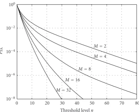
2.2.4. False Alarm Rate and Probability of Detection. The expressions of the false alarm rate PFA and the probability of detectionPD are described in the appendix;PFAandPD are given by (A.11) and (A.13), respectively. Note thatPFA is independent of the statistical parameters of the clutter. Therefore the proposed technique offers CFAR capability with respect to the clutter. Also note thatPFAandPDinclude integration as the confluent hypergeometric function of the second kind [23] and the calculation of the threshold is slightly difficult. InFigure 2, we show examples ofPFAversus ηfor variousM.
Figure 3shows a block diagram of the proposed detection technique. InFigure 3(a), first, the sum ofXmis calculated
from the reference cells, and then the clutter in the CUT is estimated by the MBPDF (the detailed process is shown in
Figure 3(b)). Using the estimated clutter and the sum ofXm,
Received data Square
law detector
X1 · · · Xm X Xm+1· · ·
· · ·
XM
· · ·
Data at CUT,X ΣMm=1Xm
Estimation of clutter at CUT by MBPDF
X
Estimation of local clutter power distribution in CUT by Bayesian theory
α1andβ1 Estimation of local clutter power value
in CUT
τ T
η
Detection
Threshold level
÷
(a) Block diagram.
M m=1Xm
Hyperparameter (a0,b0)
a1=M+a0
b1= M m=1Xm
+b0
MBPDF X∝Γ(a1−1)b1−a1+1
X
(b) Detail flow for the estimation of clutter in CUT by MBPDF.
X
M m=1Xm
Hyperparameter
(α0,β0) α1=M+ 1 +α0
β1= M m=1Xm
+X+β0
nk Gaussian random
value generator
τ
τ=
1
β1 α1 k=1|
nk|2 −1
(c) Detail flow for the estimation of local clutter power in CUT. Figure3: Block diagram of proposed detection technique.
is divided byτ. Finally, the test statisticTis compared with the threshold levelηto determine whether the target signal is present.
3. Performance Analysis
In this section, the detection performance is numerically investigated by Monte Carlo simulations. To determine the validity of the proposed technique when applying the inverse Gamma prior distribution of the local clutter power, the sea clutter in the simulation is given as theK distribution. Thus, the local clutter power is Gamma distributed (not inverse Gamma). The K distribution is a function of the shape parameterνand the scale parameterθ. Generally, the distributions with a small and largeνare far from and close to the exponential distribution, respectively. The mean of the local clutter power is represented by νθ. The local clutter
power is spatially correlated in range and its autocorrelation function is defined as [24]
ACF(i)=E{τmτm+i}
E{τm2} , (17)
where E{·} is an expectation, i is the shift of range cell, andτm is the local clutter power in the range cellm. In this
simulation, the autocorrelation function is given by [25]
ACF(i)=ρi, (18)
whereρis the correlation coefficient. The shift at which the ACF(i) is equal to 1/e is defined as the correlation range cell, denoted asiC. The iC is a measure of the rate of the
local clutter power decorrelation; if two clutter cells are separated by a distance greater thaniC, then their local clutter
0 10 20 30 40 50 60 Range bin
0 0.5 1 1.5 2 2.5 3 3.5 4 4.5 5
In
te
nsit
y
o
f
cl
u
tt
er
and
te
xtur
e
ν=10
ρ=0.7
Clutter
Local clutter power
(a) Clutter and its texture
0 2 4 6 8 10 12 14 16
Range cell shifti
0 0.1 0.2 0.3 0.4 0.5 0.6 0.7 0.8 0.9 1
A
u
to
co
rr
elation
A
CF(
i
)
ρ=0.9
ρ=0.7
ρ=0.1
1/e
iC=0.43 iC=2.8 iC=9.4
(b) Autocorrelation of local clutter power Figure4: Example of simulated clutter and the autocorrelation function of local clutter power.
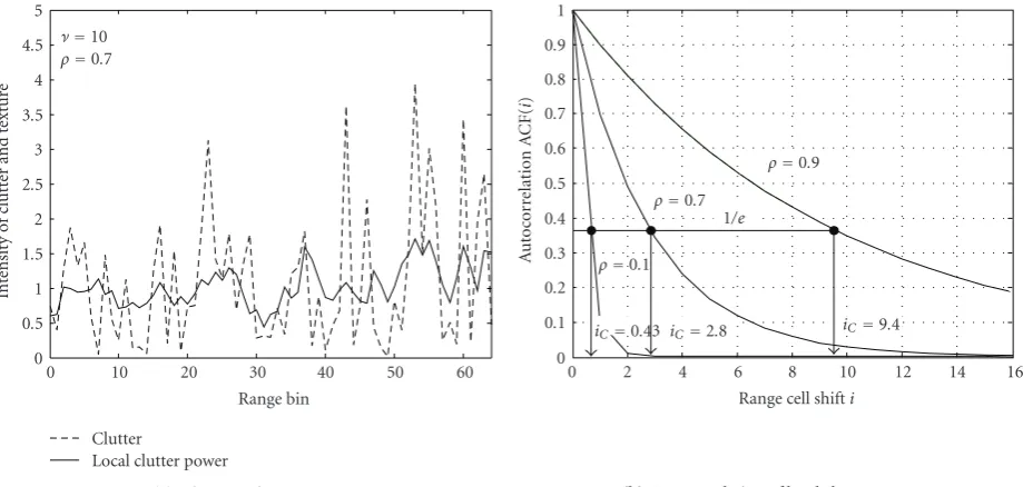
Figure 4 shows an example of the simulated clutter and the autocorrelation function of the local clutter power. In
Figure 4(a), the spatial clutter power fluctuation and strong clutter intensities (like as a spiky clutter) observed in range cells of 22, 44, and 53 are simulated. In Figure 4(b), the autocorrelation function withρ=0.1, 0.7, and 0.9 is shown and their correlation range cells are expressed by iC =
−1/lnρ, that is,iC = 0.43, 2.8, and 9.4, respectively. The
signal to clutter ratio denoted by SCR is defined as SCR =
τT/νθ, whereτT is the mean of the signal intensity (i.e., the
signal power). The threshold level is set to PFA = 10−4, and a total of 1×10⁶ independent Monte Carlo runs were performed.
3.1. Performance Characteristics. The hyperparameters, α0 and β0 in (6), should be given in accordance with the noninformative prior;α0 → 0 andβ0 → ∞. Howeverα0=1 andβ0 =0 are given as described inSection 2.2.2. Particu-larly, the value ofβ0 is in conflict with the noninformative prior. Therefore, the effect ofα0 andβ0on the probability of detection PD should be investigated.Figure 5shows the simulation results for the investigation, whereM=2 andν= ∞ (i.e., the exponential distributed clutter; homogeneous clutter), and the results of an ideal detector are also shown. The ideal detector is defined as the CA-CFAR with known local clutter power in the CUT; it provides the maximumPD. InFigure 5(a), whereβ0=0, it is found thatPDfor eachα0 is almost the same and is independent ofα0. InFigure 5(b), whereα0 =1, it is shown thatPDis improved by increasing β0. From these results, it is expected that the value of a larger β0gives a higherPD. However, in this study,β0=0 is chosen because of the analyticalPFAderivation.
Figure 6shows the effect of the number of reference cells MonPD, whereν= ∞andν=0.5 (heterogeneous clutter) are given. Figure 6(a) shows the result of the clutter with
ν = ∞. It can be seen thatPD generally increases withM and is close to thePDcurve for the ideal detector. From the PDfor the ideal detector, the CFAR loss [18] atM =2 and PD=0.5 is about 9 dB. Note that the loss of the CA-CFAR is more than 10 dB at the sameMandPD[2]. The CFAR loss of the proposed technique is found to be small. The accuracy of the estimated local clutter power is superior to the CA-CFAR and thePDis higher.Figure 6(b)shows the result for clutter withν = 0.5 and ρ = 0. The clutter distribution deviates considerably from the exponential and the condition of the local clutter power estimation is severe since the local clutter power is not correlated. It can also be seen thatPDincreases with M. From PD for the ideal detector, the CFAR loss at M = 2 andPD = 0.5 is about 20 dB. Compared with the homogeneous clutter shown inFigure 6(a),PDdecreases and the CFAR loss increases.
Figure 7 shows the effect of ν on PD, where M = 2, andρ = 0 and 0.9. In Figure 7(a) for clutter withρ = 0, PD increases with ν. It is worth remembering that the K distribution with a largeνis approximately the exponential (homogeneous) distribution. Thus, the proposed technique for homogeneous clutter provides higher PD than for the heterogeneous one. This phenomenon was also observed in the CA-CFAR [8]. Meanwhile inFigure 7(b), for clutter with ρ = 0.9,PDis almost the same for each value of νand is close to that forν = 10 in Figure 7(a). This is because the correlation length (iC=9.4 inFigure 4(b)) encompasses the
reference cells forM=2; thus, the local clutter power in the reference cells can be regarded as the same as that in the CUT.
0 5 10 15 20 25 30 35 40 SCR (dB)
0 0.1 0.2 0.3 0.4 0.5 0.6 0.7 0.8 0.9 1
PD
α0=1
α0=3
α0=10 Ideal (a) Effect ofα0;β0=0
0 5 10 15 20 25 30 35 40
SCR (dB) 0
0.1 0.2 0.3 0.4 0.5 0.6 0.7 0.8 0.9 1
PD
β0=0
β0=1
β0=3
β0=10 Ideal (b) Effect ofβ0;α0=1
Figure 5: Effect of hyperparameters on PD; M = 2, ν = ∞ (exponential distribution).
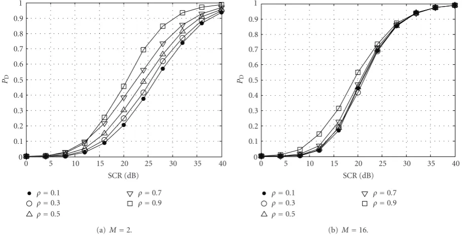
in the reference cell can be regarded as that in the CUT. Therefore, the accuracy of the local clutter power estimation is enhanced andPDbecomes high. InFigure 8(b)forM=16 (i.e., a large number of cells), the PD for ρ = 0.9 is the highest. Meanwhile,PD, except for ρ = 0.9, is almost the same because the values ofiCfor the clutter withρ=0.1 to
0.7, which areiC=0.43 to 2.8, respectively, are considerably
smaller than the number of reference cells. The local clutter power varies in the reference cells and the accuracy of the local clutter power estimation is then degraded.
Here, we consider guard cells effect on the performance. The spatial correlation between the local clutter power in the CUT and reference cells decreases with the increase of the
number of guard cells. From the results of the effect ofρas shown inFigure 8, therefore, the probability might depend on guard cells. For example, for a small number of reference cells,PDdecreases with the increase of number of guard cells as observed inFigure 8(a).
3.2. Performance Comparison. It may be interesting to make a comparison with conventional CFAR. Here, the CFAR techniques with the following local clutter power estimation methods of ML (i.e., conventional CA-CFAR), MAP, and MMSE (Bayes risk minimization) are considered.
The ML estimator is a simple method and no prior information of the local clutter power is needed. The local clutter power is estimated by
τML=arg max
τ L(τ|D)=Xm, (19)
where Xm = (1/M)
M
m=1Xm and Xm is the exponential
distribution conditioned on τ, defined by the right side in (5). The likelihood functionL(τ|D) in (19) is
L(τ|D)=
M
m=1
p(Xm|D). (20)
In the ML, the local clutter power is given by the mean of the reference data. When this estimator is used, the resulting detection structure is given by the well known CA-CFAR.
The MAP estimator depends on the details of the local clutter power distribution p(τ). Since the K distributed clutter is used in this simulation, the statistics of the local clutter power are then given as a Gamma distribution
p(τ)= 1
θMΓ(νM)τ
νM−1e−τ/θM, (21)
whereθM andνM are the scale and shape parameters. The
statistics of the speckle are the exponential conditioned onτ, that is, the local clutter power. The MAP estimator is found by maximizing a posterior distribution p(τ | D) ∝ L(τ |
D)p(τ). From the likelihood function in (20) and the prior distribution in (21), the result is
τMAP=arg max
τ p(τ|D)
=arg max
τ L(τ|D)p(τ)
= −1
2(M−νM+ 1)θM
+
1
4(M−νM+ 1) 2θ
M2+MXmθM.
(22)
The MMSE estimator also depends on the details of the local clutter power distributionp(τ), given as a Gamma dis-tribution. The estimated value by the MMSE is represented as [26]
τMMSE=
∞
0 τ p(τ|D)dτ
=
∞
0 τ
L(τ|D)p(τ)
∞
0 L(τ |D)p(τ)dτ dτ,
0 5 10 15 20 25 30 35 40 SCR (dB)
0 0.1 0.2 0.3 0.4 0.5 0.6 0.7 0.8 0.9 1
PD
M=2
M=8
M=16 Ideal
(a) Homogeneous clutter;ν=Inf (exponential distribution)
0 5 10 15 20 25 30 35 40
SCR (dB) 0
0.1 0.2 0.3 0.4 0.5 0.6 0.7 0.8 0.9 1
PD
M=2
M=8
M=16 Ideal (b) Heterogeneous clutter;ν=0.5,ρ=0 Figure6: Effect ofMonPD.
0 5 10 15 20 25 30 35 40
SCR (dB) 0
0.1 0.2 0.3 0.4 0.5 0.6 0.7 0.8 0.9 1
PD
ν=0.5 ν=1 ν=3
ν=5 ν=10 (a)ρ=0
0 5 10 15 20 25 30 35 40
SCR (dB) 0
0.1 0.2 0.3 0.4 0.5 0.6 0.7 0.8 0.9 1
PD
ν=0.5 ν=1 ν=3
ν=5 ν=10 (b)ρ=0.9 Figure7: Effect ofνonPD;M=2.
where p(τ | D) is the posterior distribution. Substituting the likelihood in (20) and the prior in (21) into (23), the estimated local clutter power is given by
τMMSE
=θMMXm·KM−νM−1
⎛ ⎝
4MXm
θM ⎞
⎠KM−ν
M
⎛ ⎝
4MXm
θM ⎞
⎠,
(24)
whereKp(x) is the modified Bessel function of second kind
of orderp.
In (22) and (24), the estimated local clutter powers,
τMAP and τMMSE, are the function of the parameters, θM
andνM. Thus, knowledge of these parameters is needed a
0 5 10 15 20 25 30 35 40 SCR (dB)
0 0.1 0.2 0.3 0.4 0.5 0.6 0.7 0.8 0.9 1
PD
ρ=0.1
ρ=0.3
ρ=0.5
ρ=0.7
ρ=0.9
(a)M=2.
0 5 10 15 20 25 30 35 40
SCR (dB) 0
0.1 0.2 0.3 0.4 0.5 0.6 0.7 0.8 0.9 1
PD
ρ=0.1
ρ=0.3
ρ=0.5
ρ=0.7
ρ=0.9
(b)M=16.
Figure8: Effect ofρonPD;ν=0.5.
known parameters, the probability of detection is higher than that in the conventional with estimated parameters. This is because, when using estimated parameters, the conventional method provides lower probability than with known parameters due to errors arising from the estimation. Therefore, in this comparison, these parameters are assumed as completely known and are set with the same values for the simulated sea clutter, that is,θM=θandνM=ν.
In the performance comparison, theKdistributed clutter withν=0.5, and the two with local clutter power spatial cor-relation,ρ=0.1 and 0.9, are used.Figure 9(a)compares the proposed detection method with the results of ML, MAP and MMSE estimator, whereM=2 and the clutter withρ=0.1. This provides a severe situation for the local clutter power estimation since the number of reference cells is small and the local clutter power fluctuates extremely. The proposed technique significantly outperforms the conventional ones. For example, at PD = 0.5, the SCR enhancement is 13 dB compared with MMSE.Figure 9(b)shows the performance comparison underM = 2 andρ = 0.9. This also provides the severe conditions; however, the local clutter power fluctuation is more moderate than in Figure 9(a). Again, the proposed technique outperforms the conventional ones.
Figure 9(c)shows the performance comparison underM =
16 andρ =0.1. In this condition, the number of reference cellsMis considerably large relative to the correlation range cell (iC = 0.43). The performance is almost the same, and
PD enhancement by the proposed should not be expected.
Figure 9(d) shows the comparison under M = 16 and ρ = 0.9. Similar to Figure 9(c), PD remains almost the same.
These results show that the proposed technique is supe-rior to CFAR with ML, MAP, and MMSE estimator, especially
when the number of reference cells is small and the local clutter power spatial correlation is weak.
4. Conclusions
In this paper, a CFAR detection technique in sea clutter for noncoherent radar systems was introduced, where heteroge-neous sea clutter is considered. The technique mainly applies the Bayesian theory for adaptive estimation of the local clutter power in the CUT. The technique achieves detection with no prior clutter information and has the CFAR property with respect to the clutter. We investigated the detection performance through Monte Carlo simulations where K distributed sea clutter with spatially correlated local clutter power was used. The following conclusions can be drawn from the simulation results.
(1) The detection performance of the proposed tech-nique depends on the number of reference cells, the sea clutter distribution, and the spatial correlation of the local clutter power. The probability of detection increases with the number of cells, the shape param-eter of the sea clutter, and the correlation.
(2) The proposed technique is found to be very useful compared with the conventional CFAR detector in which the shape and the scale parameters are known a priori, especially when the number of reference cells is small and the spatial correlation of the local clutter power is weak.
0 5 10 15 20 25 30 35 40 SCR (dB)
0 0.1 0.2 0.3 0.4 0.5 0.6 0.7 0.8 0.9 1
PD
(a)M=2 andρ=0.1
0 5 10 15 20 25 30 35 40
SCR (dB) 0
0.1 0.2 0.3 0.4 0.5 0.6 0.7 0.8 0.9 1
PD
(b)M=2 andρ=0.9
0 5 10 15 20 25 30 35 40
SCR (dB) 0
0.1 0.2 0.3 0.4 0.5 0.6 0.7 0.8 0.9 1
PD
Proposed ML
MAP MMSE (c)M=16 andρ=0.1
0 5 10 15 20 25 30 35 40
SCR (dB) 0
0.1 0.2 0.3 0.4 0.5 0.6 0.7 0.8 0.9 1
PD
Proposed ML
MAP MMSE (d)M=16 andρ=0.9 Figure9: Performance comparison;ν=0.5 (2/2, 1/2).
technique into a collision avoidance radar system for ships or pleasure boat safety navigation.
Appendix
We derive the false alarm rate PFA. X is thus the clutter. Here, we slightly modify (2), where both the numerator and denominator are divided by the true local clutter power,τ,
T=X/τ
τ/τ· (A.1)
When the CUT does not include the target signal, the probability density function (pdf) of X is the exponential distribution with τ of the mean. Thus the pdf of the numerator in (A.1) is the exponential with unit variance. Next we consider the pdf of the denominator. Since the pdf of τ is expressed as the inverse Gamma distribution,
as expressed in (9),τbelonging to this distribution can be expressed as
τ∼
⎛
⎝α1
m=1
ym2
⎞ ⎠
−1
, (A.2)
where α1 is the order parameter given in (7), and the distribution of ym is the noncorrelated complex Gaussian
distribution with zero mean and β1 of the variance. Here, (A.2) is further modified as
τ∼β1
⎛
⎝α1
m=1
|nm|2 ⎞ ⎠
−1
, (A.3)
where the pdf ofnm is the noncorrelated complex Gaussian
(8) into (A.3), the distribution of the numeratorτ/τ is given by τ τ ∼ 1 τ ⎧ ⎨ ⎩ M
m=1
Xm+X+β0
⎫ ⎬ ⎭ ⎛
⎝α1
m=1
|nm|2 ⎞ ⎠
−1
=Y1 Y2
, (A.4)
where
Y1= 1 τ ⎧ ⎨ ⎩ M
m=1
Xm+X+β0
⎫ ⎬
⎭, Y2=
α1
m=1
|nm|2. (A.5)
Sinceβ0 =0, andXmandXare the clutter, the distribution
ofY1 is the Chi-square distribution withM+ 1 degrees of freedom, denoted byχ2
M+1. Similarly, the distribution ofY2is given byχ2
α1. Here,Y1/Y2is slightly modified as
Y1 Y2 =
Y1/(M+ 1) Y2/α1 ·
M+ 1 α1
=z0×M + 1 α1
,
(A.6)
where
z0≡Y1/(M + 1) Y2/α1 .
(A.7)
Since the pdf ofz0is theFdistribution [27], the pdf ofz ≡ Y1/Y2(i.e., the denominator in (A.1)) is given by
p(z)dz= Γ(M+ 1 +α1)
Γ(M+ 1)Γ(α1)·
zM
(1 +z)M+1+α1dz, (A.8)
whereΓ(·) is the Gamma function. Therefore, the distribu-tion ofTis represented by
p(T)dT=(M+ 1)Γ(M+ 1 +α1)
Γ(α1) ·U(M
+ 2; 2−α1;T)dT, (A.9)
whereU(a;b;x) is the confluent hypergeometric function of the second kind [23], expressed by
U(a;b;x)= 1
Γ(a)
∞
0
ga−1
1 +ga+1−be
−xgdg. (A.10)
Finally,PFAas a function ofηis given by
PFA
η=
∞
η p(T)dT
=Γ(M+ 1 +α1)
Γ(α1) ·U
M+ 1; 1−α1;η
.
(A.11)
From (A.11),PFAis not a function of the statistical parameter τof the clutter.
Next, we derive the probability of detection,PD. Since the signal is assumed as the Swerling I model described in
Section 2.1, the random variable of the numerator in (A.1), that is,X/τ, is expressed as the exponential distribution with 1 +τT/τ of the mean, where τT is the mean of the signal
intensity (i.e., the signal power). On the other hand, the distribution of denominator in (A.1) is also given by (A.8). Similar to the derivation ofPFA, the distribution ofTis thus
p(T)dT= M+ 1
1 +τT/τ·
Γ(M+ 1 +α1)
Γ(α1)
·U
M+ 2; 2−α1; T 1 +τT/τ
dT.
(A.12)
Therefore,PDas a function ofη, is given by
PD
η=
η
0 p(T)dT
=Γ(M+1 +α1)Γ(M+1)
Γ(α1) ·U
M+1; 1−α1; η 1+τT/τ
.
(A.13)
In (A.13), it is found thatPDis a function ofM,α1, and τT/τ.
References
[1] E. Jakeman and P. N. Pusey, “A model for non-Gaussian sea echo,”IEEE Transactions on Antennas and Propagation, vol. 24, no. 6, pp. 806–818, 1976.
[2] V. G. Hansen and H. R. Ward, “Detection performance of the cell averaging LOG/CFAR receiver,”IEEE Transactions on Aerospace and Electronic Systems, vol. 8, no. 5, pp. 648–652, 1972.
[3] M. Sekine, T. Musha, Y. Tomita, and T. Irabu, “Suppression of Weibull distributed clutters using a cell-averaging log CFAR receiver,”IEEE Transactions on Aerospace and Electronic Systems, vol. 14, no. 5, pp. 823–826, 1978.
[4] V. Anastassopoulos, G. A. Lampropoulos, A. Drosopoulos, and M. Key, “High resolution radar clutter statistics,”IEEE Transactions on Aerospace and Electronic Systems, vol. 35, no. 1, pp. 43–60, 1999.
[5] S. Haykin, C. Krasnor, T. J. Nohara, B. W. Currie, and D. Hamburger, “A coherent dual-polarized radar for studying the ocean environment,”IEEE Transactions on Geoscience and Remote Sensing, vol. 29, no. 1, pp. 189–191, 1991.
[6] F. Gini, M. V. Greco, M. Diani, and L. Verrazzani, “Perfor-mance analysis of two adaptive radar detectors against non-Gaussian real sea clutter data,”IEEE Transactions on Aerospace and Electronic Systems, vol. 36, no. 4, pp. 1429–1439, 2000. [7] S. Watts, “Radar detection prediction in K-distributed sea
clutter and thermal noise,”IEEE Transactions on Aerospace and Electronic Systems, vol. 23, no. 1, pp. 40–45, 1987.
[8] S. Watts, “The performance of cell-averaging CFAR systems in sea clutter,” in Proceedings of the IEEE National Radar Conference, pp. 398–403, May 2000.
[9] S. Watts and K. D. Ward, “Spatial correlation inK-distributed sea clutter,”IEE Proceedings F, vol. 134, no. 6, pp. 526–532, 1987.
[10] K. J. Sangston, F. Gini, M. V. Greco, and A. Farina, “Structures for radar detection in compound Gaussian clutter,” IEEE Transactions on Aerospace and Electronic Systems, vol. 35, no. 2, pp. 445–458, 1999.
[12] R. J. A. Tough, K. D. Ward, and P. W. Shepherd, “The modelling and exploitation of spatial correlation in spiky sea clutter,” inProceedings of the 2nd European Radar Conference (EURAD ’05), pp. 5–8, Paris, France, October 2005.
[13] M. Weiss, “Analysis of some modified cell-averaging CFAR processors in multiple target situations,”IEEE Transactions on Aerospace and Electronic Systems, vol. 18, no. 1, pp. 102–114, 1982.
[14] E. Jay, J. P. Ovarlez, D. Declercq, and P. Duvaut, “BORD: Bayesian optimum radar detector,”Signal Processing, vol. 83, no. 6, pp. 1151–1162, 2003.
[15] K. J. Sangston and K. R. Gerlach, “Coherent detection of radar targets in a non-Gaussian background,”IEEE Transactions on Aerospace and Electronic Systems, vol. 30, no. 2, pp. 330–340, 1994.
[16] F. Gini, G. B. Giannakis, M. Greco, and G. T. Zhou, “Time-averaged subspace methods for radar clutter texture retrieval,” IEEE Transactions on Signal Processing, vol. 49, no. 9, pp. 1886– 1898, 2001.
[17] D. Gamerman, Markov Chain Monte Carlo: Stochastic Sim-ulation for Bayesian Inference, Chapman & Hall/CRC, Boca Raton, Fla, USA, 2002.
[18] M. I. Skolnik,Radar Handbook, McGraw-Hill, Boston, Mass, USA, 2nd edition, 1990.
[19] H. Watanabe, Introduction to Bayesian Statistics, Fukumura Press, 2003.
[20] N. Ueda, “Bayesian learning. [II]: introduction to Bayesian learning,”Journal of the IEICE, vol. 85, no. 6, pp. 421–426, 2002.
[21] C.-M. Cho and P. M. Djuri´c, “Detection and estimation of DOA’s of signals via Bayesian predictive densities,”IEEE Transactions on Signal Processing, vol. 42, no. 11, pp. 3051– 3060, 1994.
[22] P. M. Djuri´c and S. M. Kay, “Predictive probability as a criterion for model selection,” in Proceedings of the IEEE International Conference on Acoustics, Speech, and Signal Processing (ICASSP ’90), vol. 5, pp. 2415–2418, 1990. [23] L. C. Andrews,Special Functions of Mathematics for Engineers,
Oxford University Press, Oxford, UK, 2nd edition, 1998. [24] F. T. Ulaby, R. K. Moore, and A. K. Fung,Microwave Remote
Sensing: Active and Passive, Artech House, London, UK, 1986. [25] F. F.Gini and M.V. Greco, “Suboptimum approach to adaptive coherent radar detection in compound-Gaussian clutter,” IEEE Transactions on Aerospace and Electronic Systems, vol. 35, no. 3, pp. 1095–1104, 1999.