Research Article
A Feedback-Based Algorithm for Motion Analysis with
Application to Object Tracking
Shesha Shah and P. S. Sastry
Department of Electrical Engineering, Indian Institute of Science, Bangalore 560 012, India
Received 1 December 2005; Revised 30 July 2006; Accepted 14 October 2006
Recommended by Stefan Winkler
We present a motion detection algorithm which detects direction of motion at sufficient number of points and thus segregates the edge image into clusters of coherently moving points. Unlike most algorithms for motion analysis, we do not estimate magnitude of velocity vectors or obtain dense motion maps. The motivation is that motion direction information at a number of points seems to be sufficient to evoke perception of motion and hence should be useful in many image processing tasks requiring motion analysis. The algorithm essentially updates the motion at previous time using the current image frame as input in a dynamic fashion. One of the novel features of the algorithm is the use of some feedback mechanism for evidence segregation. This kind of motion analysis can identify regions in the image that are moving together coherently, and such information could be sufficient for many applications that utilize motion such as segmentation, compression, and tracking. We present an algorithm for tracking objects using our motion information to demonstrate the potential of this motion detection algorithm.
Copyright © 2007 Hindawi Publishing Corporation. All rights reserved.
1. INTRODUCTION
Motion analysis is an important step in understanding a se-quence of image frames. Most algorithms for motion anal-ysis [1,2] essentially perform motion detection on consec-utive image frames as input. One can broadly categorize them as correlation-based methods or gradient-based meth-ods. Correlation-based methods try to establish correspon-dences between object points across successive frames to es-timate motion. The main problems to be solved in this ap-proach are establishing point correspondences and obtain-ing reliable velocity estimates even though the correspon-dences may be noisy. Gradient-based methods compute ve-locity estimates by using spatial and temporal derivatives of image intensity function and mostly rely on the optic flow equation (OFE) [3] which relates the spatial and temporal derivatives of the intensity function under the assumption that intensities of moving object points do not change across successive frames. Methods that rely on solving OFE ob-tain 2D velocity vectors (relative to the camera) while those based on tracking corresponding points can, in principle, ob-tain 3D motion. Normally, velocity estimates are obob-tained at a large number of points and they are often noisy. Hence, in many applications, one employs some postprocessing in the form of model-based smoothing of velocity estimates
to find regions of coherent motion that correspond to ob-jects. (See [4] for an interesting account of how local and global methods can be combined for obtaining velocity flow field.) While the two approaches mentioned above represent broad categories, there are a number of methods for obtain-ing motion information as needed in different applications [5].
One of the main motivations for us is that simple motion information is adequate for perceiving movement at a level of detail sufficient in many applications. Human abilities at perceiving motion are remarkably robust. Much psychophys-ical evidence exists to show that sparse stimuli of a few mov-ing points (with groups of points exhibitmov-ing appropriate co-herent movement) are sufficient to evoke recognition of spe-cific types of motion. (See [6] and references therein.) Our method of motion analysis consists of a distributed network of units with each unit being essentially a motion direction detector. The idea is to continuously keep detecting motion directions at a few interesting points (e.g., edge points) based on accumulated evidence. It is for this reason that we formu-late the model as a dynamical system that updates motion in-formation (rather than viewing motion perception as finding differences between successive frames). Cells tuned to detect-ing motion directions at different points are present in the cortex, and the computations needed by our method are all very simple. Thus, though we will not be discussing any bio-logical relevance of the method here, algorithms such as this, are plausible for neural implementation. The output of the model (in time) would capture coherent motion of groups of interesting points. We illustrate the effectiveness of such motion perception by showing that this motion information is good enough in one application, namely, tracking moving objects.
Another novel feature of our algorithm is that it incor-porates some feedback in the motion update scheme, and the motivation for this comes from our earlier work on un-derstanding role of feedback (in the early part of the signal processing pathway) in our sensory perception [7]. In the mammalian brain, there are massive feedback pathways be-tween the primary cortical areas and the corresponding tha-lamic centers in the sensory modalities of vision, hearing, and touch [8]. The role played by these is still largely unclear though there are a number of hypotheses regarding them. (See [9] and references therein.) We have earlier proposed [9] a general hypothesis regarding the role of such feedback and suggested that the feedback essentially aids in segregating evidence (in the input) so as to enable an array of detectors to come to a consistent perceptual interpretation. We have also developed a line detection algorithm incorporating such feedback which performs well especially when there are many closely spaced lines of different orientations [10,11]. Many neurobiological experimental results suggest that such corti-cothalamic feedback is an integral part of motion detection circuitry as well [12–14]. A novel feature of the method we present here is that our motion update scheme incorporates such feedback. This feedback helps our network to maintain multiple hypotheses regarding motion directions at a point if there is independent evidence for the same in the input (e.g., when two moving objects cross each other).
Detection of 2D motion has diverse applications in video processing, surveillance, and compression [2,5,15,16]. In many such applications, one may not need full velocity in-formation. If we can reliably estimate direction of motion for sufficient number of object points, then we can easily identify sets of points moving together coherently. Detection of such
coherent motion is enough for many applications. In such cases, from an image processing point of view, our method is attractive because it is simpler to estimate motion direc-tion than to obtain dense velocity map. We illustrate the use-fulness of our feedback-based motion detection for tracking moving objects in a video. (A preliminary version of some of these results was presented in [17].)
The main goal of this paper is to present a method of tion detection based on a distributed network of simple mo-tion direcmo-tion detectors. The algorithm is conceptually sim-ple and is based on updating the current motion information based on the next input frame. We show through empirical studies that the method delivers good motion information. We also show that the motion directions computed are rea-sonably accurate and that this motion information is useful by presenting a method for tracking moving objects based on such motion direction information.
The rest of the paper is organized as follows.Section 2 de-scribes our motion detection algorithm. We present results obtained with our motion detector on both real and syn-thetic image sequences in Section 3. We then demonstrate the usefulness of our motion direction detector for object tracking application in Section 4. Section 5 concludes this paper with a summary and a discussion.
2. A FEEDBACK-BASED ALGORITHM FOR MOTION DIRECTION DETECTION
The basic idea behind our algorithm is as follows. Consider detection of motion direction at a point X in the image frame. If we have detected in the previous time step that many points to the left ofXare moving towardX, and ifXis a possible object point in the current frame, then it is reason-able to assume that the part of a moving object, which was to the left ofXearlier, is now atX. Generalizing this idea, any point can signal motion in a given direction if it is a possible object point in the current frame and if sufficient number of points “behind” it have signaled motion in the appropriate direction earlier. Based on this intuition, we present a coop-erative dynamical system whose states represent the current motion. Our dynamical system updates motion information at timetinto motion at timet+ 1 using the image frame at timet+ 1, as input.
Our dynamical system is represented by an array of mo-tion detectors. States of these momo-tion detectors indicate di-rections of motion (or no-motion). Here we consider eight quantized motion directions separated by angleπ/4 as shown in Figure 1(a). So, we have eight binary motion detectors at each point in the image array.1 As explained earlier, we should consider only object points for motion detection. In our implementation we do so by giving high weightage to edge points.
In this system we want that a detector at timetsignals motion if it is at an object point in the current frame and it
1If none of the motion direction detectors at a pixel is ON, then it
0 1 2
3 5
6 7
4
(a) Motion direction 1
Motion direction 2
Excitatory support for Direction 2
Excitatory support for Direction 1
(b)
Figure1: (a) Quantized motion directions separated by anglepi/4, (b) direction 1 neighborhood in “up” direction, direction 2 neigh-borhood in “shown angled” direction.
receives sufficient support from detected motion of nearby points at timet−1. This support is gathered from a direc-tional neighborhood. LetNk(i,j) denote a local directional
neighborhood at (i,j) in directionk.Figure 1(b)shows di-rectional neighborhood at a point for two different direc-tions.
Let St(i,j,k) represent state of the motion detector
(i,j,k) at timet. The motion detector (i,j,k) is for signaling motion at pixel (i,j) in directionk. Every time a new image frame arrives, we update the system state. We develop the full algorithm through three stages to make the intuition behind the algorithm clear. To start with, we can turn on a detector if it is a possible object point in the current frame and if it receives sufficient support from its neighborhood about the presence of motion at previous time. Hence, for every new image frame we do edge detection and then update system states using
St+1(i,j,k)=φ
A
(m,n)∈Nk(i,j)
St(m,n,k) +BE(i,j)−τ
,
(1)
where A and B are weight parameters, τ is a threshold,
Nk(i,j) is the local directional neighborhood at (i,j) in the
directionk, and
φ(x)= ⎧ ⎨ ⎩
1 ifx >0,
0 ifx≤0. (2)
The output of an edge detector (at timet+ 1) at pixel (i,j) is denoted byE(i,j). That is,
E(i,j)= ⎧ ⎨ ⎩
1 if (i,j) is an edge point,
0 otherwise. (3)
As we can see in (1) the first term gives the support from a local neighborhood “behind (i,j) in directionk” at previ-ous time, and the second term gives high weightage to edge points. We need to choose values of free parametersAandB
and thresholdτ to ensure that only proper motion (and not noise) is propagated. (We discuss choice of parameter values inSection 3.1and the overall system is seen to be fairly robust with respect to these parameters.)
To make this a complete algorithm, we need initializa-tion. To start the algorithm, at t = 0, we need to initialize motion. To getS0(i,j,k), for alli,j,k, we run one iteration of Horn-Schunk OFE algorithm [3] at every point and then quantize the direction of motion vectors to one of the eight directions. We also need to initialize motion when a new moving object comes into frame for the first time. This can potentially happen at any time. Hence, in our current imple-mentation, at every instant, we (locally) run one iteration of OFE at a point if there is no motion in a 5×5 neighborhood of the point in the previous frame. Even though the quan-tized motion direction obtained from only one iteration of this local OFE algorithm could be noisy, this level of coarse initialization is generally sufficient for our dynamic update equation to propagate motion information fairly accurately.
This basic model can detect motion but has a problem when a line is moving in the direction of line orientation. Suppose a horizontal line is moving in direction→and then comes to halt. Due to the directional nature of our support for motion, all points on the line would be supporting mo-tion in direcmo-tion→at points to the right of them. This can result in sustained signaling of motion even after the line has stopped. Hence it is desirable that a point cannot sup-port motion in the direction of orientation of a line passing through that point. For this, we modify (1) as
St+1(i,j,k)
=φ
A
(m,n)∈Nk(i,j)
St(m,n,k) +BE(i,j)−CLk(i,j)−τ
,
A
B
C
X
Figure2: Disambiguating evidence for motion in multiple direc-tions (see text).
whereCis the line inhibition weight and
Lk(i,j)= ⎧ ⎪ ⎪ ⎨ ⎪ ⎪ ⎩
1 if line is present (in the image att+ 1) at (i,j) in directionk,
0 otherwise.
(5)
The line inhibition comes into effect only if the orientation of the line and the direction of motion are the same.
2.1. Feedback for evidence segregation
From (4), it is easy to see that we can signal motion in multi-ple directions. (I.e., at an (i,j),St(i,j,k) can be 1 for more
than one k.) In an image sequence with multiple moving objects, it is very much possible that they would be over-lapping or crossing sometime. However, since we dynami-cally propagate motion, there may be a problem of sustained (erroneous) detection of motion in multiple directions. One possible solution is to usewinner-take-all kind of strategy, where one selects direction with maximum support. But, in that case even if each direction has enough support, the cor-rect dicor-rection may be suppressed. Also, this cannot support detection of multiple directions when there is genuine mo-tion in multiple direcmo-tions. The way we want to handle this in our motion detector is by using a feedback mechanism for evidence segregation.
Consider making the decision regarding motion at a pointXat timetin the directions→and. SupposeA,B, andC are points that lie in the overlapping parts of the re-gions of support for directions→and, and suppose that at timet−1 motion is detected in both these directions atA,
BandC. (SeeFigure 2.) This detection of motion in multi-ple directions may be due to noise, in which case it should be suppressed, or genuine motion, in which case it should be sustained. As a result of the detected motion atA,B, andC,
Xmay show motion in both these directions irrespective of whether the multiple motion detected atA,B, andC is due to noise or genuine motion. Suppose that A,B, andC are each (separately) made to support only one of the directions atX. Then noisy detection, if any, is likely to be suppressed.
On the other hand, if there is genuine motion in both direc-tions, then there will be other points in the nonoverlapping parts of the directional neighborhood, so thatXwill detect motion in both directions. The task of feedback is to regu-late the evidence from the motion detected at previous time, such that any erroneous detection of motion in multiple di-rections is not propagated. In order to do this, we have inter-mediate outputSt(·,·,·) which we use to calculate feedback
and then binarizeSt(·,·,·) to obtainSt(·,·,·). The system
update equation now is
St+1(i,j,k)= f
A
(m,n)∈Nk(i,j)
St(m,n,k) FBt(m,n,k)
+BE(i,j)−CLk(i,j)−τ
,
(6)
where
f(x)= ⎧ ⎨ ⎩x
ifx >0,
0 ifx≤0. (7)
The feedback att, FBt(i,j,k), is a binary variable. It is
deter-mined as follows
if St
i,j,k∗−1 7
l=k∗
St(i,j,l)
> δSt
i,j,k∗,
then FBt
i,j,k∗=1, FBt(i,j,l)=0 ∀l=k∗
else
FBt(i,j,k)=1 ∀k,
(8)
where
k∗=arg max
l S
t(i,j,l). (9)
Then we binarizeSt+1(i,j,k) to obtainSt+1(i,j,k), that is,
St+1(i,j,k)=φ
St+1(i,j,k)
, (10)
whereφ(x) is defined as in (2). The parameterδin (8) de-termines the amount by which the strongest motion detector output should exceed the average at that point.
The above equations describe our dynamical system for motion direction detection. The state of the system attisSt.
This gives direction of motion at each point. This is to be up-dated using the next input image, which, by our notation, is the image frame att+ 1. This image is used to obtain the bi-nary variablesE andLkat each point. Note that these two
are also dependent on tthough the notation does not ex-plicitly show this. After obtaining these from the next image, the state is updated in two steps. First we computeSt+1 us-ing (6) and then binarize this as in (10) to obtainSt+1. The intermediate quantitySt+1 is used to compute the feedback signal FBt+1 which would be used in state updating in the next step. At the beginning the feedback signal is set to 1 at all points. Since our index,t, is essentially the frame num-ber, these computations go on for the length of the image sequence. At any point,t,Stgives the motion information as
(1)Initialization
•sett=0.
•Initialize motionS0(i,j,k) for alli,j,kusing optic flow estimates obtained after 1 iteration of Horn-Schunk method. •set FB0(i,j,k)=1, for alli,j,k.
(2) CalculateSt+1(i,j,k), for alli,j,kusing (6).
(3) Update FBt+1(i,j,k), for alli,j,kusing (8).
(4) CalculateSt+1(i,j,k), for alli,j,kusing (10).
(5) For those (i,j) with no-motion at any point in 5×5 neighborhood,
initialize the motion direction to that obtained with 1 iteration of Horn-Schunk method. (6) Sett=t+ 1 (which includes getting next frame and obtainingEandLkfor this frame); go to (2).
Algorithm1: Complete pseudocode for motion direction detection.
2.2. Behavior of the motion detection model
Our dynamical system for motion direction detection is rep-resented using (6). The first term in (6) gives the support from previous time. This is modulated by feedback to effect evidence segregation. The weighting parameterAdecides the total contribution of evidence from this part, in deciding a point to be in motion or not. The second term ensures that we give large weightage to edge (object) points. By choosing high value for parameterB, we primarily take edge points as possible moving points. The third term does not allow points on a line to contribute support to motion in the direction of their orientation. Generally we choose parameterCto be of the order ofB. In (6), parameterτwill decide the sufficiency of evidence for a motion detector. (See discussion at the be-ginning ofSection 3.1.) Every time a new image frame ar-rives, the algorithm updates direction of motion at different points in the image in a dynamic fashion.
The idea of using a cooperative network for motion de-tection is also suggested by Pallbo [18] who argues, from a biological perspective, that, for a motion detector, constant motion along a straight line should be a state of dynamic equilibrium. Our model is similar to his but with some sig-nificant differences. His algorithm is concerned only with showing that a dynamical system initialized only with noise can trigger recognition of uniform motion in a straight line. While using similar updates, we have made the method a proper motion detection algorithm by, for example, proper initialization, and so forth. The second and important diff er-ence in our model is the feedback mechanism. (No mecha-nism of this kind is found in the model in [18].)
In our model, the feedback regulates the input from pre-vious time as seen by the different motion detectors. The out-put of the detector at any time instant is thus dependent on the “feedback modulated” support it gets from its neighbor-hood. Consider a point (m,n) in the image which currently has some motion. It can provide support to all (i,j) such that (m,n) is in the proper neighborhood of (i,j). If currently (m,n) has motion only in one direction, then that is the di-rection supported by (m,n) at all such (i,j). However, either due to noise or due to genuine motion, if (m,n) currently has motion in more than one direction, then feedback be-comes effective. If one of the directions of motion at (m,n) is sufficiently dominant, then motion detectors in all other
di-rections at all (i,j) are not allowed to see (m,n). On the other hand, if, at present, there is not sufficient evidence to deter-mine the dominant direction, then (m,n) is allowed to pro-vide support for all directions for one more time step. This is what is done by (8) to compute the feedback signal. This idea of feedback is a particularization of a general hypothesis pre-sented in [9]. More discussion about how such feedback can result in evidence segregation while interpreting an image by arrays of feature detectors can be found in [9].
3. PERFORMANCE OF MOTION DIRECTION DETECTOR
3.1. Simulation results
In this section, we show that our model is able to capture the motion direction well for both real and synthetic image se-quences when the image sese-quences are obtained with a static camera. The free parameters in our algorithm are A,B,C,
δ, andτ. For current simulation for all video sequences, we have takenA=1,B=8,C =5,τ =10, andδ=0.7.2The directional neighborhood is of size 3×5.
By the nature of our update equations, the absolute val-ues of the parameters are not important. So, we can always takeAto be 1. Then the summation term on the right-hand side of (6) is simply the number of points in the directional neighborhood of (i,j) that contribute support for this mo-tion direcmo-tion. Suppose (i,j) is an edge point and the edge is not in directionk. Then the second term in the argument of
fcontributesBand the third term is zero. Now the value ofτ, which should always be higher thanB, determines the num-ber of points in the appropriate neighborhood that should support the motion for declaring motion in directionk at (i,j) (becauseA =1). WithB=8,τ =10, andA=1, we need at least three points to support motion. Since we want to give a lot of weightage to edge points, we keepB large. We keepCalso large but somewhat less thanB. This ensures that when (i,j) is an edge in directionk, we need a much larger number of points in the neighborhood to support the motion for declaring motion at (i,j). The values for the
2It is seen that the algorithm is fairly robust to the choice of parameters
(a) (b) (c)
(d) (e) (f)
Figure3: Video sequence of a table tennis player coming forward with his bat going down and ball going up at timet=2, 3, 4. (a)–(c) Image frames. (d)–(f) Edge output.
Figure4: Points in motion at timet=4 for video sequence inFigure 3.
parameters as given in the previous parameters are the ones fixed for all simulation results in this paper. However, we have seen that the method is very robust to these values, as long as we pay attention to the relative values as explained above.
Figures3(a)–3(c) show image frames for a table tennis sequence in which a man is moving toward left, the bat is going down, and the ball and table are going up. The corre-sponding edge output is given in Figures3(d)–3(f). In our
(a) (b) (c)
(d) (e) (f)
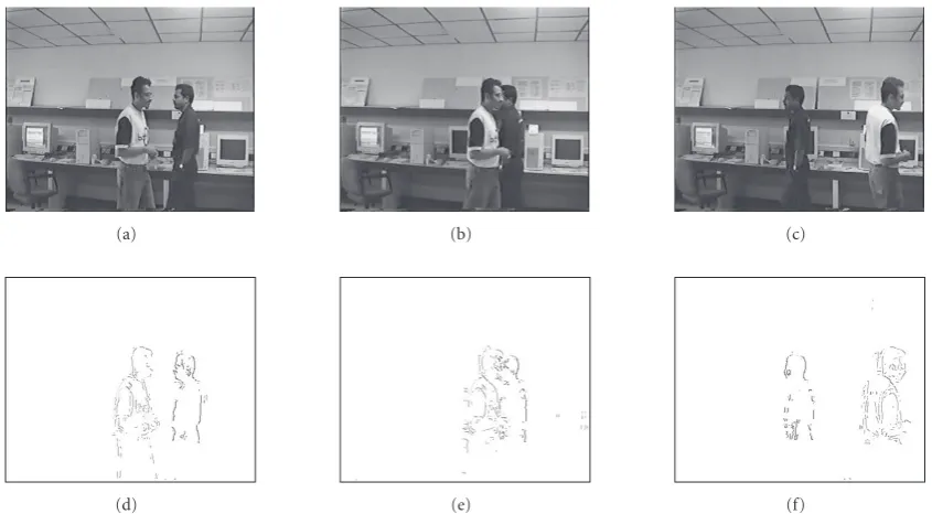
Figure5: Two men walk sequence (a) image frame at timet=6 (b) image frame at timet=12 (c) image frame at timet=35. Motion points in different gray values based on direction detected (d) at timet=6 (e) when the men are crossing, at timet=12, and (f) after the men crossed, at timet=35.
(a) (b) (c)
(d) (e) (f)
Figure6: Image sequence with three pedestrians walking on a road side. We show the image frames att=9, 19, 26, 37, 67, 80. Here we can see that they are walking in different directions and also cross each other at times.
Figure 5gives the details of the results obtained with our motion detector on another image sequence.3 Figures5(a),
5(b), and5(c)show image frames in a video sequence where two men are walking toward each other. Figures5(d),5(e), and 5(f) show edge points detected to be moving toward
3This video sequence was shot by a camcorder in our lab.
(a) (b) (c)
(d) (e) (f)
Figure7: Moving objects in the video sequence given inFigure 6. All the three pedestrians in the video sequence are well captured and different directions are shown in different gray levels. We can also see that the static background is correctly detected to be not moving. We show motion detected at (a) and (b) the beginning (c) and (d) while crossing each other (e) and (f) after temporary occlusion.
such information helps in properly segregating objects mov-ing in different directions even through occlusion like this. InFigure 5(b), at timet =12, we see that the two men are overlapping. Such occlusions, in general, represent difficult situations for any motion-based algorithm for correctly sep-arating the moving objects. In our dynamical system, motion is sustained by continuously following moving points. Note that motion directions are correctly detected after crossing as shown inFigure 5(f).
Figure 6shows a video sequence4where three pedestrians are walking in different directions and also cross each other at times.Figure 7shows our results for this video sequence. We get coherent motion for all three pedestrians and it is well captured even after occlusion as we can see inFigure 7(d).
Similar results are obtained for a synthetic image se-quence also. Figure 8(a) shows a few frames of a synthetic image sequence where two rectangles are crossing each other andFigure 8(b)shows the moving points detected. Our mo-tion detector captures momo-tion well and separates moving ob-jects. Notice that when the two rectangles cross each other there will be a few points with motion in multiple directions. Figure 8(c)shows the points with motion in multiple direc-tion. This information about such points can be useful for further high-level processing.
These examples illustrate that our method delivers good motion information. It is also seen that detection of only direction of motion is good enough to locate sets of points moving together coherently which constitute objects. To see
4It is downloaded fromhttp://www.irisa.fr/prive/chue/VideoSequences/
sourcePGM/.
the effect of our dynamical system model for motion direc-tion detecdirec-tion, we compare it with another modirec-tion direcdirec-tion detection method based on OFE. This method consists of running the Horn-Schunk algorithm for fixed number of it-erations (which is 15 here) and then quantizing the direc-tion of the resulting modirec-tion vectors into one of the eight directions. We compare motion detected by our algorithm with this OFE-based algorithm on hand sequence.5 (The video sequence is same as that in Figure 16.) Here a hand is moving from left to right and back again on a cluttered table.Figure 9shows the motion detected by our algorithm andFigure 10gives motion from the OFE-based detector. We can see that motion detected by our dynamic algorithm is more coherent and stable.
3.2. Discussion
We have presented an algorithm for motion analysis of an image sequence. Our method computes only direction of motion (without actually calculating motion vectors). This is represented by a distributed cooperative network whose nodes give the direction of motion at various points in the image. Our algorithm consists of updating motion directions at different points in a dynamic fashion every time a new im-age frame arrives. An interesting feature of our model is the use of a feedback mechanism. The algorithm is conceptually simple and we have shown through simulations that it per-forms well. Since we compute only direction of motion, the
5Available athttp://www.dai.ed.ac.uk/CVonline/LOCAL COPIES/ISARD1
(a)
(b)
(c)
Figure8: Synthetic image sequence with two rectangles crossing diagonally. (a) Image frames att =3, 10, 15. (b) Points in motion. (c) Points with multiple motion direction.
computations needed by the algorithms are simple. We have compared the computational time of this method versus an OFE-based method in simulations and have observed about 30% improvement in computational time [7].
As can be deduced from the model, there is a limit on the speed of moving objects that our algorithm can handle. The size of the directional neighborhood would primarily decide the speed that our model can handle. One can possibly ex-tend the model by adaptively changing the size of directional neighborhood.
In our algorithm (like in many other motion estima-tors), the detected motion would be stable and coherent mainly when the video is obtained from a static camera. However, when there is camera pan or zoom, or sharp change in illumination, and so forth, the performance may not be satisfactory. For example, when there is a pan or zoom almost all points in the image would show motion be-cause we are, after all, estimating motion relative to camera. However there would be some global structure to the de-tected motion directions along edges and that can be used to partially compensate for such effects. More discussion on this aspect can be found in [7]. For many video appli-cations, exact velocity field is unnecessary and expensive. The model presented here does only motion direction
de-tection. All the points showing motion in a direction can be viewed as points of objects moving in that(those) direc-tion(s). Thus the system achieves a coarse segmentation of moving objects. We will briefly discuss the relevance of such motion direction detector for various video applications in Section 5.
4. OBJECT TRACKER: AN APPLICATION OF THE MOTION DIRECTION DETECTOR
Tracking a moving object in a video is an important appli-cation of image sequence analysis. In most tracking applica-tions, a portion of an object of interest is marked in the first frame and we need to track its position through the sequence of images. If the object to be tracked can be modeled well so that its presence can be inferred by detecting some features in each frame, then we can look for objects with required features. Objects are represented either using boundary in-formation or region inin-formation.
(a) (b)
(c) (d)
(e) (f)
Figure9: Color-coded motion directions detected by our algorithm for hand sequence att=16, 29, 37, 53, 66, 78. (SeeFigure 16for the images.)
so forth. In [25], Blake and Isard establish a Bayesian frame-work for tracking curves in visual clutter, using a “factored sampling” algorithm. Prior probability densities can be de-fined over the curves and also their motions. These can be estimated from image sequences. Using observed images, a posterior distribution can be estimated which is used to make the tracking decision. The prior is a multimodal in general and only nonfunctional representation of it is available. The Condensation algorithm [25] uses factored sampling to eval-uate this. Similar sampling strategies are presented as devel-opments of Monte-Carlo method. Recently, various methods [25–27] based on this have attracted much interest as they of-fer a framework for dynamic-state estimation where the un-derlying probability density functions need not be Gaussian, and state and measurement equations can be nonlinear.
If the object of interest is highly articulated, then features-based trackingwould be good [22,28,29]. A simple approach to object tracking would be to compute a model to repre-sent the marked region and assume that object to be tracked would be located at place where we find the best match in the next frame. There are basically two steps in any feature-based tracking: (i) deciding about search area in next frame; and (ii) using some matching method to identify the best match. Motion analysis is useful in both the steps. Computational efficiency of such tracking may be improved by carefully se-lecting the search area which can be done using some motion
(a) (b)
(c) (d)
(e) (f)
Figure10: Color-coded motion directions detected by OFE-based algorithm for the hand sequence att=16, 29, 37, 53, 66, 78.
information. During the search for a matching region, also one can use motion along with other features.
(a) (b) (c)
(d) (e) (f)
Figure11: Tracking man 1 in video sequence given inFigure 6at timet=9, 19, 26, 37, 67, 80.
(a) (b) (c)
(d) (e) (f)
Figure12: Tracking man 2 in video sequence given inFigure 6at timet=9, 19, 26, 37, 67, 80.
In our tracking algorithm, we do not use any prior knowledge about the objects, their motion, or the camera pa-rameters. The only information provided (about the object) is a two-dimensional area selected (e.g., by the user) from first frame of the sequence. Thus here the term object refers to the marked portion that is being tracked. Our tracking al-gorithm has two steps: detection of motion directions, and matching of point sets.
our motion detection algorithm. Our motion detection al-gorithm segregates image region into clusters of coherently moving points. Object of interest would correspond to two such clusters in consecutive frames. So, we need to define matching method to compare two clusters to find the best match in a search area. We give two different matching meth-ods in the following two subsections.
4.1. Matching method 1: Hausdorff distance-based image comparison
Given two sets of pointsA= {ai},i=1,. . .,n, andB= {bj},
j=1,. . .,m, the Hausdorffdistance [30] is defined as
H(A,B)=maxh(A,B),h(B,A), (11) where
h(A,B)=max
a∈A minb∈Ba−b. (12)
The function h(A,B) is called the directed Hausdorff “distance” fromAtoB. Functionh(·,·) is not symmetric and thus is not a true distance. The Hausdorffdistance,H(A,B), measures the degree of mismatch between two sets, as it re-flects the distance of the point ofAthat is farthest from any point ofBand vice versa. Intuitively, if the Hausdorff dis-tance isd, then every point ofAmust be within a distance
dof some point ofBand vice versa. Here we use Hausdorff distance for comparing regions as follows. For matching we use only those object points that have motion. LetOmdenote
set of all points of objectOthat have motion. That is,
Om=xi,yi
|xi,yi
∈Oand we detect motion atxi,yi
in some directioni.
(13)
Then the distance between two objectsOandPis given by
HD(O,P)=HOm,Pm (14)
with · as Euclidean norm in (12).
4.2. Matching method 2: motion- and luminance-based distance
To measure similarity of regions in consecutive frames, here we define a simple distance measure based on motion and lu-minance information. Once the object of interest is marked by a window in the first frame, we represent it using a feature vector. First we divide the window into blocks of size 8×8 pixels. Suppose the window now containsM×Nblocks. Each block is assigned two parameters: one using motion and the other based on luminance. In every block if there are points with motion, then the motion feature is assigned the corre-sponding majority motion direction; else it is assigned no motion label. The other parameter to characterize each block is the average luminance of the pixels in that block. So, each block (m,n) is represented by Olum(m,n) and Omot(m,n),
m=1,. . .,Mandn=1,. . .,N. Here,Olum(m,n) would be a
real number andOmot(m,n) would be an integer in the range 0 to 8. When the value ofOmot(m,n) is in the range 0 to 7, it indicates the direction of motion as shown inFigure 1(a) while the value 8 indicates that there is no motion. Then to measure distance between two objectsOandP, we define
D(O,P)= m,n
αdOmot(m,n),Pmot(m,n)
+βOlum(m,n)−Plum(m,n), (15)
whereα =2,β =1; and we define difference in quantized motion direction,d(·,·), by the following 9×9 matrix given below. SinceOmot(m,n) takes an integer value between 0 and 8, this matrix completely specifies thed(·,·) function. The entries in the matrix are chosen based on ranking how far apart two quantized directions are:
d(i,j)= ⎡ ⎢ ⎢ ⎢ ⎢ ⎢ ⎢ ⎢ ⎢ ⎢ ⎢ ⎢ ⎢ ⎢ ⎢ ⎢ ⎢ ⎢ ⎢ ⎢ ⎣
0 1 2 1 4 2 4 6 8 1 0 1 2 2 4 6 4 8 2 1 0 4 1 6 4 2 8 1 2 4 0 6 1 2 4 8 4 2 1 6 0 4 2 1 8 2 4 6 1 4 0 1 2 8 4 6 4 2 2 1 0 1 8 6 4 2 4 1 2 1 0 8 8 8 8 8 8 8 8 8 0 ⎤ ⎥ ⎥ ⎥ ⎥ ⎥ ⎥ ⎥ ⎥ ⎥ ⎥ ⎥ ⎥ ⎥ ⎥ ⎥ ⎥ ⎥ ⎥ ⎥ ⎦ . (16)
4.3. Performance of tracking algorithm
In this section we present some simulation results of object tracking on a few video sequences. Note that the tracking is done without actually estimating any dense motion field. In all the results presented here, object to be tracked is se-lected in first frame by marking a window, and in subse-quent frames the results of tracking algorithms are shown by a window marked over the frame. We present results with the two different matching methods. We refer to these as Traker HD for the one using the method given inSection 4.1 and Traker D for the one using the method inSection 4.2. For these simulations, our motion detection algorithm uses the same parameter values as those used inSection 3.
For object tracking, first we give results with Track-er D. Figures11and12show results obtained on the video sequence shown in Figure 6. The square marked in Figure 11(a) is the object selected for tracking in the first frame. InFigure 11(c)we see that at timet=26 two people are crossing each other and occluding. Since our model sep-arates motion directions correctly and motion detection is by dynamically following moving points, we are able to track objects even during occlusions and when the view of the per-son changes. Similar results are obtained for tracking another man also in this video as shown inFigure 12.
(a) (b) (c)
(d) (e) (f)
Figure13: Results on tracking a full body (att=4, 6, 10, 14, 25, 35) in a video sequence where two men are crossing each other.
image frames in the video sequence and the result of tracking is marked by a rectangle. InFigure 13(d), at timet=14, we see that though the two men are overlapping, we are still able to track well. On the same video sequence,Figure 14shows that we can track a small portion of an object (the person’s hand) also well.
Figure 15gives results with Tracker HD on this two-men video sequence. This algorithm, which uses only motion in-formation, is also quite good at tracking. We show results of tracking the head of the man who is going behind the other man. Even though the object being tracked goes out of the video for a few frames, our dynamic motion detector is able to track it successfully and recapture the object after the oc-clusion. We can expect such performance from our method in general, if the object being tracked does not change its mo-tion through the occlusion.
Our next example is the hand sequence where a hand is moving on a cluttered table left to right and back, many times. Figures16and17show results on this hand sequence using Tracker D-based matching with only luminance infor-mation (i.e.,α=0,β=1) and both luminance and motion information (i.e.,α=2,β=1), respectively. We can see that we are able to track hand very closely inFigure 17with both luminance and motion information but not with just lumi-nance as can be seen in Figure 16. When the object is well separated from background, it is possible to track just based on luminance. But this result shows that just luminance alone is not sufficient to track object specially on such cluttered background. This video sequence is one by which the con-densation system [25] is tested and our results are well com-pared with those reported in [25].
From the results presented, it is reasonably well demon-strated that motion direction information at the edge points (as computed by our algorithm) is sufficient for application such as tracking moving objects.
5. CONCLUSIONS
In this paper we have presented a distributed algorithm that can detect and continuously update the direction of motion at many points, given a sequence of images. The model is a dynamical system whose state gives the motion directions at different points and the state is updated based on its cur-rent value and the next image. Thus the output of the model is a sequence of images containing direction of movement of some interesting points and thus captures groups of co-herently moving “feature” points. Perceptually, such moving point information seems to be good enough to evoke motion perception [6]. Thus, our model of a network that continu-ally keeps updating motion direction information could be a plausible model for routine motion perception.
(a) (b) (c)
(d) (e) (f)
Figure14: Results on tracking a hand (att=4, 6, 10, 14, 25, 35) in a video sequence where 2 men are crossing each other.
(a) (b) (c)
(d) (e) (f)
Figure15: Hausdorffdistance-based tracking for two-men-walk sequence (a) att=3, (b) att=6, (c) att=10, (d) att=14, (e) att=25 (after occlusion), and (f) att=35.
our algorithm can deliver seems to be adequate. For exam-ple, when a live teacher is being tracked (in a distance edu-cation set up), we would want to keep changing view such that teacher remains at the center of the frame. This can be very well be done with just motion direction-based tracking
as illustrated here. Similarly, the results of our tracker can be used to obtain rough trajectories of object motion which are useful, for example, in surveillance applications.
(a) (b) (c)
(d) (e) (f)
Figure16: Tracking a hand moving on a cluttered table with Tracker D using only luminance at timet=16, 29, 37, 53, 66, 78.
(a) (b) (c)
(d) (e) (f)
Figure17: Tracking a hand moving on a cluttered table with Tracker D using both luminance and motion at timet=16, 29, 37, 53, 66, 78.
points can directly give a coarse segmentation. One approach to object segmentation can be as follows. We can use a thresholding-based segmentation algorithm on each frame to oversegment the image in the sense that while an object may be broken down into many segments no segment con-tains more than one object. Then we can use the motion di-rection detection algorithm on the segment boundaries and, from this information, can infer which segments are coher-ently moving together and thus separate moving objects. In
our preliminary experiments, we had obtained promising re-sults with this technique. We would be exploring such appli-cations in our future work.
of motion. This could possibly be overcome to some extent by adding some time delays in the update equations of our nodes. Our method is essentially useful only when the cam-era is static because it can only detect 2D motion. For ex-ample, during a pan or zoom, the motion detected would be erroneous. However, changes in motion directions of objects would be distinctly different from those in apparent motion with camera zooms, pans, and so forth. By training a recog-nizer to classify types of motion based on the moving point patterns detected, it may be possible to detect and compen-sate for camera motion. We intend to address these issues also in our future work.
REFERENCES
[1] J. K. Aggarwal and N. Nandhakumar, “On the computation of motion from sequences of images: a review,”Proceedings of the IEEE, vol. 76, no. 8, pp. 917–935, 1988.
[2] C. Stiller and J. Konrad, “Estimating motion in image se-quences, a tutorial on modeling and computation of 2d mo-tion,”IEEE Signal Processing Magazine, vol. 16, no. 4, pp. 70– 91, 1999.
[3] B. K. P. Horn and B. G. Schunck, “Determining optic flow,” Artificial Intelligence, vol. 17, no. 1–3, pp. 185–203, 1981. [4] A. Bruhn, J. Weickert, and C. Schn¨orr, “Lucas/Kanade meets
Horn/Schunck: combining local and global optic flow meth-ods,”International Journal of Computer Vision, vol. 61, no. 3, pp. 211–231, 2005.
[5] R. J. Radke, S. Andra, O. Al-Kofahi, and B. Roysam, “Image change detection algorithms: a systematic survey,”IEEE Trans-actions on Image Processing, vol. 14, no. 3, pp. 294–307, 2005. [6] A. Casile and M. A. Giese, “Critical features for the recognition
of biological motion,”Journal of Vision, vol. 5, no. 4, pp. 348– 360, 2005.
[7] S. Shah,Feedback in low level vision: computional models and applications, Ph.D. thesis, Indian Institute of Science, Banga-lore, India, 2001.
[8] D. Mumford, “Thalamus,” inThe Handbook of Brain Theory and Neural Networks, M. A. Arbib, Ed., pp. 153–157, MIT Press, Cambridge, Mass, USA, 1995.
[9] P. S. Sastry, S. Shah, S. Singh, and K. P. Unnikrishnan, “Role of feedback in mammalian vision: a new hypothesis and a com-putational model,”Vision Research, vol. 39, no. 1, pp. 131–148, 1999.
[10] S. Shah, P. S. Sastry, and K. P. Unnikrishnan, “A feedback based algorithm for line detection,” inProceedings of Indian Conference on Computer Vision, Graphics and Image Processing (ICVGIP ’98), New Delhi, India, December 1998.
[11] S. Shah and P. S. Sastry, “Finger print classification using a feedback-based line detector,”IEEE Transactions on Systems, Man, and Cybernetics, Part B, vol. 34, no. 1, pp. 85–94, 2004. [12] E. H. Adelson and J. A. Movshon, “Phenomenal coherence of
moving visual patterns,”Nature, vol. 300, no. 5892, pp. 523– 525, 1982.
[13] M. S. Livingstone, “Mechanisms of direction selectivity in ma-caque v1,”Neuron, vol. 20, no. 3, pp. 509–526, 1998.
[14] L. Merabet, A. Desautels, K. Minville, and C. Casanova, “Mo-tion integra“Mo-tion in a thalamic visual nucleus,”Nature, vol. 396, no. 6708, pp. 265–268, 1998.
[15] W. Hu, T. Tan, L. Wang, and S. J. Maybank, “A survey on vi-sual surveillance of object motion and behaviors,”IEEE
Trans-actions on Systems, Man and Cybernetics, Part C, vol. 34, no. 3, pp. 334–352, 2004.
[16] A. Tekalp,Digital Video Processing, Prentice-Hall PTR, Engle-wood Cliffs, NJ, USA, 1995.
[17] S. Shah and P. S. Sastry, “Object tracking using motion direc-tion detecdirec-tion,” inProceedings of Indian Conference on Com-puter Vision, Graphics and Image Processing (ICVGIP ’00), Ban-galore, India, December 2000.
[18] R. Pallbo,Mind in motion, Ph.D. thesis, Lund University Cog-nitive Studies, Lund, Sweden, 1997.
[19] S. J. Dickinson, P. Jasiobedzki, G. Olofsson, and H. I. Chris-tensen, “Qualitative tracking of 3-d objects using active contour networks,” in Proceedings of IEEE Computer Soci-ety Conference on Computer Vision and Pattern Recognition (CVPR ’94), pp. 812–817, Seattle, Wash, USA, June 1994. [20] V. Caselles, R. Kimmel, and G. Sapiro, “Geodesic active
con-tours,” inProceedings of the 5th International Conference on Computer Vision (ICCV ’95), pp. 694–699, Cambridge, Mass, USA, June 1995.
[21] S. Kichenassamy, A. Kumar, P. Olver, A. Tannenbaum, and A. Yezzi, “Gradient flows and geometric active contour models,” inProceedings of the 5th International Conference on Computer Vision (ICCV ’95), pp. 810–815, Cambridge, Mass, USA, June 1995.
[22] B. Heisele, U. Kressel, and W. Ritter, “Tracking non-rigid, moving objects based on color cluster flow,” inProceedings of the IEEE Computer Society Conference on Computer Vision and Pattern Recognition (CVPR ’97), pp. 257–260, San Juan, Puerto Rico, USA, June 1997.
[23] N. Paragios and R. Deriche, “Geodesic active contours and level sets for the detection and tracking of moving objects,” IEEE Transactions on Pattern Analysis and Machine Intelligence, vol. 22, no. 3, pp. 266–280, 2000.
[24] M. Kim, J. G. Jeon, J. S. Kwak, M. H. Lee, and C. Ahn, “Mov-ing object segmentation in video sequences by user interaction and automatic object tracking,”Image and Vision Computing, vol. 19, no. 5, pp. 245–260, 2001.
[25] M. Isard and A. Blake, “Condensation—conditional density propagation for visual tracking,”International Journal of Com-puter Vision, vol. 29, no. 1, pp. 5–28, 1998.
[26] J. MacCormick and A. Blake, “A probabilistic exclusion prin-ciple for tracking multiple objects,”International Journal of Computer Vision, vol. 39, no. 1, pp. 57–71, 2000.
[27] C. Hue, J.-P. Le Cadre, and P. Perez, “A particle filter to track multiple objects,” inProceedings of IEEE Workshop on Multi-Object Tracking, pp. 61–68, Vancouver, BC, Canada, July 2001. [28] D. M. Gavrila and L. S. Davis, “3-d model-based tracking of humans in action: a multi-view approach,” inProceedings of IEEE Computer Society Conference on Computer Vision and Pattern Recognition (CVPR ’96), pp. 73–80, San Francisco, Calif, USA, June 1996.
[29] C. Bregler, “Learning and recognizing human dynamics in video sequences,” in Proceedings of IEEE Computer Soci-ety Conference on Computer Vision and Pattern Recognition (CVPR ’97), pp. 568–574, San Juan, Puerto Rico, USA, June 1997.
puter science from the Maharaja Sayajirao University of Baroda, 1992 and her Master’s and Ph.D. degrees in electrical engineering from Indian Institute of Science in 1996 and 2001, respectively. She has five years of ex-perience in industry research. She worked in areas of pattern recognition, computer vision, image processing, and data mining during her Ph.D. and continued
develop-ing real world applications for businesses in online search, mobile access-based search, and bioinformatics. Most recently at Yahoo!, she was with Applied Research Group as a Principle Research Sci-entist in Multimedia Group. Before that she worked at Strand Ge-nomics, Bangalore, with Data Mining Group as a Consultant.
P. S. Sastry received B.S. degree (honors) in physics from IIT, Kharagpur, in 1978, B.E. degree in electrical communications engineering, and Ph.D. degree from De-partment of Electrical Engineering, from IISc, Bangalore in 1981 and 1985, respec-tively. Currently he is a Professor in the Department of Electrical Engineering, In-dian Institute of Science, Bangalore. He has held visiting positions at University of