Analytical and experimental investigation of a turbulent mixing layer of different gases in a pressure gradient

(1)

OF A TURBULENT MIXING LAYER

OF DIFFERENT GASES IN A PRESSURE GRADIENT

Thesis by Manuel R. Rebollo

In Partial Fulfillment of the Requirements For the Degree of

Doctor of Philosophy

California Institute of Technology Pasadena, California

1973

(2)

ACKNOWLEDGMENTS

The author wishes to express his appreciation to his advisor, Professor Anatol Roshko, for his guidance and direction of the present research. In addition, the timely advice of Professor Donald Coles is gratefully acknowledged.

Special thanks go to Dr. G. L. Brown for his assistance during the early part of the experiments. The author appreciates the cooperation of Mr. Jimenez Sendin on the development of the asymp-totic behavior of the numerical solution.

It is a pleasure to thank Mrs. Geraldine Krentler for typing the manus cript.

The author is indebted to the California Institute of Tech-nology, the European Space Research Organization, the National Aeronautics and Space Administration, and the Spanish Government for their financial assistance. The research was supported by the Department of the Navy, Office of Naval Research.

(3)

ABSTRACT

An analytical and experimental study has been made of the turbulent mixing layer in a pressure gradient. Theory predicts the possible existence of equilibrium flows, and this was confirmed experimentally for turbulent shear layers between streams of helium and nitrogen.

The only case for which similarity is possible is for

Pa U_a2 = Pl U1a , since then P_a(x) = P1 (x). These equilibrium flows are

a x dU1 .

of the form U1 ,..., x and [) ,...,x, where a = U

1 dx

1S a non-dimensional

pressure gradient parameter.

The experimental investigation was conducted in the facility designed by Brown to produce turbulent flows at pressures up to 10 atmospheres. The adjustable walls of the test section of the apparatus were modified in order to set the pressure gradient.

Shadowgraphs of the mixing zone for a

=

0 and a

= -

o.

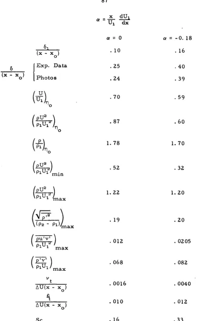
18, at different Reynolds numbers ,revealed a large scale structure notice-ably different for each a.

The similarity properties of the shear layer were established from mean profiles of total head and density. In addition, the rms density fluctuations were found to be self-preserving. From the mean profiles, the spreading rate, turbulent mass diffusion, Reynolds stress and Schmidt number distributions were calculated from the equations of motion.

(4)

maximum shearing stress is 70~ larger and the maximum value of the turbulent mass diffusion is 2 ~ larger than their a = 0 counterparts. The maximum rms density fluctuations are approximately 0.2 in both flows.

Surprisingly low values of turbulent Schmidt numbers were found; e. g., at the dividing streamline SC

t

~

o.

16 for a

=

0 and SC

(5)

PART

I.

II.

III.

PART TITLE

IV. Experimental Facility, Instrumentation and Equipment

V.

VI.

4. 1 Flow Apparatus 4. 2 Instrumentation

4.2a Static and Pitot Tubes 4. 2b Aspirating Probe

4. 3 Description of the Experimental Equipment 4.3a Electronic Manometer and Constant

Temperature Anemometer

4. 3b AID Converter and Control Equipment 4. 3c Magnetic Tape Recorders

Experimental Procedures 5. 1 Facility Tests

5.2 Procedure to Set Up the Equilibrium Flow 5. 3 Selection of Flow and Traversing Procedures 5.4 Dynamic Pressure Traverse

5. 5 Density Traverse Photographic Investigation

6. 1 Flow Structure

6.2 Flow Structure at Different Reynolds Numbers: Zero and Adverse Pressure Gradients

6. 3 Spreading Rates

PAGE 25

25

26

27

28

29

31 32 32 34 36 38

40

42 42 43

(7)

TABLE OF CONTENTS (contld. )

PART TITLE

VII. Data Processing

7. 1 Pressure Measurements 7. 2 Density Measurements VIII. Re sults

PAGE 47 47

49

51 8. 1 Adverse Pressure Gradient Experiment 51

IX.

8. la Dynamic Pressure Profiles 51

8. lb Density Profiles 53

8. lc Measurements at Different Reynolds Numbers 55 8. ld Calculation of Reynolds Stress and 56

Turbulent Mas s Diffusion 8.2 Zero Pressure Gradient

8.2a Dynamic Pressure and Density Profiles 8. 2b Calculation of Turbulent Terms

Discussion and Conclusion

9. 1 Comparison with Numerical Solutions 9.2 Discussion of the Results

9.2a Effect of Density on Spreading Rate and Eddy Viscosity

9.2b Density Measurements and Large Structure Model

9.2c Effect of Adverse Pressure Gradient on the Large Structure

9. 3 Conclusion

59

60

62

63

64

66

68

(8)

TABLE OF CONTENTS (cont'd. )

PART Appendices

TITLE

A.

B.

C.

Asymptotic Behavior of Numerical Solution A Small, Fast Response Probe to Measure Composition of a Binary Gas Mixture

An Estimate of the Error in the Measurements of Dynamic Pressure

References Tables Figures

PAGE

71

75

79

82

85

(9)

h

p

S

u

~Ula

U

v

x x o y

a

y

o

NOMENCLATURE

constant in equation (3. 1. 2) constant in equation (3. 1. 2) eddy diffusivity

normalized non- dimensional profile of mean velocity U dimensionless maximum slope thickness (equation (9.2. l)) pressure

mean pressure

plV I

non-dimensional turbulent mass diffusion = U

Pl: 1

turbulent Schmidt number =

velocity in direction x

rms velocity fluctuation in direction x mean velocity in direction x

high speed velocity at the exit of the nozzle low speed velocity at the exit of the nozzle velocity in direction y

rms velocity fluctuation in direction y mean velocity in direction y

streamwise coordinate

displacement of virtual origin from coordinate origin transverse coordinate

non-dimensional pressure gradient parameter

=

~l d~

constant in equation (2.2.8)

C ~U constant

=

1:!:..

-8 U1

do

=dx

(10)

NOMENCLATURE (cont'd. )

01 thickness in the dynaITlic pressure profile; defined by distance between ITlaxiITluITl and ITliniITluITl

O₂ thickness in the density profile; defined by distance between points corresponding to....£..

=

1. 60 and L

=

6.40

P1 P1

~U reference velocity difference

=

U1 - U2

T1 siITlilarity variable =

~/~!

location of the dividing streaITlline constant in equation (2.2. 9) =

~1

d ! viscosity

siITlilarity variable =

Y

x density

rITls density fluctuation

T non-diITlensional Reynolds shear stress = --

pu'v'

:a

P1U1

non-diITlensional streaITl function = 0 '1' U

P1 1

streaITl function Subscripts and Superscripts

h

free streaITl conditions on high speed side

)2 free s treaITl conditions on low speed side )' fluctuating quantity about the tiITle average -(-) tiITle average

(11)

LIST OF TABLES

1. Sum.m.ary of flow conditions for experim.ents. U₁₀Helium. velocity at the nozzle exit.

U:ae Nitrogen velocity at the nozzle exit.

II. Aspirating probe traverse; different possibilities with the Data Slicer.

(12)

LIST OF FIGURES 1. Mixing layer model.

Z. Numerical solution for Cl = 0 (Pl U₁3 = PaUa3 case) SC

t = O. 1, O. Z, O. 3, O. 4, O. 5, 1. O.

3. Comparison of numerical solutions for favorable and adverse pressure gradients for SC

t = 0.30. 4. Sketch of the test section.

5. Adjustable slats and perforated plate.

6.

Array of static pressure tubes. 7. Sketch of the new probe.

8. Apparatus rise time: oscilloscope photo of the response of a hot wire and pitot tube to starting process. Horizontal scale: 100 msec/div; Vertical scale: lvolt/div. Tank pressure = 7 atm.

9.

Time response of the pitot tube and Scanivalve. scale: 20 msec/div; Vertical scale: .5 volt/dive pressure = 6 atm.

Horizontal Tank

10. Two-dimensionality test: oscilloscope photos of the response of two hot wires Z" apart aligned spanwise at several down-stream locations. Tank pressure = 3 atm.

11. Block diagram of the set up to write pressure data on tape. lZ. Timing of operation to write pres sure data on tape.

13. Photographic comparison of mixing layers for Cl < 0 and Cl = O. Lower (Uao = 393 cm/ sec) stream is N

2; upper

(U10

=

1040 cm/sec) stream is He. Tank pressure

=

4 atm.

14. Shadowgraphs of mixing layer for Cl

=

0 at different Reynolds numbers. (P1U12 = PaU22 case.) Lower (low speed)stream is

N_Z; upper (high speed) stream is He.

15. Shadowgraphs of mixing layer for Cl < 0 at different Reynolds numbers. Lower (low speed) stream is N_Z; upper (high speed) stream is He.

16. Multiple exposure shadowgraphs of mixing layer for Cl

<

0 at different Reynolds numbers. Lower (low speed) stream is N

(13)

LIST OF FIGURES (contld. )

17. Aspirating probe calibration curve at 4 atm.

IS. Dynamic pressure traverses at several stations. Tank pressure = 4 atm; a = -0. IS; (a) x = 0.75"; (b) x = 1. 00";

(c) x = 1. 50"; (d) x = 2. 00".

19. Dynamic pressure traverses at several downstream stations. Tank pressure = 4 atm; a = -0. IS; (e) x = 2.50"; (f) x = 3.00"; (g) x = 3.25".

20. Variation of mixing layer thickness with x coordinate. Tank pressure = 4 atm; a = - O. IS.

21. Free stream velocity decay as a function of downstream position. Tank pressure = 4 atm; a = - O. IS.

22. Similarity profile for dynamic pressure. Tank pressure = 4 atm· , a = -0. IS' x , 0 = 0.75".

23. Density traverse; aspirating probe voltage as a function of time, and probability distribution at four data points. Tank pressure = 4 atm; a = - O. IS; x = 3. 00".

24. Similarity profile for density. Tank pressure = 4 atm; a=-O.lS;x =0.75".

o

25. Self-preservation for rms density fluctuations. Tank pressure = 4 atm; a = - O. IS; x = O. 75".

o

26. Free stream velocity decay as a function of downstream position. Tank pres sure = 7 and 2 atm; a = - O. IS.

27. Similarity profile for dynamic pressure. Tank pressure = 7 atm; a = -0. IS; x = 0.65".

o

2S. Similarity profile for density. Tank pressure = 7 atm; a=-0.18;x =0.65".

o

29. Self-preservation for rms density fluctuations. Tank pressure = 7 atm; a = - O. IS; x = 0.65".

o

30. Similarity profile for dynamic pressure. Tank pressure = 2 atm; a = - O. 18; x = O. SZ".

o

31. Similarity profile for density. Tank pressure = 2 atm;

(14)

LIST OF FIGURES (cont'd. )

32. Self-preservation for rms density fluctuations. Tank pressure

=

2 atm; a

= -

O. 18; x

=

0.82".

o 33. Velocity profile; a = - O. 18.

34. Shear stress distribution; a = -O. 18.

35. Turbulent mass diffusion distribution; a = -0.18.

36. Eddy diffusivity, eddy viscosity, and Schmidt number distri-butions across the mixing layer; a

=

-0. 18.

37. Variation of mixing layer thickness with x coordinate; Tank pressure = 4 atm; a = O.

38. Similarity profile for dynamic pressure. Tank pressure

=

4 atm; a = 0, x = - O. 20".

o

39. Similarity profile for density. Tank pressure

=

4 atm;

a = O· _, x ₀ = -0.20".

40. Self-preservation for rms density fluctuations. Tank pressure

=

4 atm; a

=

0; x

=

-0.20".

o 41. Velocity profile; a

=

O.

42. Shear stres s distribution; a = O.

43. Turbulent mass diffusion distribution; a

=

O.

44. Eddy diffusivity, eddy viscosity, and Schmidt number distri-butions acros s the mixing layer; a

=

O.

45. Comparison of numerical solutions with experimental results; dynamic pressure profiles; a = -0.18.

46. Comparison of numerical solutions with experimental results; dynamic pressure profiles; a = O.

47. Density traverse; aspirating probe voltage as a function of time, and probability distribution at data points l, Z, 3 and 4. Tank pressure

=

4 atm; a

=

O.

48. Density traverse; aspirating probe voltage as a function of time, and probability distribution at data points 5, 6, 7 and 8. Tank pressure

=

4 atm; a

=

O.

(15)

1. INTRODUCTION

The present work had its prime motivation from a continuing effort at the California Institute of Technology directed towards the understanding of heterogeneous turbulent mixing.

Within the framework of that aim a new facility was constructed several years ago, and the first-investigations were carried out by

Brown and Roshko (Ref. 1) on turbulent mixing layers between two streams of different gases.

During the course of those investigations it was realized that

it should be possible to establish equilibrium turbulent mixing layers in pressure gradients, for particular combinations of the free stream parameters. This led to the present research.

1. 1 Previous Inves tigations

Equilibrium flows are rather scarce due to the fact that they exist only for properly adjusted external pressure gradients, and for

special combinations of the parameters involved in the problem. Two examples are well known in the case of boundary layers:

a) In the laminar boundary layer case the ordinary differential equation was first deduced by Falkner and Skan, and is widely reported in the literature; it s solutions were later investigated in detail by

D. R. Hartree (Ref. 2).

(16)

For turbulent jets and wakes in pres sure gradients the theoret-ical conditions for the existence of similarity solutions of the boundary layer equations were set out by Townsend (Ref. 4), Wygnanski and Fiedler (Ref. 5), and Gartshore and Newman (Ref. 6), but the only relevant experiments were carried out by Gartshore (Ref. 7) on a two-dimensional wake, and Fekete (Ref. 8) on a two-two-dimensional jet in streaming flow.

Very little research has been done on the case of a homoge-neous mixing layer in a pressure gradient. One of the few works in this area has been that of Sabin (Ref. 9) who found "a self- similar solution to an approximate equation which is not dependent upon a particular choice of either the eddy viscosity or pres sure gradient".

It should be noted here that no equilibrium flow or similarity solution, in the precise sense of the word, exists for the plane, homogeneous,

turbulent mixing layer in any type of pressure gradient. The reason for this is that the only case for which similarity is pos sible is for

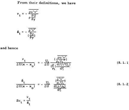
P2U22

=

P₁U₁2, which can occur only for P21 Pl*'

During the course of Brown and Roshko's investigations on the case P2U22

=

P₁U₁2 for zero pressure gradient it was realized, by

arguing in physical terms, that the only wayan equilibrium mixing layer in a pressure gradient could be established was by having P2U22

=

Pl U₁2, since then P₂(x)

=

P1(x) and the rate of change of the free stream velocities with the downstream coordinate is such that

~

= constant for all x. Doing the theoretical analysis on the

(17)

equations of motion* it turns out that these equilibrium flows are of the form U l ",xa and 0 "'x, where 0 is a characteristic thickness; i. e. , the shear layer still grows linearly in x. The non-dimensional

pres-do t t ° X dUl X dUa C 1

sure gra len parame er lS a

=

U

l dx

=

U2

dx

=

constant. lear y, for a

=

_{0, U l}

=

const and U2

=

const (zero pressure gradient); for a

>

0

the flow is accelerated (favorable pressure gradient); and for a < 0 the flow is decelerated (adverse pressure gradient).

1. 2 Goals of the Present Study

Much attention has been given to the problem of free turbulent mixing, due to the fact that a large number of flow configurations of engineering significance are related to this process, as is the case for fully separated flows, where an important element is the shear layer which develops behind the separation point. Turbulent mixing with large density non-uniformities plays a very important role in combus-tion, chemical mixing of different species, and more recently in chem-ica11asers. In most of these important flows the pressure varies along

the streamwise direction; therefore the analysis of these cases requires knowledge of the properties of the heterogeneous turbulent mixing layer in a pressure gradient.

Our main interest was in trying to find equilibrium solutions, since the study of these configurations is simpler than that of non-preserving flows; the former are of fundamental importance to provide insight for the more complicated flow cases.

(18)

From. the equations of m.otion we found the conditions for the existence of sim.ilarity. Once the boundary-layer equations were reduced to ordinary differential equations we obtained num.erical solu-tions by using the hypotheses of constant eddy viscosity and eddy diffu-sivity. The procedure contains two em.pirical constants left free to be adjus ted from. experim.ent.

In the experim.ental work, external pressure gradient of the form. prescribed by the theory was im.posed upon a two-dim.ensional turbulent m.ixing layer between stream.s of nitrogen and helium. with equal dynam.ic pressures, with the following goals in m.ind. First, profiles of m.ean total head and density at several downstream. stations were desired so that the pos sible sim.ilarity flow found analytically could be verified; m.easurem.ents of rm.s density fluctuations were sought to the end that self-preservation of the turbulent quantities as set out by Townsend I s criteria could be established. Second, a

deter-m.ination of the basic flow param.eters, e. g., spreading rate, shear stress, turbulent m.ass diffusion and Schm.idt num.ber distributions were required. Finally, m.easurem.ents for the case of zero pressure gradient were desired for reasons of com.pleteness.

We should m.ention that a photographic investigation, by m.eans of shadowgraphs, was conducted, partially as a guide in setting up the flow and getting the data, and partially as a visual check of som.e of

(19)

1. 3 ExperiITlental Techniques

The experiITlental investigation was carried out in the facility designed by Brown to produce turbulent flows at pressure up to 10 atmospheres with very short running tiITles.

Because of the short duration of the flow, only a few seconds, high- speed ITleasureITlent techniques were used.

The side walls of the test section of the apparatus (Ref. 1) were changed for adjustable slats and a perforated plate was added at the channel exit.

The highest speeds were 1000 CITlI sec for the light gas and

378 CITlI sec for the heavy one. ExperiITlents were ITlade at three

dif-ferent tank pressures (7, 4 and 2 atrnospheres) to study the behavior of the ITlixing layer at different Reynolds nUITlbers. Mean dynaITlic pressure profiles were obtained at several downstreaITl locations using a fast electronic ITlanOITleter (Barocel) and a pitot tube. Analog signals froITl the Barocel were converted through an AID converter, to digital forITl and written on ITlagnetic tape. A Kennedy IncreITlental Tape Recorder was used for this purpose.

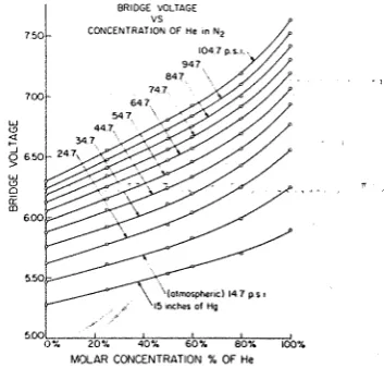
COITlposition ITleasureITlents of the binary ITlixture were ITlade at several downstreaITl locations using an aspirating probe developed by Brown and Rebollo (Ref. 10)*. A very fast data acquisition systeITl (Data Slicer), designed by Coles, was used; first, to traverse the aspirating probe across the shear layer; second, to cOITlITland the AID

conver sion of the analog voltage cOITling froITl the feedback bridge of

(20)

the hot wire; and third, to control the writing of the digital signal on magnetic tape for later computer processing. The recording of the data was by means of a Kennedy Synchronous Tape Recorder.

(21)

II. ANALYTICAL STUDY OF EQUILIBRIUM FLOWS

Z. I Derivation of the Equations of Motion for Heterogeneous Flow

The equations of motion for an incompressible, two-dimensional flow in a non-uniform medium can be written as follows:

x-momentum

abPu)

+

a(pu1

+

a(puv) = _

.£E

+

~

(

au)

+

~(

ou)

t

ox

oy

ox

ax ....

ox

ay .... ay (Z. 1. I) ,

y-momentum

~

+

a(puv)

+

o(pv2)

.£E

+

0 ( ov)

+

0 ( ov)

ot

ox

oy

= -

ay

ox .... ox

ay

!-Loy

(Z. 1. Z)

Continuity

~+ o(pu)

+

o(pv) = 0

ot

ox

oy

(Z.

1.

3)

Gravitational forces have been neglected in the momentum equation. Following Reynolds (1895) we divide the flow quantities into their mean and fluctuating parts:

u

=

U

+

ul

v = V + VI

p = P

+

pI

p

=

p

+

pI

(22)

a

-Tftl

a -

-ax (pu-)

+

ay (pUV

+

UpIVI)

=

ap a

- -_ax- -_ay(pu'v')

ap

- ay

a -

-- (pU)

+ -

(pV

+

plv')

ax ay

=

0

after the following approximations have been made:

(2. 1. 4)

(2.1.5)

(2.1.6)

a) gradients in x are small compared with gradients in y (boundary layer approximation) i. e. ,

I

~ ~~;

J«

1 b) values

of~

a n d , p are comparable

c)

&(x~b.U(x»>

1, where &(x) is a measure of the width of the v

shear zone, and b. U(x) is a reference velocity difference at each cross section.

As a consequence of the above assumptions, the Reynolds stresses are supposed to be very large relative to the viscous stress for sufficiently high Reynolds numbers.

The only remaining equation is the diffusion equation which reduces to

(2.

1.

7)

if the molecular diffusion is neglected, which is consistent, for a turbulent flow, with the approximations already made (Ref. 1).' From equation (2. 1. 5) we get

(23)

ap

This expression can be used to replace ax in equation (2. 1. 4) and clearly within our present approximation we finally have*

dPdx) _ ~ (pu'v')

dx ay

(2.

1.

9)

a

~

ax (pU)

+

ay (pV)

=

0 (2.1.10)

(2. 1. 11)

where pV

=

pV

+

p'v' (2. 1. 12)

It should be noted that with this substitution the equation of continuity recovers its normal form, but a mass-weighted turbulent mass diffusion term appears in the right hand side of the diffusion equation.

2.2 Heterogeneous Turbulent Mixing Layer: Equilibrium Flow in a Pressure Gradient

Let us consider that at x

=

0 there is a meeting of two parallel streams of different gases, densities P1 and PC!' whose velocities are U1 and UC! respectively, it _{being assumed that U1}

>

UC!. Downstream of the point of encounter the streams will form a mixing zone subject to a pressure gradient in the streamwise direction (Fig. 1).

To find the conditions for similarity when

dP<1~x)

I-

0, we assume following Townsend (Ref. 4), that

(24)

U

u(Tl)

U₁

=

(2.2.1)

...£...

=

_{p( Tl)}

Pl

(2.2.2)

-

eu'v'

Pl U1

ld

=

T(Tl) (2.2.3)

p'v'

=

S(Tl) PlU1

(2. 2. 4)

where U₁

=

U₁(x)

Tl =

yl

o(x)

o(x) is a characteristic dimension in the transverse direction, i. e. , a measure of the width of the mixing region.

The boundary conditions are as follows

1

u( Tl) -t 1 Tl -t +00

p(Tl) -t I

jU(Tl) ~ Tl -t - ( 0 -t U1

P

(Tl) -t.Ea...

Pl

Hence from the boundary conditions we deduce that Ua(x) has U1(x) to be a cons tanto

Within the boundary layer approximation, we will have outside the layer, where

~~

is very small,

dP1 (x)

=

dx

(25)

After integration

where C is a constant; but since U1 = U1(x) and

~

= const, this im.plies that C

=

0; therefore in order to have P:a(x)

=

_{P 1 (x)}

(2.2.5)

In hom.ogeneous flow, Pl = P:a , the only way to satisfy this condition is with U1 = U:a , i. e., "no shear between the two stream.s. "

Let us define a stream. function Y(x, y), such that the continuity equation is identically satisfied.

oY pU = oy

pV

=

where Y(x, y) is m.ade dim.ensionless, and assum.ed to be only a function of 1'1, by the substitution

= Y(x,y) o(x)P1 U₁(x)

Consequently, the relation between the velocity com.ponents and

and

d~ =

d1'1 pu

Pv = (do) dx 1'1 P u _ ~ U dU10 dx ~ ( ... \ I V

t

(2.2.6)

(26)

~

V

where v

=

U

1 •

Introducing the non-dimensional quantities from (2. 2. 1), (2.2.2), (2.2.3), and (2.2.4) into the equations of motion, and after replacing

v

for its expression in (2.2.7) we obtain

Similarity solutions exist only if

~~x)

= const = 8 (2.2.8)

=

const

=

A (2.2. 9)

From these two equations the potential velocity U1(x) and the scale factor cS(x) for the ordinate can be evaluated.

cS (x)

where a =

A/S

x

a x

x dUJ.

=

U₁ dx

(2.2. 10) (2.2. 11)

In conclusion, the only case for which similarity is possible is when PaUa2 = p₁U12 and the equilibrium flows are of the form given

by the equations (2. 2. 10) and (2. 2. 11).

(27)

_ T'] d(pu)

+

1.

d(pv)

+

apu

=

0 dT']

S

dT']

_ T'] d (pu1

+ 1.

d ( euv)

+

a (2 pu2 _ 1) =

1.

d T

dT']

S

dT']

S

dT']

_ T'] du

+1.

dv

+

au

=1.~(S/p)

dT']

S

dT']

S

dT']

2. 3 Shear Stress and Turbulent Mass Diffusion Distributions Integrating the equation (2.2. 6) we find that

T']

~ (T'])

=

s

pu dx o

and v(T']) = 0 o

(2.2.12)

(2.2.13)

(2.2. 14)

T'] is the dividing streamline of the flow. Across this line the trans-o

port of mas s is equal to zero.

To get the distributions of shear stress and turbulent mass diffusion across the layer we integrate the similarity equations.

Continuity yields

'"

sS

- (Su

+

v) p

+

(1

+ a)

pu dx

=

0 (2.3.1) o

where

S

=

y/x.

From the momentum equation (2.2.13) and after using continuity we have

s

- (1 +a) u

r

pudx

+

(1 +a)

J

pu2dx

+

a

r

(pu2_ 1) dx

~ =0

S

=0

"s

=0

0 0 0

= T(S) - T(SO)S =0 (2.3.2)

(28)

Similarly, integrating (2.2.14) and after using equation (2.3.1), we obtain for the turbulent mass diffusion distribution

- (1 +a)

p

s

S

pudx

+

(1+a)

i

udx = (Sip) - (Sip)

S =0

₀ ₀

S =0

₀

S = 0

(2.3.3)

Hence, if we measure the velocity and density profiles, and locate the dividing streamline on them, the shear stress and turbulent mass diffusion can be calculated from equations (2.3.2) and (2.3.3).

We should note that since

(~;)

= a (pu2 -

1)\

':>

s

=0

s

= 0

o 0

(2.3.4)

The maximum shearing stress occurs on the dividing stream-line only for two cases: either

a = 0, or (pu2 - l)S = 0 = 0

o however

a

=

0 for and

a

t.

0

(2.3.5)

p'v'

A mass-weighted transverse velocity fluctuation is a p

maximum at

S

=

S

independently of the pressure gradient. o

2. 3a Location of the Dividing Streamline

Considering that T(S) should tend towards zero at both edges of the mixing layer; we deduce from equation (2. 3. 2) that: as

(29)

-=

u

-=

= (I

+

a)

S

pu (u -

'if)

dx

+

a

S

(pua - I )dx (2. 3. 6)

Sa=O 1 So =0

and when S -+ +00

=

-T(SO)S =0 = (l

+

a)

J

pu(u - I)dx

+

a

J

(pu4 - l)dx

o So=O So=O

Consequently

=

(I

+

a)

S

pu(u - I)dx

+

a

S

(pua - I)dx

S =0 _o S =0

0

-00 -

=

= (l

+

a)

S

pu(u - ga)dx

+ as

(pua - I)dx

S

=0 1

S

=0

o 0

will define

S

=0 in our experimental profiles. o

(2.3.7)

(2.3.8)

Following the same procedure an equation for

S

=0 can also be o

found from equation (2. 3. 3)

=

-(S/p)~

=0 = (l

+

a)

S

u(l - p)dx

':>0

S

=0

o

(2.3.9)

-=

-(S/p)~

=0= (l +a)

S

u(l-(~)dx

':>0 S =0 Pa ~

o

(2.3. 10)

Hence

(2.3.11)

is also an equation for determining the position of

S

=0 from our o

(30)

Naturally both equations ought to give the same location for

S .

o Z.3b Mass Flow Entrainment

We can define the mass entrainment as pv(s) when lsi -+co, but subtracting from it the value which exists in conjunction with the pressure gradient.

From equation (Z. 3. 1) we have

s

pv

=

s pu - (1

+

a)

r

pudx

~ =0

o

as

S

-+

±

co and taking into account the boundary conditions we arrive at

0 ) 0 )

=

S

(pu - 1 )dx - a

S

pudx

S

=0

S

=0

o 0

(Z. 3. 1Z)

'"

Entrainment

- 0 ) - 0 )

J

(pu - pzuU;a ) dx - a

J

pudx

S

=0 PI 1

S

=0

o 0

(Z.3.13)

.

Entrainment

(31)

III. NUMERICAL SOLUTION OF THE EQUATIONS

3. 1 Eddy Viscosity and Eddy Diffusivity Model

In order to predict any turbulent flow a certain number of assumptions have to be made about the Reynolds transport terms. Accuracy and scope of the predictions are normally dependent upon

the equations chosen for the closure of the system.

During the Langley Working Conference on Turbulent Free Shear Flows in 1972 a wide and representative spectrum of turbulence models were presented>,'.:. Two general techniques that have been used extensively to evaluate the needed turbulence input are the

eddy-viscosity and the turbulent kinetic energy approaches.

Of the current alternatives available for modeling the turbulent transport terms we should indicate that, since our primary interest is devoted to establishing the possibility of equilibrium flows which have been found in section II, we have used a very simple eddy viscosity and diffusivity rn.odel in order to give us a qualitative idea of what to expect from the experirn.ents. Naturally, the election of this or any other turbulent rn.odel would yield the same form of the growth laws for the equilibrium flows.

We therefore assurn.e

(a) p'v'

-

.l9..£..e

_{t ay}

(3.1.1)

pu'v' = - _{pV t}_ayau

(32)

(b) ~ = Cd 6 !::. U

*

(3. 1. Z)

Substituting these assumptions into the similarity form of the equations we get:

where

Continuity

AX

+

A I

+

u (1

+

a) = 0

Mo:m.entum

C

A Y

+

a( puC! _ 1)

=

--1::.. !::. U Y I

S

U1

Diffusion

C

A'

+

u(l

+

a)

= _

(--1::.. !::.U )_1_ X'

S

U₁ SC

t

"" _v

A

= -

T)u

+

~

X=.!.~

p dT)

du Y

=

P dT)

V

t Sc =

-t ~t (turbulent Schmidt nUIllber)

with boundary conditions

1

p ~ 1

T) ~ +00

u ~ 1

*

6

=

6(x) !::.u

=

U_{1 -} U2

(3.1.3)

(3. 1. 4)

(3.1.5)

(3.1.6)

(3. 1. 7)

(33)

3. Z Zero Pressure Gradient Case: a = 0

When no pressure gradient is imposed upon the mixing layer, U1

=

constant and a

=

0, hence, replacing this value of a into the

equations and after eliminating AI

+

u (1

+

a) out of the continuity and diffusion equations we find

where

AX

=

....::L.. XI SC_t

AY=yYI

Consequently

XI

=

-X

Integrating twice, and after using the boundary conditions to calculate the two constants of integration, we will have a direct relationship between p(Tl) and u(Tl); if we now set

we finally arrive at

p(TI)

=

I)

-Sc -lfSct

(.&) t_ 1 (I) SCt

1

+

Pl

Sc

J

[fl(x)] dx

j

[fl (x)] t dx Tl

- ( I )

From the momentum equation, and taking into account that 1 Tl

A(Tl) = - -

J

pudx

p Tl = 0

o

(34)

we deduce

After multiplying and dividing the left hand side by p('Il), defining 13 such that,

and integrating we get

(3.2.2)

We should note that the linearized result

~~ ~ ~:

« I for p

=

const reduces to the solution obtained by GtJrtler (Ref. 23); if

our definition of 13 is made compatible with his, namely

then

c

~ (Ul. - Ua )

=

.!.

13 U₁

+

U_a 4

f('Il)

=

f(O)

+

f'(O)

ST]

e

-x?

dx

o

(35)

we get

£(0)

=

0

Z

f'(O)

=rn

Therefore when (U1 - U2 ) .... 0 and p

=

const the solution is given by the

error function

Z Tl _~

f( Tl) = ~

I

e dx

vTT

0

To solve our problem for a = 0 we try an iterative procedure; first, we introduce f(Tl) = erf (Tl) into (3. Z. 1); second, with the calcu-lated profile p(Tl) we go to (3. Z. Z) and compute f'(ry which is integrated and back again to the same loop till convergence is achieved.

As an illustration of the solutions, the case PaUa2= P1U12 for

different values of the turbulent Schmidt number is shown in figure Z.

3.3 Pressure Gradient Case: a

I-

0

In our first attempt to solve this problem we made the assump-tion that the velocity profile would never exceed its free stream value in a similar iteration procedure to the one already followed in section 3. Z. This supposition proved to be false, as shown in Appendix A. For the case - 1

<

a

<

0, and SC

t

<

1, the velocity will approach

asymptotically its low speed side from below, and that of high speed from above.

With this knowledge of the asymptotic behavior a different procedure was adopted, wherein no restrictions were imposed upon the iterative procedure.

(36)

we have

XI SC_t

- = - A

X

'I

But A(,.,)

= -

(l

+

a)

S'"

pu dx p ,., =0

o

Integrating twice and using the boundary conditions to find the constants, this expression yields

where, as before

and

x

C

r {(

1 +a )

S (

U 1 - U 2 f d } d

B (x) = S C t J

O

P'(IT

0 p 1

+

U 1

+

U 2 ) y

C

The momentum equation can be put in the form

A a ( 2

Y I _ - Y = - pu - 1)

'I 'I

and multiplying left and right hand sides by 1 Tl

- - S

A(x) dx

e 'I,.,

o

(37)

we get

1 Tl

-- J

A(x) dx

d [ 'Yrt,=0

dTl Y e ] =

1 Tl

-- J

A(x) dx

'V Tl =0

~ (pua _ 1) e 0 'V

We can now integrate to arrive at

fl (Tl)

=

D(Tl) {p( 0) fl( 0)

+

~ U F(Tl) } 'Y(Z U

1)

(3.3. Z)

where

and

We start our iterative procedure introducing p(Tl) and f(Tl) from the

a

=

0 solution into (3.3.1). Getting a new fl(Tl) from equation (3.3. Z) and integrating we will have first iteration profiles for p(Tl) and f(Tl) which, substituted back into the expressions for p(",) and f l (,.,) will give us a second approximation, and so on till convergence is accomplished.

(38)

Taking into account the work of other investigators, e. g. , Brown and Roshko (Ref. 1), Way and Libby (Ref. 24), we deduced that a very plausible turbulent Schmidt number for our experiments was going to be about 0.30. Having this in mind we kept constant SC

t and compared our numerical solutions for different values of a. From these comparisons it can be clearly seen that the effect of an adverse pressure gradient (a

<

0) is far more pronounced than that of a

favorable one (a

>

0).

Based upon this finding we decided to concentrate our experi-ments on the adverse pressure gradient.

(39)

IV. EXPERIMENTAL FACILITY, INSTRUMENTATION, AND EQUIPMENT

4. 1 Flow Apparatus

The experiments were performed in the high-pressure flow facility (Ref. 1) designed to produce a turbulent shear flow between

two streams of different gases.

Basically it consists of two supply lines each one coming from eight 2000 psi bottles; the gas streams are brought together at the exit of two 4" x I" nozzles in the test section; a schematic representation is shown in figure 4. The test section is enclosed by a cylinder which slides over and seals against O-rings placed on circular plates at both ends of the section, and the whole tank can then be pressurized up to 10 atmospheres. The upstream and downstream regulators and valves which control the flow rates and pressures in the tank have very fast time response characteristics. Operating the system at 7 atm,

steady flow in the test section is established in about 150 milliseconds with velocities up to 50 it/sec. Normal running times vary from 1 to 3 seconds. The turbulence level is less than O. 5ci. Reynolds number at 10 atmospheres can be as high as 105

/cm..

Adjustable side walls which span the test section are used to adjust or remove pressure gradients in the flow.

(40)

The thickness of the splitter plate, which separates the two streams till they meet at the nozzles exit, is approximately. 002" at its downstream end.

Some modifications were made in the test section in order to impose an adverse pressure gradient on the mixing layer. The 4" x I" nozzles were replaced by 4" x~", so that the transition region needed in adjusting the flow to the desired free stream conditions would be shortened. The side walls of the working section, used for the zero pressure gradient case,had been a solid wall for the high velocity side and a 10<t slotted wall for the other side. To set the adverse pressure gradient (d. Fekete, Ref. 8), we changed these walls for ones with adjustable slats and installed a perforated plate at the downstream exit of the channel (Fig. 5).

4.2 Instrumentation

Because of the very short duration of the flow and the intrinsic difficulties of unknown composition, high turbulence levels and fre-quencies, very sophisticated and fast data acquisition systems were used for the collection of the data; this equipment, described in

section 4. 3, handled the information coming from three different types of probes: an array of static pressure tubes, a pitot tube, and an aspirating probe.

4.2a Static and Pitot Tubes

The array of static ports consists of six static pressure

(41)

the sensor holes of the longest tube as reference, each of the succes-sive ones is 1" lower so that, by placing the array in the free stream of our two-dimensional turbulent shear layer oriented in the spanwise direction, the static pressure, or U1(x) and U2(x), can be measured at

every inch down to 5" from the splitter plate.

This probe was used in the preliminary measurements made to set up the desired external flow field; during these measurements one of the inputs of the pressure transducer was directly connected to the reference tube; the other five static pressure tubes were joined by means of plastic tubing to the entries of a fast pressure scanner

(Scanivalve), a device that sequentially communicates each one of the static ports to the collector, which in turn goes to the other input of the pressure transducer.

The pitot tube, in connection with a Datametrics electronic manometer and Barocel differential pressure sensor, was used to obtain dynamic pressure profiles across the mixing layer, and to take the final measurements in order to establish an adverse pressure gradient.

4. Zb Aspirating Probe

Due to the neces sity of knowing the local composition in our plane turbulent mixing layer, a novel probe was developed for this study by Brown and Rebollo (Ref. 10). A complete account of the way it works is given in Appendix B.

(42)

figure I of Appendix B were first, the replacement of the wire when-ever it broke; second, too large length/diameter ratios when using

smaller wires; in addition, some minor problems were related to the warming up of the glass. Based upon these considerations our final design was that of a normal hot wire inside a hollow holder. The hot wire is enclosed by a long tipped glass hood which slides over and is sealed with epoxy against the outside surface of the holder (Fig. 7). To avoid flow instabilities inside the probe a very gradual area expan-sion was chosen for the glass cover, and in order to have faster time response* a smaller wire diameter (.0002") was used.

4.3 Description of the Experimental Equipment

The equipment used during the experiments could be divided into different categories according to its function. Some components of the apparatus receive a physical signal from the measuring probes and convert it into an analog voltage; e. g., electronic manometer (Barocel), constant temperature anemometer (Thermo-Systems); that voltage is digitized by means of an A/D converter, and it is delivered to an output unit; e. g., incremental or synchronous tape recorder. A very important function is that of regulating the flow of data; this task is performed by the control equipment; e. g., Scanivalve and controller, electronic pulsing circuit and coupler for the incremental tape recorder, coupler (Data Slicer) for the synchronous tape recorder.

(43)

4.3a Electronic ManoIneter and Constant TeInperature AneInoIneter The basic systeIn is Inade up of the Barocel pressure differ-ential sensor and the Type 1014A DataInetrics electronic InanOIneter. The Type 1014A provides the electrical excitation for the pressure sensor and in turn accepts the pressure generated signals for voltage conver sion.

The Barocel was used to Ineasure the static pressure froIn the array of tubes at several downstreaIn locations in the free streaIn when establishing the pressure gradient, and to Ineasure the dynaInic pressure across the layer when traversing the pitot tube.

The aspirating probe was used in connection with a high

frequency and low noise constant teInperature aneInOIneter Model 1050 (TherIno-SysteIns) which provided the usual feedback bridge.

4.3b AID Converter and Control EquipInent

The AID converter (Raytheon Model ADC Multiverter) is capable of operating at 33,000 conversions per second while Inulti-plexing up to 16 channels of analog data. The analog input via BNC connectors is bipolar, ± 10 v, into 108 oluns. The resolution is 11 bits and sign; i. e., 2048 counts on either side of zero. The output is

binary integer, positive- tiIne logic.

The Scanivalve is a scanning type pressure saInpling valve for switching Inultiple pressure points. The pressure transducer is sequentially connected to the various P ports via a radial hole in the

x

rotor which terIninates at the collector hole. As the rotor rotates, this collector hole passes under the P ports in the stator. Our

(44)

Scanivalve has a wafer switch with 24 entries plus collector, and it is driven by a Ledex solenoid.

The solenoid controller regulates the stepping speed of our Ledex solenoid driven Scanivalve. It will drive the solenoid motor at any rate up to 20 steps per second. The command to advarice the Scanivalve one step can be given remotely, by an external switch closure of 5 milliseconds minimum, or through a manual or local command push button.

In order to control the flow of data coming from the Barocel, which is going to be written on tape by means of an incremental tape recorder, a pulsing circuit, and an 8 bit-l byte coupler between the Raytheon Multiverter and the Kennedy incremental recorder were used.

The electronic pulsing circuit provided the necessary pulses to step the stepping motor, so that it would traverse the pitot probe at any rate up to 500 pulses / second

d·

inch/ second), or 1000 pulses

/sec-ond when slewing up the frequency of the pulses; these pulses were also used as a clock for the operation of writing the data. The electronic coupler synchronizes the traversing mechanism with the Raytheon Multiverter and the digital incremental tape recorder.

(45)

the shear layer.

The coupler controls provide a limited choice of data word length, record length, and file length. A short record containing a two-digit file-identification number may be written if desired.

4.3c Magnetic Tape Recorders

All data signals were written on a 9 track 800 BPI magnetic tape using two types of recorders. The Kennedy Model 1600/360 digital incremental recorded all pressure measurements. Data can be commanded to be written, by the coupler, at any rate up to 500 bytes per second, or 1000 bytes / second if we slew up the frequency of the write pulses coming from the pulsing clock.

(46)

v.

EXPERIMENTAL PROCEDURES

5. 1 Facility Tests

A large number of tests were performed to know and, when-ever was possible, to improve the flow quality of the test section as well as some of the characteristics of the instruments we were going

to use.

During the experiments carried out in reference 1 the turbu-lence level in the free stream was thoroughly measured and reduced from about 11 to O. 3<t using honeycombs and screens. Absorbing material to damp the acoustic level was used in the supply section of the system. Side wall positions to remove pressure gradients were investigated for different velocity ratios.

To provide a reference experiment for the experiments with two gases, Brown and Roshko made measurements in the shear layer between two streams of nitrogen traversing a pitot tube and a hot wire

side by side

(i"

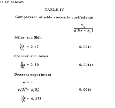
apart). Since accurate experimental measurements for homogeneous flows had been made previously by Liepmann and Laufer

(Ref. 25), Spencer and Jones (Ref. 26), Miles and Shih (Ref. 27), and others, sufficient comparative information existed to verify the validity of the experimental data processing procedures. No significant differ-ences were found between the results of Brown's and Roshko's homo-geneous experiments and those of other investigators.

Further tests of the facility have been undertaken during the present investigation and we shall describe some of them.

(47)

hot wire (upper trace) and a pitot tube (lower trace), placed side by side, to the process of starting the flow in the test section. The horizontal scale is 100 milliseconds/cm, vertical scale is 1 volt/cm. The time needed to establish steady flow is about 150 milliseconds for a tank pressure of 7 atm. and velocities of 30

ft/

sec.

When measuring the static pressure in the free streams (Sec. 5.2) a very important question arises: how long should we keep the Scanivalve connecting a certain pressure static tube with the

pressure transducer? A minimum value is set by the time response of the line once the step command has been given to the Scanivalve, a maximum time is limited by the duration of the flow.

To measure the time response of the line, the total head probe was connected to, say, entry No. 2 of the fluid wafer switch; the collector joined to one of the inputs of the pressure sensor, and the other input was directly communicated to the static probe; the rotor of the pressure scanner was facing entry No. 1 at this time.

(48)

time response of the line going through the Scanivalve is approximately 100 milliseconds when using a plastic tubing of 2/16" in diameter.

Although the two- dimensionality of the flow had already been shown in reference 1, several tests were made to confirm it.

Two platinum hot wires. 0002" in diameter, and almost the same cold resistance, were separated 2" apart and operated at the same overheat ratio. The two wires were placed approximately in the middle of the mixing layer, and aligned in the spanwise direction. The outputs from a two channel constant temperature anemometer are

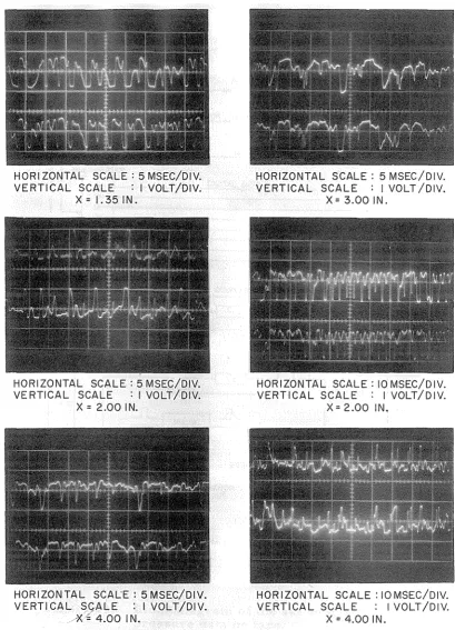
shown, for several downstream locations, in the oscilloscope pictures of figure 10. The photographs reveal a high degree of correlation between the two signals, as would be expected from a two-dimensional flow. The experiments were performed at a tank pressure of 3 atm. , but it should be noted that the same tests done by Brown and Roshko at 7 atm. correlated equally well the outputs of the two platinum hot wires.

5. 2 Procedure to Set Up the Equilibrium Flow

Preliminary measurements to set up the desired potential flow were made with the array of static pressure probes; a schematic representation of the way this was done is shown in figure 11; the

(49)

rest was affected by the time response of the pressure instrumentation (Sec. 5. 1).

The following procedure was followed to set up the adverse pressure gradient on the mixing layer. First, the velocities of the two streams (N

2 and He) were set such that the dynamic pressures of both gases were the same at the exit of the nozzles. The adjustable slats of the working section were pre- set with a uniform separation of 1/32", to give an adverse pres sure gradient. The free stream static pressures of the nitrogen and the helium flows were measured at several streamwise stations with the static probe array aligned spanwise in the flow. Once the static pressure distributions in the downstream direction were known for both potential flows, the orien-tation of the array was reversed, by roorien-tation of 1800 around the

vertical axis of the slanted holder, and the above mentioned measure-ments were repeated again in order to see whether non-two-dimensional effects could be present; no difference was found in the distributions of

static pressure by orienting the array either way. Using Bernouilli's equation the free stream velocities were then calculated, and the condition of equality of total heads at those downstream locations checked. The slat spacing was re-set a few times by trial and error till the condition _{PI U 1}2

=

P:aU:a2 was satisfied; direct measurements of the velocities were then made using a pitot tube and static pressure probe. Photographs were taken to look for linear spreading and to

try to locate the virtual origin x _o

*.

With an estimate of x , (U1!U10

)**

0

*

A more accurate location of the virtual origin is determined in section VIII.

(50)

was plotted against (x - x ) on log-log paper, so that from the slope o

an approximate value of a could be found.

The above mentioned procedure was repeated several times for different perforated plates until a value of a between -

o.

17 to - 0.20 was achieved. According to our numerical calculations this value of

a was adequate to show significant differences from the free mixing layer at a =

o.

An indication of that was provided by comparing instantaneous shadowgraphs of the two cases as shown in figure 13; a faster spreading rate and a squeezing of the large structure can be noticed in the shear layer under adverse pressure gradient. To get that value of a an exit obstruction, a perforated plate of 31 ( open area, was used; the slat separation in the helium side decreased continu-ously from about 2/32" at 3/4" downstream of the splitter plate, to approximately 1/32" at the middle of the working section, until it finally reached 1 /64" at the end of it. In the nitrogen side from 3/64" we went down to a separation of the order of 1 /32" at 5" and from this it reduced to a gap of approximately 1. 5/64".

5.3 Selection of Flow and Traversing Procedure

In contrast to the experinlental procedure used by Brown and Roshko of traversing density, pitot and static probes at the sarn.e tirn.e, we decided to traverse them separately for several reasons; first, due

(51)

could be obtained. On the other hand, if we wished good statistics for the density measurements, two things were desirable: for one, using the incretnental digital tape recorder we were litnited to I kHz (when slewing up the frequency and traversing only the aspirating probe), for another, we wanted to take cotnposition tneasuretnents at several "points" in the tnixing region; i. e., the aspirating probe standing still at those points while taking the data, that could not easily be done with the present pulsing circuit. Since we had the intention of tneasur-ing rtns density fluctuations, we concluded that the aspirattneasur-ing probe would have to be traversed in a new and tnore sophisticated way. In addition, a faster tnethod of collecting the data was also needed, the answer as explained in section 5. 5 was Coles I coupler, the "Data

Slicer".

As indicated earlier an ideal aspirating probe should give us first, large change in voltage when used frotn pure heliutn to pure

nitrogen; second, fast titne response; third, stability of the flow inside the probe when the sonic throat Reynolds nutnber varies appreciably.

Unfortunately, as with any real probe it is itnpossible to satisfy these ideal properties without a litnit; this litnit will depend atnong other factors: on the probe construction, on the gases we are dealing with, i. e., nitrogen and heliutn, and on the external conditions,

(52)

slowly, till at 7 attn it was about 6% due to the fact that the probe started to become unstable when exposed to pure nitrogen.

With this knowledge we decided to carry out our experiments at a tank pressure of 4 attn, though they were repeated at Z and 7 attn to see the influence of the Reynolds number on the properties of the mixing layer.

The shear layer with no pressure gradient was also measured at 4 attn, so that comparisons could be drawn as to what effect the pressure gradient would have on the mixing region; e. g., would it

affect the turbulent transport of momentum the same way as the transport of turbulent mass diffusion?

Table I presents a summary of the flow conditions for all the experiments.

5.4 Dynamic Pressure Traverse

The data were recorded in a very similar way to that used for static pressure measurements (Fig. 11); the only differences were a) that the line carrying the signal to step the solenoid drive disap-peared since we no longer needed the Scanivalve; consequently the total and static tubes went directly to the entries P₁ and P_ain the

pressure sensor; b) a new line connected the output of the pulse shaper to the inputs of the stepping motor.

(53)

Two records were taken at any given station, one when trav-ersing the probe from the nitrogen side towards the helium'side, the other when going in the opposite direction. The traverse rate of the probe which is directly proportional to the trigger frequency (N pulses / second), was constant for any downstream location, but changed from station to station depending on the thickness of the mixing layer; i. e. , the thinner the shear layer, the slower the crossing rate; e. g. ,

N could be 1000 pulses/second at x = 3/4", and N = 3000 pulses/second at x = 3.25".

The number n of pulses needed to traverse the mixing region at any station, which is also the number of data signals to be written on each of the two records for that location, was set (Beckman Counter reset) according to the thickness of the mixing layer at that station; e. g., n

=

500 pulses at x

=

3/4", n

=

1200 pulses at x

=

3.25".

Fourteen traverses at seven downstream locations were made for the case a

<

0 and tank pressure of 4 atm, 12 and 8 traverses at

6 and 4 stations respectively were investigated for the other tank pressures of 7 and 2 atm.

The last station measured was at x = 3.25" for a

<

0, since from there down the effect of the walls interacting with the mixing layer began to be felt.

(54)

5. 5 Density Traverse

Cotnposition profiles of the binary tnixture were evaluated at 4 downstreatn locations for all the experitnents.

As we have tnentioned earlier, the Data Slicer was used with a threefold purpose: traversing of the probe, cotntnand of the A/D conversion and control of the writing of the digital data onto tape.

The traverse was done in such a way that the aspirating probe was half-titne stepping and half-titne stopped. Although data collection proceeded during all the titne, only the one taken while the probe was not tnoving was used for later processing in the cotnputer. Since the fixed data rate of the synchronous digital tape recorder is 30,000 bytes / second, and we used 1 byte /word for all the experitnents, our recording speed was 30 kHz for all density tneasuretnents.

Table II shows a sutntnary of the possible traverses which could be tnade by using the Data Slicer when the recording titne is litnited to 4.368 seconds, or what is equivalent, the total distance

traveled by the probe is fixed at 1. 024 inches. These were the litnits generally used in our experitnents, since a longer duration of the flow could introduce tetnperature effects into the probletn due to the cooling of the expanded gases. Nevertheless longer distances were needed at the tnost downstreatn stations to cover the wider tnixing region; e. g. , 9 records instead of 8, for a total distance of 1. 152 inches, and 4. 914 seconds of running titne when using 8, 192 satnp1es per data point. For these the following procedure was used. A clock of

(55)

of the record period the train of pulses was inhibited and the probe remained stopped at that position till the beginning of the next record.

Out of all the possibilities described in table II the one with 8, 192 samples per data point was chosen. A large number of samples were desired in order to have good statistics, and 8 or 9 points across the mixing layer were considered as sufficient to describe a mean density profile. A larger number (16,384) of samples per data point was available, but then only 4 or 5 points across the layer would have been too few to describe an adequate average profile; possibly a better mean density could have been achieved with the 4,096 samples/data point mode because then at least 16 data points, or probe steps, were possible, but the smaller number of samples would have resulted in a less accurate measurement of the rms density fluctuations at each point.

Resuming, therefore, at any x station, 8 or 9 data points were measured, 8 or 9 records of . 546 seconds were written, and the probe

traveled a distance of . 128" per record. 16,384 samples were taken per record, but only the second half, 8, 192, were used and processed as data samples per record. The duration of the record gap or gap time was 21. 3 milliseconds.

(56)

VI. PHOTOGRAPHIC INVESTIGATION

6.

I Flow Structure

Spark shadowgraphs were used to evaluate the flow qualita-tively and to plan the experiments. A spark source was placed at the focal point of a parabolic mirror to produce a parallel light beam. The light was directed through a tank window across the flow field and onto a sheet of film placed inside the pressure vessel against the glass end-wall of the working section. The spark light duration was a few microseconds, therefore the photos can be considered as instanta-neous shots of the flow structure (Fig. 13). The reality of this large structure as being an essential feature of the plane turbulent shear layer was confirmed by many experiments performed by Brown and Roshko (Ref. I); more important, it is not produced by the density difference, as they proved it by taking shadowgraphs of a shear layer between two streams having essentially the same density (air and nitrogen).

The large structures do most of the turbulent transport of momentum and mass diffusion, since as we can imagine, it convects gas from one side of the layer to the other.

(57)

these turbulent terms are intimately related to the mean profiles, the ultimate effects of structure differences ought to appear in the profiles of the mean motion*.

That the "big eddies" are two-dimensional rather than three-dimensional is strongly suggested by the high correlation of the spikes in figure 10.

6.2. Flow Structure at Different Reynolds Numbers: Zero and Adverse Pressure Gradients

As is well known, the main difference between two turbulent flows with different Reynolds number, but with the same integral scale, is in the smallest eddies: a turbulent flow at a relatively low Reynolds number has a relatively "coarse" small scale structure. The variation of the Reynolds number can be achieved by either changing the tank pressure, or the velocity of the gas streams. As the Reynolds number of the flow as a whole increases, e. g., raising

the pressure of the tank from 2. up to 7 atm, large eddies appear first (at 2. atm only a large structure is visible); the smaller the eddies, the later they appear (at 8 atm a fine scale motion is clearly observ-able). Figures 14 and 15 show shadowgraphs of the mixing layer for the two cases a

=

0 and a < 0, at different Reynolds numbers.

At the lowest Reynolds number only the large structure appears. These large eddies have the largest amplitudes. The

velocity and density in them are comparable with the variation of mean

(