Schedulers
Thesis by Xiaoqi Ren
In Partial Fulfillment of the Requirements for the Degree of
Master of Science
California Institute of Technology Pasadena, California
2015
Acknowledgements
I am using this opportunity to express my deepest gratitude to my adviser, Prof. Adam Wierman. His excellent guidance, enthusiasm, patience and immense knowledge always inspires me and helps me overcome many obstacles during the past two years.
I am also grateful to my collaborators, Ganesh Ananthanarayanan, Minlan Yu and Michael Chien-Chun Hung. Their enormous help and constructive discussions are what made this thesis possible. The atmosphere and environment of the RSRG, Computer Science department and Caltech are amazing and helpful. It is really a pleasure to work and study here.
Abstract
Resource allocation and straggler mitigation (via “speculative” copies) are two key build-ing blocks for analytics frameworks. Today, the two solutions are largely decoupled from each other, losing the opportunities of joint optimization. Resource allocation across jobs assumes that each job runs a fixed set of tasks, ignoring their need to dynamically run speculative copies for stragglers. Consequently, straggler mitigation solutions are unsure of how to provide for speculative tasks. In this thesis, we proposeHopper, a new speculation-aware job scheduler. Hopperdynamically allocates resources for effective speculation based on theoretically derived guidelines that provably minimize average job completion time. In addition, Hopper also provides a simple knob for trading off fairness and performance. Evaluations on a 200-node cluster with Hadoop and Spark prototypes, on production work-loads from Facebook and Microsoft Bing, show job speedups of 50%−70% compared to SRPT schedulers, fairness schedulers, and straggler mitigation algorithms.1
Contents
Acknowledgements iii
Abstract iv
1 Introduction 1
2 Challenges and Opportunities 4
2.1 Background on Cluster Scheduling . . . 4
2.2 Strawman Approaches . . . 6
2.3 Speculation-aware Job Scheduling . . . 7
3 Scheduling Guidelines 9 3.1 Model design . . . 9
3.2 Model Features . . . 11
3.3 Virtual Job Sizes . . . 12
3.4 Dynamic Resource Allocation . . . 14
3.5 Incorporating Fairness . . . 19
4 Heterogeneous Job DAGs 26 4.1 DAG of Tasks . . . 26
5 Hopper: Design and Implementation 35
5.1 Data Locality . . . 35
5.2 Estimating Intermediate Data Sizes . . . 36
5.3 System Implementation . . . 37
6 Evaluation 38 6.1 Setup . . . 38
6.2 Hopper’s Improvements . . . 39
6.2.1 DAG of Tasks . . . 40
6.2.2 Speculation Algorithm . . . 41
6.3 Fairness . . . 42
6.4 EvaluatingHopper’s Design Decisions . . . 43
6.4.1 Locality . . . 44
6.4.2 Heterogeneous Stragglers . . . 45
6.4.3 Scheduler Scalability . . . 45
7 Related Work 47
Chapter 1
Introduction
In data analytics frameworks, application jobs are constructed as a DAG of phases with each phase running numerous parallel tasks (e.g., MapReduce [1], Dryad [2], Spark [3]). The tasks execute on compute slots over a large set of machines, and jobs are allocated slots for their tasks by the cluster-widejob scheduler.
Job scheduling is a much-studied topic, and there have been many algorithms suggested that seek to schedule the right jobs to run given the limited computing resources (slots) in order to minimize job completion time, e.g., [4, 5, 6, 7] or ensure fairness across jobs, e.g., [8, 9]. These algorithms take the requirements (number of slots) of the jobs when they arrive and allocate slots to them.
Unfortunately, in all prior work, job scheduling and straggler mitigation have been
decoupledfrom each other. Job schedulers assume that each job runs a fixed set of tasks and each task in the job requires a fixed amount of resources. However, given the existence of stragglers, each job may speculate new copies of tasks on the fly to speedup job completion. Straggler mitigation solutions, on the other hand, assume either a fixed amount of resources per job (which can be used for either speculation or scheduling new tasks), or a separate pool of resources that are reserved for speculative tasks.
While such decoupling was assumed for simplicity, it loses important analytical and systemic interactions, leading to significant inefficiencies. If the job scheduler performs best effort speculation by treating speculative tasks as normal ones, it often lacks the urgency required for speculative copies to be effective. However, if the scheduler budgets a fixed amount of resources for speculation, it risks reserving too little so as to not speculate enough tasks, or too much causing wastage of resources.
The main contribution of this thesis is the design of a newspeculation-aware job sched-uler that dynamically allocates resources to ensure effective speculation for each job. It does so to minimize the completion time of jobs. Our design is based on a theoretical model of schedulers built from first principles. Using this model, we derive structural (and simple) design guidelines forprovably optimal speculation-aware job scheduling.
In particular, based on the theoretical model, we introduce a virtual size for every job that includes the “optimal speculation level” for the job. The optimal speculation level is based on the job’s distribution of task durations and DAG characteristics. Building on virtual job sizes, we identify different resource allocation strategies based on the availabil-ity of slots in the cluster. When there are limited slots, we ensure the smaller jobs are allotted their virtual job sizes. When slots are sufficient, we allocate them proportionate to the virtual sizes of the jobs. Additionally, our theoretical model allows us to trade off performance for fairness using a simple knob.
sched-uler for cluster frameworks. To our best knowledge, Hopper is the first scheduler that integrates straggler mitigation with job scheduling for data analytics clusters. Hopperuses virtual sizes and the guidelines discussed above to schedule jobs, thus speculating smartly. In addition, Hopper incorporates many practical features of jobs into its scheduling. It estimates the amount ofintermediatedata produced by the job and pipelines their transfer between the job’s phases for better network utilization. It also carefully balances data locality requirements of tasks while staying faithful to the guidelines. Finally, Hopper is compatible with all existing straggler mitigation strategies (e.g., [13, 12, 14]).
To summarize, we make the following contributions:
1. We identify the importance of jointlydesigning job scheduling and straggler mitiga-tion in clusters.
2. Using a theoretical model from first principles, we develop structural scheduling guidelines foroptimal speculation-aware job scheduling.
3. We build a speculation-aware job scheduler,Hopperbased on the theoretical guidelines and generalize it to consider practical system constraints in clusters.
To evaluate the performance ofHopper, we have developed prototypes inside the Hadoop [15] and Spark [3] computing frameworks. In doing so, our objective is to demonstrate Hop-per’s generic design and also expose it to many varied factors in scheduling based on task durations, straggler causes and DAG patterns.
Chapter 2
Challenges and Opportunities
We now present the challenges and opportunities associated with joint decisions on job scheduling and straggler mitigation using simple examples and present some intuitions for joint scheduling decisions.
2.1 Background on Cluster Scheduling
We begin by describing the commonly used and relevant algorithms for job scheduling and straggler mitigation.
Job Scheduling: While job scheduling in clusters is a classical problem, traditional ap-proaches, typically, do not consider stragglers. They assume that each job has running time that is known a priori, and thus a job’s remaining duration can be estimated from the remaining durations of its running tasks and unscheduled tasks. Perhaps the two most studied job scheduling polices are the following: one aiming to minimize average job duration and the other focusing on fairness.
A3 A2
A1
time
B2
0 5 8
A1+ B3
B1
B1+ B5
B4
3 B6
A4 B2+
Slot 1 Slot 2 Slot 3 Slot 4 Slot 5 Slot 6
(a) SRPT: completion time for job A and B are 5 and 8.
3 0 6 B2 B1+ B4 8 A2 A1 A1+
A3 A4
B1 B6
B5
B3 time
Slot 1 Slot 2 Slot 3 Slot 4 Slot 5 Slot 6
(b) Fair: completion time for jobs A and B are 6 and 8.
Figure 2.1: Scheduling with “best effort” speculation for jobs A and B. The + suffix indicates a speculative copy.
A3 A2 A1
time B2
0 6 7
A1+ B3 B1 B1+ B4 3 A4 B2+ B5 B6 Slot 1 Slot 2 Slot 3 Slot 4 Slot 5 Slot 6
(a) SRPT: completion time for job A and B are 3 and 7.
B4 time 3 0 6 B2 8 B5 B6 B3 B1 A3 A2 A1 A4 A1+ B1+ B2+ Slot 1 Slot 2 Slot 3 Slot 4 Slot 5 Slot 6
(b) Fair: completion time for jobs A and B are 6 and 8.
Figure 2.2: Scheduling with “budgeted
speculation” (2 slots) for jobs A and B.
The + suffix indicates speculation.
server setting, although SRPT is no longer optimal in as strong a sense, it has the optimal achievable competitive ratio among online algorithms [4]. Of course, unfairness is a concern for SRPT given its prioritization of small jobs at the expense of large jobs.
Fair scheduling: Fairness is a crucial issue in many settings, and as a result, another popular job scheduler is based on fair allocations. Such schedulersfairlydivide the resources in the cluster (slots, memory, network etc.) among the jobs. Without loss of generality, we focus on the so-called Fair Scheduler, which is commonly used in cluster frameworks today (e.g., [8]). The Fair scheduler allocates the available compute slots evenly among all the active jobs. Such strong fairness naturally comes with performance inefficiencies compared to SRPT.
A3 A2 A1
time
Slot 1 Slot 2 Slot 3
B2
0 5 6
Slot 4 Slot 5 Slot 6
A1+ B3
B1 B1+
B4
3 A4 B5 B2+
B6
Figure 2.3: Hopper: completion time for jobs
A and B are 3 and 6, respectively.
!" !#" !$" !%" !&" '()('" *" %" %" %" ')+," $" $" $" $"
-" -#" -$" -%" -&" -." -/" '()('" /" /" %" %" #" #" ')+," $" $" $" $" #" #"
Table 2.1: tinit and tnew are task du-rations of the original and speculative
copies. trem = tinit – elapsed time.
capacity, decides when to schedule speculative copies of tasks. There are many varieties of speculation strategies, e.g., [13, 12, 14], which differ in their decisions of when to spawn speculative copies as well as how many speculative copies to spawn.
For simplicity, we assume the following speculation strategy: if the remaining running time (trem) is longer than the time to run a new task (tnew), speculate a new copy. We also assume that the straggler can be detected after a new task runs for a small amount of time.
2.2 Strawman Approaches
SRPT and Fair scheduling do not explicitly take into account speculation policies. We now explore two natural strawman approaches for them to consider speculative copies. We use the strawman approaches to highlight the fundamental difficulties that motivate the need for dynamic joint decisions of scheduling and speculation.
Best-effort Speculation: Perhaps the most simple approach is to just treat speculative tasks the same as normal tasks. Thus, the job scheduler allocates resources for speculative tasks in a “best effort” manner, i.e.,whenever there is an open slot. For example, for the SRPT policy that prioritizes the job with the shortest remaining time, a speculative copy for its task is scheduled when a new slot opens; crucially speculative copies are run only
when new slots become available.
Concretely, in Figure 2.1a, the SRPT job scheduler has to wait till time 3 to find an open slot for the speculative copy of A1.1 Clearly, this approach is problematic. For
1
example, in Figure 2.1a if the job scheduler had allocated resources to speculative tasks earlier, then job A’s completion time would have been reduced, without slowing down job B (see Table 2.1 for the task durations).
The problem is also present with Fair scheduling. In Figure 2.1b, where both jobs are allotted 3 slots, job A can only speculate task A1 when task A2 finishes. If it could have speculated earlier, job A’s completion time would have reduced, again, without slowing down job B.
Budgeted Speculation: An alternative approach is to have the job scheduler reserve a fixed “budget” of slots for speculative tasks. In this way, speculative tasks for stragglers do not have to wait and can be run much earlier, thus alleviating the issues discussed above. Budgeting the right size of the resource pool for speculation, however, is challenging because of varying straggler characteristics and fluctuating cluster utilizations. If the resource pool is too small, it may not be enough to immediately support all the tasks that need speculation. If the pool is too large, resource are left idle.
Concretely, in Figure 2.2a, two slots (Slot 5 and Slot 6) are reserved for speculative tasks. Slot 6 is vacant from time 0 to 3. If the job scheduler could have used the wasted resource to run a new task, say B1, then job B’s completion time would have been reduced. The problem is also present with Fair Scheduling. In Figure 2.2b, if the job scheduler could have used Slot 6 to run B4 at time 3, then job B’s completion time would have reduced.
Finally, note that reserving one instead of two slots will not solve the problem, since both SRPT and Fair scheduling need two reserved slots to run two speculative copies simultaneously at some time.
2.3 Speculation-aware Job Scheduling
The above strawman approaches highlight the difficulties involved in integrating specula-tion decisions with job scheduling. To that end, the main contribuspecula-tion of this thesis is a SRPT, job A’s remaining processing time is smaller than job B’s. Job A speculates task A1 because A1’s
speculation-aware job scheduler that allocates resources to dynamically sufficient capacity to jobs for effective speculation.
Figure 2.3 highlights the intuition behind and value of such scheduling. At time 0−3, we allocate 1 extra slot to job A (for a total of 5 slots), thus allowing it to speculate task A1 promptly. After time 3, we can dynamically reallocate the slots to job B to optimize its speculation solution and reduce its completion time. As a consequence, the average completion time drops compared to both SRPT and Fair scheduling.
In other words, the performance of both jobs is equal to or better than their performance with fair scheduling despite the lack of fairness guarantees and the overall performance is improved relative to SRPT. Further, in this case it can easily be seen that the schedule provided byHopperisoptimal (with respect to completion time).
So, the goal of speculation-aware job scheduling distills to: dynamically allocating slots for speculation based on the distribution of stragglers and cluster utilization, while not
Chapter 3
Scheduling Guidelines
We formulate an analytical model to capture the interaction between straggler mitigation within jobs and resource allocation across jobs for optimal scheduling of job completion.
3.1 Model design
We focus on a system withS slots, each of which can have one task scheduled to it. Jobs arrive over time and theith arrival is denoted byJi hasTitasks, each of which has an i.i.d. random task sizeτ. We denote the remaining number of tasks for the ith job at timetby
Ti(t). We characterize the service rate (i.e., throughput) of theith job,µi(t), as a function of how many slots,Si, it is allocated and the average number of speculative copies per task k(t).
The key piece of our model is the characterization of the service rate of the ith job,
µi(t), as a function how many slots,Si, it is allocated and the average number of speculative
copies per task at timet,k(t). Note thatµi(t) should be interpreted as the throughput of theith job. We adopt the following approximation forµi(t), which has been used previous
in the design of task level speculation policies by [14].
min(Si, Ti(t)k(t))× E[τ]
k(t)Emin(τ1, . . . , τk(t)
!
(3.1)
com-pletion rate of work and the second term approximates the “blow up factor,” i.e., the ratio of the expected work completed without speculative copies to the amount of work done with speculative copies. To understand the first term, note that there areTi(t)k(t) tasks available to schedule at time t, including speculative copies. Given that the maximum capacity that can be allocated is Si, we obtain the first term in (3.1). The second term computes the “blow up factor,” which is the the expected amount of work done per task without speculation (E[τ]) divided by the expected amount of work done per task with speculation (k(t)E[min(τ1, τ2, . . . , τk(Ti(t)))], sincek(Ti(t)) copies are created and then they
are stopped when the first copy completes.
To specialize (3.1) further, we note that task completion times often show evidence of Pareto tails [14]. So, we focus on the case of Pareto(xm,β) completion times. Given this form for the task size distributions, the optimal speculation policy has been shown in [14] to be as in (3.4).
k(t) =
2
β,
2
βTi(t)≥Si Si/Ti(t), Si> 2βTi(t);
(3.2)
Plugging the optimal speculation policy given in (3.4) into the model for µ(t) in (3.1) yields the following model for the service rate.
µ(t) =
β2
4(β−1)Ti(t),
2
βTi(t)≥Si β
β−1Ti(t)− 1
β−1
Ti(t)2
Si , Si >
2
βTi(t);
(3.3)
Importantly, the model of this service rate is general enough to provide insight on job level speculation regardless of the underlying task-level speculation policy.
en-larges the capacity region for the system.
While our focus in this thesis is on scheduling to minimize completion times, the model described above is not well suited toward analytical results about that metric. Instead, our analysis focuses on scheduling to maximize throughput. Of course, improving throughput usually corresponds to improvements in response time, especially in settings where systems are moderately or heavily loaded since improving throughput enlarges the capacity region for the system.
It is natural to follow this approach when studying stragglers because replication pushes the system toward high loads and is fundamentally about trading off increased resource demands for improved performance. Importantly, our experimental results show that the design motivated by the analysis that follows does indeed result in considerable response time improvements.
3.2 Model Features
Our model incorporates both straggler mitigation policies per job (similar to [14]) as well as inter-job resource allocation to study the optimal job scheduler. Important features of jobs, like heterogeneous straggler behavior and DAGs of tasks, are included.
However, given the complexity of cluster scheduling, the model is necessarily simplistic in order to allow for analytic tractability. In particular, many important issues are ignored. For example, data locality is not considered. Additionally, it is assumed that the scheduler has perfect knowledge of the remaining work in jobs and that the allocation of slots to jobs can be adjusted dynamically at every point in time. Because of these simplifications, one should interpret the analytic results as providing guidelines for system design, which then need to be adjusted given practical factors that are excluded from the model. We discuss how these practical factors are handled in Hopper’s system design in §5.
task size distribution and the job’s DAGs of tasks). The key feature ofHopperis the careful determination of the interplay of these properties in order to ensure that the inefficiencies in the strawman solutions of§2.2 do not occur.
There are two key design components that the analytic results highlight: First, is the notion of a “virtual job size”, which we use to quantify the impact that job-specific factors like stragglers, the DAG of tasks, etc., have on the optimal speculation level for a given job (§3.3). Second, is the impact of cluster utilization on the capacity allocation. It turns out that very different scheduling rules should be used depending on the number of available slots in the cluster and the virtual job sizes (§3.4). Finally, we present a simple mechanism to trade performance for fairness in§3.5.
We focus on homogeneous single-phased jobs in this section and handle heterogeneous DAGs of tasks in §4.
3.3 Virtual Job Sizes
A crucial aspect of speculation-aware job scheduling is an understanding of how much speculation is necessary for a given job. The idea of a “virtual job size” captures the fact that the “true” size of a job is really the job itself plus the speculative copies that will be spawned. It is this combined “virtual job size” that is crucial for determining how to divide capacity across jobs.1
A key observation is that the “optimal number of speculative copies”, on average, for the tasks in a job is a function of the magnitude of the stragglers (i.e., the distribution of task durations) and the available compute slots (or cluster utilization). Thus, the expected “optimal level of speculation” can be derived analytically in terms of these factors.
To derive this optimal level of speculation, we assume that task durations follow a Pareto distribution, which is based on the production traces in Facebook and Microsoft Bing [14]. The Pareto tail parameter β represents the likelihood of stragglers. Roughly,
1
when β is smaller, it means that if a task has already run for some time, there is higher likelihood of the task continuing to run longer. Typically, production traces suggest that
β <2, and so we make that assumption in our analysis.
Given that task durations have Pareto (β) tails withβ <2, our analytic model shows that the optimal (average) speculation per task of a job is given by the following, whereSi
is the number of slots allocated to jobiand Ti(t) is the remaining number of tasks of the
job.
2
β,
2
βTi(t)≥Si Si/Ti(t), Si > 2βTi(t);
(3.4)
Equation 3.4 can be interpreted as saying that the optimal (average) level of speculation for a job is 2/β, which ensures that if stragglers are likely to be long (i.e.,β is small), then more speculation is used. The first case in Equation 3.4, which corresponds to the early set of tasks, shows that the optimal level of speculation should not be sacrificed even when the system is capacity constrained (i.e., when not all tasks can be scheduled). However, the equation also highlights that during the last set of tasks of a job (second case in Equation 3.4), it should not leave slots unused. So, it should speculate aggressively to make use of the capacity available.
Given Equation 3.4, it is natural to think of 2/β as the optimal level of speculation that a job would like to maintain. And thus, we define thevirtual remaining size of a job as its number of remaining tasks multiplied by the “optimal speculation level”.
Vi(t) = 2
βTi(t) (3.5)
3.4 Dynamic Resource Allocation
Given the virtual job sizes (i.e., how much capacity a job needs to perform optimal specu-lation), the next question is how to allocate resources across jobs. There are two distinct cases one must consider: (i) How should slots be allocated if there are not enough slots to give every job enough space to perform optimal speculation? (ii) How should slots be allocated if there are more than enough slots to give every job enough space to perform optimal speculation. In (i) the sum is more than the number of slots, while in (ii) the sum of the virtual sizes is less than the number of slots.
(i) Resource allocation when the system is capacity constrained: If there are not enough slots to give every job enough space to perform optimal speculation, then the key design challenge is to decide how much capacity to trim from the desired allocations of each job. There are many options for how to do this. For example, one could give the limited resources to a few jobs and allow them to maintain the optimal level of speculation, or one could give all jobs some sub-optimal amount of resources to avoid starving any of the jobs. Of course, there are also lots of strategies in between these extremes.
Our analytic results highlight that the job scheduler should give as many jobs as possible their optimal speculation level, i.e., their full virtual job size. Thus, the scheduler should start with the job with the smallest virtual job sizeVi(t) and work its way to larger jobs giving all the jobs the optimal level until capacity is exhausted.
Guideline 1. If there are not enough slots for every job to maintain its optimal level of
speculation, i.e., a number of slots equal to its virtual size, then slots should be dedicated
to the smallest jobs and each job should be given a number of slots equal to its virtual size.
procedureHopper(hJobiJ,intS,floatβ) totalVirtualTasks←0
foreachJobj in J do
j.Vrem= (2/β)j.Trem
. j.Trem: remaining number of tasks . j.Vrem: virtual remaining number of tasks
totalVirtualTasks +=j.Vrem SortAscending(J, Vrem) if S <totalVirtualTasks then
foreachJobj inJ do
j.slots← bmin(S, j.Vrem)c S←max(S−j.slots,0)
else
foreachJobj inJ do
j.slots← b(j.Vrem/totalVirtualTasks)Sc
Pseudocode 1: Hopper(simple version) for jobs in set J with S slots in the cluster and
shape parameter β.
(ii) Resource allocation when the system is not capacity constrained: If there are more than enough slots to give every job enough space to perform optimal speculation, then the key design challenge becomes how to divide the extra capacity among the jobs present. There are many options for how to do this. For example, the scheduler could give all the extra slots to a few jobs in order to complete them very quickly, or the scheduler could split the slots evenly across jobs. Of course, there are many other options between these extremes.
Our analytic results highlight that the job scheduler should do a form of proportional sharing to determine the allocation of slots to jobs. Specifically, jobs should be allocated slots proportionally to their virtual job sizes, i.e., jobireceives
Vi(t) P
jVj(t) !
S = PTi(t) jTj(t)
!
S slots, (3.6)
where S is the number of slots available in the system. In the above we have assumed
Vi(t) = (2/β)Ti(t), as discussed above.
speculation, i.e., a number of slots equal to its virtual size, then the slots should be shared
“proportional” to the virtual sizes of the jobs.
Note that this guideline is different in spirit from SRPT – large jobs get allocated more slots than small jobs. The reason for this is that every job is guaranteed the optimal level of speculation already. Extra slots are more valuable for large jobs due to the fact that they are likely to incur more stragglers. Importantly, this prioritization of large jobs helps to reduce the unfairness large jobs experience due to Guideline 1.
Algorithm 1 (Hopper, single phased job).
Let J(t) = {J1, J2, . . . , Jn} denote the jobs in the system at time t sorted in increasing order of remaining tasks, so T1(t)≤. . .≤Tn(t).
1. If β2P
Ti(t) ≥S, then assign Si = β2Ti(t) to jobs in order from i= 1 to n until no slots remain and assignSi = 0 for all remaining jobs.
2. If 2βP
Ti(t)< S, the assignSi =
Ti(t)
P Tj(t)
S for all jobs Ji ∈J(t).
Summary: Algorithm 1 (also see Pseudocode 1) combines the above two guidelines for homogeneous single phase jobs. And, we have the following theorem.
Theorem 1. Algorithm 1 is throughput maximal for single-phased jobs, i.e., it maximizes
P µi(t).
Proof. We divide the problem into two cases based on the relationship of the total number of slots,S, and the sum of remaining number of tasks for all jobs, P
Ti(t). Case 1: S≤ β2 P
Ti(t)
jobJi is,
β
β−1Ti(t)− 1
β−1
Ti(t)2
Si
= 1
β−1 1
Si
−Ti(t)2+βTi(t)Si−( βSi
2 ) 2
+ 1
β−1 1
Si
(βSi 2 )
2
=− 1
(β−1)Si(Ti(t)− βSi
2 )
2+ β2 4(β−1)Si
≤ β
2
4(β−1)Si.
(3.7)
The above inequality implies that if any job that is assigned less than optimal specu-lation level slots, then, no job should get more than its optimal specuspecu-lation level slots. In other words, when 2βP
Ti(t) ≥ S,optimal speculation scheduling should assign no
more than β2Ti(t) to every job Ji ∈ J(t). To minimize the total completion time, since
T1(t)≤T2(t)≤. . .≤Tn(t), from SRPT, we should always satisfy the need for small jobs,
i.e., assign 2βTi(t) to jobs in order from i= 1 to n, until there is no slots remain. Case 2: S > β2 P
Ti(t)
When β2 P
Ti(t)≤S, denote the set of jobs which getSi≤ 2
βTi(t) byJ1(t) and the set
of jobs which get Si≥ β2Ti(t) byJ2(t). Then, the total throughput is,
X
J1(t)
µi(t) + X
J2(t)
µi(t) = X
J1(t)
β2
4(β−1)Si+
X
J2(t)
β
β−1Ti(t)− 1
β−1
Ti(t)2 Si
= X
J1(t)
β2
4(β−1)Si+
X
J2(t)
− 1
(β−1)Si
(Ti(t)− βSi
2 )
2+ β2 4(β−1)Si
= β
2
4(β−1)
X
J1(t)+J2(t)
Si− X
J2(t) 1 (β−1)Si
(Ti(t)− βSi
2 ) 2
= β
2
4(β−1)S−
1 (β−1) P
J2(t)
Si
X
J2(t)
Si X
J2(t) 1
Si
(βSi
2 −Ti(t)) 2
≤ β
2
4(β−1)S−
1 (β−1) P
J2(t)
Si
X
J2(t) (β
2Si−Ti(t))
2
where the final line follows from the Cauchy-Schwartz inequality. Next, since β2 P
J2(t)
Si = β2S− β2 P J1(t)
Si ≥ β2S−β2 2
β P
J1(t)
Ti(t)
!
= β2S− P J1(t)
Ti(t), we have
X
J1(t)
µi(t) +X
J2(t)
µi(t)≤ β 2
4(β−1)S−
1 (β−1) P
J2(t)
Si
X
J2(t) (β
2Si−Ti(t))
2
= β
2
4(β−1)S−
1 (β−1) P
J2(t)
Si
X
J2(t)
β
2Si−
X
J2(t)
Ti(t)
2
≤ β
2
4(β−1)S−
1 (β−1) P
J2(t)
Si
β
2S−
X
J1(t)
Ti(t)− X
J2(t)
Ti(t)
2
≤ β
2
4(β−1)S− 1 (β−1)S
β
2S−
X
J1(t)
Ti(t)− X
J2(t)
Ti(t)
2
≤ β
2
4(β−1)S− 1 (β−1)S
β
2S−
X
J(t)
Ti(t)
2
Equality is obtained when, 1. P
J2(t)
Si =S
2. P J1(t)
Ti(t) + P J2(t)
Ti(t) = P J(t)
Ti(t)
3. For allJi∈J1(t), Si = 2βTi(t)
4. For allJi∈J2(t), TiSi(t) = const., i.e., for all Ji ∈J2(t),Si = PTi(t) J2(t)
Tj(t)
P
J2(t)
Si
That is, optimal scheduling satisfiesJ2(t) =J(t), and assigns PTi(t)
TjS slots for any job Ji∈ J(t).It follows that ifβ2 P
Ti(t)< S, the optimal scheduling should assignSi =
Ti(t)
P Tj(t)
S
for all jobs Ji∈J(t).
1. If β2 P
Ti(t) ≥S, then assign Si = β2Ti(t) to jobs in order from i = 1 to n until no slots remain and assignSi= 0 for all remaining jobs.
2. If 2βP
Ti(t)< S, the assign Si=
Ti(t)
P Tj(t)
S for all jobsJi ∈J(t).
3.5 Incorporating Fairness
Fairness is an important constraint on cluster scheduling and, intuitively, the guidelines we have described so far may create unfairness. We extend our guidelines to adapt the notion of fairness currently employed by cluster schedulers today, e.g., [8]: if there areN(t) active jobs at time t, then each job is assigned S/N(t) slots. While this is a natural notion of fairness, it leaves no flexibility for optimizing performance.
To allow some flexibility, while still tightly controlling the unfairness introduced, we define a notion of approximate fairness as follows. We say that a scheduler is -fair if it guarantees that every job receives at leastS/N(t)−slots atalltimest. The fairness knob
can be set as a fraction of S/N(t); → 0 indicates total fairness while → 1 indicate focus on performance.
In a nutshell, the scheduler should begin by using the guidelines we have already de-scribed. Then, if a job receives less than the its fair share, i.e., fewer thanS/N(t)−slots, the job’s capacity assignment is bumped up toS/N(t)−. Next, the remaining slots are allocated to the remaining jobs according to Guidelines 1 and 2. Note that this is a form of projection from the original (unfair) allocation into the feasible set of allocations defined by the fairness constraints. Algorithm 2 describes it in detail.
Algorithm 2 (Fairness).
Let J(t) = {J1, J2, . . . , Jn} denote the jobs in the system at time t sorted in increasing order of remaining tasks, so T1(t) ≤ . . . ≤ Tn(t). Define m1 such that i ≤ m1 implies
2
1. If S ≤ 2β
n P
i=m1+1
Ti(t) +m1 NS −
, begin by assigning all jobs NS − slots. Then assign an additional β2Ti(t)−(NS −) slots to jobs Ji from i=m1+ 1to n until no
slots remain.
2. If S > β2 n P
i=m1+1
Ti(t) +m1 NS −
, then definem2 as the minimum value such that
Tm2+1(t)
N P
i=m2+1
Ti(t)
(S−m2(
S
N −))≥max{ S
N −,
2
βTm2+1(t)}.
Then, assign NS − slots to jobs Ji with 1 ≤ i ≤ m2, and assign NTi(t) P i=m2+1
Ti(t) (S −
m2(NS −)) slots to jobs Ji withm2+ 1≤i≤N.
Theorem 2. Algorithm 2 is throughput maximal among-fair allocations.
Proof. LetJm(t) ={J1, J2, . . . , Jm1}. Similarly, we divide the problem into two cases. Case 1: S≤ 2
β N P
i=m1+1
Ti(t) + (NS −)m1
Without the fairness constraint, when S ≤ 2
βTi(t), to maximize the throughput, the
scheduler should assign exactly β2Ti(t) to jobs Ji forifrom 1 ton until no remaining slot. With fairness constraint, for any job Ji ∈ Jm(t), it will surely get NS − ≥ 2βTi(t) slots.
So when slots are not enough to share across jobs in J(t)−Jm(t) to guarantee optimal
speculation level for every job, jobs inJm(t) should not get more slots than NS −. Thus, when S ≤ β2
N P
i=m1+1
Ti(t) + (NS −)m1, optimal scheduling should assign every job NS − slots at first step. Then, assign 2βTi(t)−(NS −) slots to job Ji ∈ J(t) from
i=m+ 1 toN until slots remain. Case 2: S > 2β
N P
i=m1+1
Ti(t) + (NS −)m1 When S ≥ 2β
N P
i=m+1
optimization problem,
maximize
N X
i=1
β
β−1Ti(t)− 1
β−1
Ti(t)2 Si
subject to
N X
i=1
Si =S
Si≥ 2
βTi(t) Si≥
S
N −
Note that from the definition ofm1, NS −≥ β2Ti(t) for all 1≤i≤m1, and NS −≤ β2Ti(t) for allm1+ 1≤i≤N. Thus, the optimization problem can be simplified as,
minimize
N X
i=1
Ti(t)2
Si
(3.8)
subject to
N X
i=1
Si =S
Si ≥
2
βTi(t), i=m+ 1, . . . , N Si ≥
S
N −, i= 1, . . . , m
The above is a convex optimization problem. The Lagrange dual functionL(S1, . . . , SN, λ, v) is,
N X
i=1
Ti(t)2
Si
+v(
N X
i=1
Si−S) +
m X
i=1
λi(S
N −−Si) + N X
i=m+1
λi(2
From KKT condition, in optimal solution,
−Ti(t) 2
S2
i
+v−λi= 0, (3.10)
which impliesSi = √Tiv−λi(t) , and
λi6= 0⇔Si = max{
2
βTi(t), S
N −}. (3.11)
Substitute (3.11) into (3.10), we get if Si 6= max{β2Ti(t),NS −}, then Si = Ti√(t)
v , which
indicates that for jobs Ji with Si 6= max{β2Ti(t),NS −}, the slots assigned to Ji is on
proportional to Ti(t). Precisely, The slot assignment for each job falls into the following three cases,
1. Si= NS −
2. Si= β2Ti(t)
3. Si6= NS − andSi 6= β2Ti(t)
Let Ji(t) denote the jobs falling in case i, for i= 1,2,3. Then, specifically, for job Ji in
J3(t),Si = PTi(t) J3(t)
Ti(t)Sr, where Sr is the remaining number of slots after assignment ofJ1(t) and J2(t).
The only remaining question is, given a job Ji, in optimal scheduling, which set, J1(t), J2(t) or J3(t), it belongs to. From the following three claims, we prove J1(t) ⊂
Jm1(t), J2(t) =∅,and J3(t) =J(t)−J1(t).
1. Claim: In optimal solution,S1 ≤S2 ≤. . .≤Sn.
2. Claim: there exists a number m2, 1 ≤ m2 ≤ m1 such that in optimal scheduling,
J1(t) ={J1, J2, . . . , Jm2}
Proof. From objective function
N P
i=1
Ti(t)2
Si , and claim in (a),
IfSi = NS −,then∀j≤i, Sj = NS −, and ifSi 6= NS −, which implies Si > NS −, then∀j≥i, Sj > NS −.
Suppose the last job inJ(t) with NS −slots isJm2. Obviously, 1≤m2 ≤m1. Then,
J1(t) ={J1, J2, . . . , Jm2}.
3. Claim : J2(t) =∅
Proof. Since S > β2 N P
i=m+1
Ti(t) + (NS −)m1,J3(t)6=∅.
Denote the total slots assigned toJ2(t) andJ3(t) byS2 andS3, respectively. It is easy to verify that PTi(t)
J2(t)+J3(t)
Ti(t)(S2+S3) ≥ 2
βTi(t), and
Ti(t)
P
J2(t)+J3(t)
Ti(t)(S2+S3) ≥
S
N −
(second equality holds since β2Ti(t)≥ NS −,∀Ji∈J2(t) +J3(t)). Thus, if J2(t)6=∅, we can always combineJ2(t) andJ3(t), and do load balancing in the new set. From Theorem 1, the latter method obtains a better throughput.
From the above three claims, in optimal scheduling, J1(t) = {J1, . . . , Jm2}, and J3(t) =
J(t)−J1(t). The only question to ask is, what m2 is in optimal scheduling. We find m2 by studying the optimal total throughput.
The total throughput is,
N X
i=1
β
β−1Ti(t)− 1
β−1
Ti(t)2 Si = N X i=1 β
β−1Ti(t)− 1
β−1
m2
X
i=1
Ti(t)2
S
N −
− 1
β−1
N X
i=m2+1
Ti(t)2
Si = N X i=1 β
β−1Ti(t)− 1
β−1
m2
X
i=1
Ti(t)2 S
N −
− 1
β−1
N X
i=m2+1
Ti(t)
!2
1
It is easy to verify, as m2 increases, the total throughput decreases. Thus, the optimal scheduling should find the minimalm2 while satisfies the following conditions,
1. 1≤m2 ≤m1 2. NTi(t)
P i=n1+1
Ti(t)
(S−n1(NS −))≥max{NS −,β2Ti(t)}, for all i≥n1+ 1
Note, sinceT1(t)≤T2(t)≤. . .≤TN(t), condition 2 can be simplified as, Tm2+1
N P
i=m2+1
Ti(t)
(S−m2(
S
N −))≥max{ S
N −,
2
βTm2+1}.
And m2 always exists, sincem1 itself satisfies the above two conditions. In summary, the optimal scheduling should:
1. If S ≤ β2
n P
i=m1+1
Ti(t) +m1 NS −
, begin by assigning all jobs NS − slots. Then assign an additional 2βTi(t)−(NS −) slots to jobsJi from i=m1+ 1 to nuntil no slots remain.
2. IfS > β2 n P
i=m1+1
Ti(t) +m1 NS −
, then definem2 as the minimum value such that
Tm2+1(t)
N P
i=m2+1
Ti(t)
(S−m2(
S
N −))≥max{ S
N −,
2
βTm2+1(t)}.
Then, assign NS − slots to jobs Ji with 1 ≤ i ≤ m2, and assign NTi(t) P i=m2+1
Ti(t) (S −
m2(NS −)) slots to jobs Ji with m2+ 1≤i≤N.
Our experimental results (§6.3) highlight that -fairness achieves significant gains with little downside. In fact, even at moderate values of, nearly all jobs finish faster then they would have under fair scheduling.
Chapter 4
Heterogeneous Job DAGs
The design guidelines we have discussed so far are based on homogeneous single-phased jobs. In this section, we extend them to handle more complex real-world DAGs of jobs (§4.1) with heterogeneous distributions (β) of task durations (§4.2). Our generic model ensures that the guidelines require only minor adjustments.
4.1 DAG of Tasks
We now extend our analysis of single-phased jobs to multi-phased DAGs of tasks that have varied communication patterns (e.g., many-to-one or all-to-all). We consider multiple phases that are not separated by strict barriers but are ratherpipelined. Downstream tasks do not wait forallthe upstream tasks to finish but read the upstream outputs as the tasks finish.
Reading the outputs relies on the network and pipelining the reads is beneficial because the upstream tasks are typically bottlenecked on other non-overlapping resources (CPU, memory). While pipelining improves utilization of the different resources in the cluster, it adds a challenging dimension to the scheduling problem.
the former using the amount of data remaining to be read and the latter with the number of remaining upstream tasks. We defer the exact details of estimating α to §5.2 but it suffices to understand that it is favors jobs with higher remaining communication and lower remaining tasks in the running phase.
Given the weighting factorα, our analytic results highlight that the structural form of Guidelines 1 and 2 do not change. However, the following adjustments are required.
First, in Guideline 1, the prioritization of jobs based on Ti(t) should be replaced by a prioritization of jobs based on max{Ti(t), Ti0(t)}, where Ti(t) is the remaining number
of tasks in the current phase and Ti0(t) is the remaining work in communication in the downstream phase. This adjustment is motivated by the work of [5], which proves that, so-called, MaxSRPT is 2-speed optimal for completion times.1 However, the model in [5] does not include stragglers, and so we need to supplement MaxSRPT using Guidelines 1 and 2 in order to incorporate speculation.
To accomplish this, the second change we make is to redefine the virtual size of a job to includeα. In particular, we now define the virtual size of a job as
Vi(t) = 2
βTi(t)
√
αi.
This change to the virtual size impacts both Guideline 1 and 2. Importantly, it means that Guideline 2 suggests sharing capacity as follows: jobireceives
Vi(t) P
Vj(t)
S=
Ti(t)√αi P
Tj(t)√αj
S slots. (4.1)
We used a weighting factor αi to understand how to adjust the optimal speculation level of jobs depending on the relative sizes of jobiin the current phase and the following phase. For example, by settingαi =Ti0/Ti, it captures number of tasks created in the next
1
phase per task completed in the current phase, which is appropriate when adjacent phases in the DAG can be pipelined.
Mathematically, one can show that if we seek to maximize theα-weighted throughput, i.e. P
iαiµi(t), then the optimal speculation level changes from 2/βTi(T) to 2/βTi(t) p
αi/αmin,
where αmin is the smallest αj among the jobs that are currently running. This leads to the following algorithm for the case of DAGs of tasks.
Algorithm 3 (DAGs of tasks).
Let J(t) = {J1, J2, . . . , Jn} denote the jobs in the system at time t sorted in ascending order of max{Ti(t), Ti0(t)}. If Ji and Jj have the same max{Ti(t), Ti0(t)} then the job with larger weight is listed first. Letα(mink) denote the minimum weight of weights for firstk jobs
in J(t), so α(mink) = min{α1, α2, . . . , αk}. And let Jkmin denote the job has the minimum
weight in first k jobs, so the weight of Jkmin is α (k)
min. Let Vi(t) denote the virtual size for jobJi∈J(t), so Vi(t) = 2βTi(t)√αi.
1. If S≤ V1(t)
q α(2)min
,assignS1 =S and Si = 0 for i >1.
2. If∃ k < nsuch that k P
i=1
Vi(t)
q α(mink+1)
< S ≤
k+1
P
i=1
Vi(t)
q α(mink+1)
,assignSi= qVi(t) α(mink+1)
foriin order
of{1,2, . . . , kmin−1, kmin+ 1, . . . , k, k+ 1, kmin} until no remain slots, andSi= 0 for i > k+ 1.
3. If ∃ k < n−1 such that k+1
P
i=1
Vi(t)
q α(mink+1)
< S ≤
k+1
P
i=1
Vi(t)
q α(mink+2)
, then assign Si = k+1Vi(t)
P i=1
Vi(t)
S
for i= 1, . . . , k+ 1, and Si= 0 for i > k+ 1. 4. If
n P
i=1
Vi(t)
q α(minn)
< S, then assign Si= nVi(t) P i=1
Vi(t)
S for i= 1,2, . . . , n.
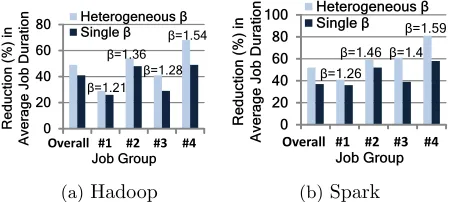
4.2 Heterogeneous Stragglers
In the previous sections, we have assumed that all jobs have the same task size distributions, i.e., have the same straggler behavior. This may not always be the case and, more generally, different classes of jobs may have different straggler behaviors. This could be specific to the jobs’ computation and input locations, or wider (but time-varying) cluster characteristics like resource contentions due to utilization and hotspots [21].
Heterogeneous straggler behaviors can have a significant impact on scheduling. In particular, if one class of jobs is likely to have stragglers more frequently, then speculation will be more valuable within those jobs. Thus, the job scheduler may want to leave more capacity for such jobs, but this extra capacity comes at the expense of other jobs, and so it is not clear how much extra capacity should be allocated.
Our analytic results highlight that the structural forms of Guidelines 1 and 2 do not change in this setting; however, the virtual sizes of the jobs are adjusted depending on the job-class βi and the specific form of the proportional sharing should be adjusted as follows. Specifically, suppose that there are two classes that have different Pareto(βi) task
size distributions. Then, our analytic results suggest that classI should be allocated
P
I Ti(t)
√ βI−1
P I
Ti(t)
√ βI−1 +
P II
Ti(t)
√ βII−1
S slots,
and the allocation among jobs within the class should then happen according to the the proportional sharing in Equation 4.1. Algorithm 4 gives the details of the design and we evaluate the gains from this generalization in §6.4. Interestingly, the form mimics the proportional sharing in Guideline 2, and the weighting of β is again by its square root. Note that the importance of (β−1) is natural since when β <2 the mean is infinite. Algorithm 4 (Heterogenous stragglers).
1. If S < β2
2
q β2−1
β1−1
P
I(t)
Ti(t), then assign all S slots to type 1 jobs.
2. If β2
2
q β2−1
β1−1
P
I(t)
Ti(t)< S ≤ β2 2
q β2−1
β1−1
P
I(t)
Ti(t)+β2 2
P
II(t)
Ti(t), then assignβ2
2
q β2−1
β1−1
P
I(t)
Ti(t)
slots to type 1 jobs and the rest to type 2 jobs.
3. IfS ≥ 2
β2
q β2−1
β1−1
P
I(t)
Ti(t) +β22 P II(t)
Ti(t), then assign
P
I(t)
Ti(t)
√ β1−1
P
I(t)
Ti(t)
√
β1−1 +
P
II(t)
Ti(t)
√ β2−1
S slots to type
1 jobs and the rest to type 2 jobs.
Given this allocation of capacity to type 1 and 2 jobs, use Algorithm ??to assign capacity
within each type.
Theorem 3. Algorithm 4 is throughput maximal.
Proof. Note, if we know the optimal scheduling algorithm assigns S1 slots to type 1 jobs andS2 slots to type 2 jobs, then we know how to allocate slots across jobs within the same type as indicated in Algorithm ??. The remaining question is how to allocate slots across different types.
Similar to proof for Theorem 1, we divide the problem into three cases. Case 1: S≤ 2
β1
P
I(t)
Ti(t)
Note that β1 < β2 gives β 2 1 4(β1−1) >
β2 2
4(β2−1), as f(x) =
x2
x−1 is a decreasing function for
x∈(1,2). When S ≤ 2
β1
P
I(t)
Ti(t), from (3.7), we know, we should assign all slots to type
1 jobs. Case 2: β2
1
P
I(t)
Ti(t)≤S ≤ β2 1
P
I(t)
Ti(t) +β2 2
P
II(t)
Ti(t) When β2
1
P
I(t)
Ti(t)≤S≤ β2 1
P
I(t)
Ti(t)+β2 2
P
II(t)
Ti(t), denote the number of slots we assign to type 1 jobs by S1 and the number of slots we assign to type 2 jobs byS2. From (3.7), unless type 1 jobs get optimal speculation level slots, no slot should be assigned to type 2 jobs. Thus, the slots assigned to type 1 and type 2 jobs should satisfy S1 ≥ β21 P
I(t)
and S2≤ β22 P
II(t)
Ti(t). The total throughput is,
β1
β1−1
X
I(t)
Ti(t)− 1 (β1−1)S1
(X
I(t)
Ti(t))2+ β 2 2 4(β2−1)
S2
= β1
β1−1
X
I(t)
Ti(t)− 1 (β1−1)S1
(X
I(t)
Ti(t))2+ β 2 2 4(β2−1)
(S−S1)
= β1
β1−1
X
I(t)
Ti(t) + β 2 2 4(β2−1)
S− 1
(β1−1) (X
I(t)
Ti(t))2 1
S1
− β
2 2 4(β2−1)
S1 (4.2)
≤ β1
β1−1
X
I(t)
Ti(t) + β 2 2 4(β2−1)
S−p β2
(β1−1)(β2−1)
X
I(t)
Ti(t),
where the last line follows from a2+b2 ≥2ab. Equality is achieved when β22
4(β2−1)S1 = 1 (β1−1)S1(
P
I(t)
Ti(t))2, i.e.,S1= β22
q β2−1
β1−1
P
I(t)
Ti(t). And (4.2) increases forS1≤ β22
q β2−1
β1−1
P
I(t)
Ti(t) and decreases afterwards. Also note that, if S1= β22
q β2−1
β1−1
P
I(t)
Ti(t), thenS1 ≥ β21 P
I(t)
Ti(t). Thus, whenβ21 P I(t)
Ti(t)≤S≤ β21 P I(t)
Ti(t)+
2
β2
P
II(t)
Ti(t), the optimal scheduling should:
1. whenS < β2
2
q β2−1
β1−1
P
I(t)
Ti(t), assign allS slots to type 1 jobs.
2. when β2 2
q β2−1
β1−1
P
I(t)
Ti(t) < S ≤ β21 P
I(t)
Ti(t) + β22 P
II(t)
Ti(t), assign β22 q
β2−1
β1−1
P
I(t)
Ti(t)
slots to type 1 jobs and the rest to type 2 jobs.
Case 3: S≥ β2 1
P
I(t)
Ti(t) +β2 2
P
II(t)
Ti(t) When S ≥ β2
1
P
I(t)
Ti(t) + β2 2
P
II(t)
Ti(t), similarly, from (3.7), in optimal scheduling, the number of slots assigned to type 1 jobs should be no less than the optimal speculation scheduling level, so S1 ≥ β21 P
I(t)
1. If S2 ≤ β22 P
II(t)
Ti(t), which implies S −S1 ≤ β22 P
II(t)
Ti(t), as we already proved,
S1= max{β22
q β2−1
β1−1
P
I(t)
Ti(t), S−β2 2
P
II(t)
Ti(t)}, and S2=S−S1. Specifically,
(a) when β2 2
q β2−1
β1−1
P
I(t)
Ti(t) ≥ S − β2 2
P
II(t)
Ti(t), if S1 ≥ β21 P
I(t)
Ti(t) and S2 ≤ 2
β2
P
II(t)
Ti(t) in optimal scheduling, thenS1 = β22
q β2−1
β1−1
P
I(t)
Ti(t) andS2 =S−S1.
(b) when β2 2
q β2−1
β1−1
P
I(t)
Ti(t) < S − β2 2
P
II(t)
Ti(t), if S1 ≥ β21 P
I(t)
Ti(t) and S2 ≤ 2
β2
P
II(t)
Ti(t) in optimal scheduling , thenS1 =S−β22 P
II(t)
Ti(t) andS2 =S−S1.
2. IfS2 ≥ β22 P
II(t)
Ti(t), which impliesS−S1 ≥ β22 P
II(t)
Ti(t), total throughput is,
β1
β1−1
X
I(t)
Ti(t)− 1 (β1−1)S1
(X
I(t)
Ti(t))2+ β2
β2−1
X
II(t)
Ti(t)− 1 (β2−1)S2
(X
II(t)
Ti(t))2
= β1
β1−1
X
I(t)
Ti(t) + β2
β2−1
X
II(t)
Ti(t)−
1 (β1−1)S1
(X
I(t)
Ti(t))2−
1 (β2−1)S2
(X
II(t)
Ti(t))2
≤ β1
β1−1
X
I(t)
Ti(t) + β2
β2−1
X
II(t)
Ti(t)−
1
S1+S2
r
1
β1−1
X
I(t)
Ti(t) + r
1
β2−1
X
II(t)
Ti(t)
2
= β1
β1−1
X
I(t)
Ti(t) + β2
β2−1
X
II(t)
Ti(t)− 1
S
r
1
β1−1
X
I(t)
Ti(t) +
r
1
β2−1
X
II(t)
Ti(t)
2
,
(4.3)
where the inequality follows from Cauchy-Schwartz inequality.
Equality is achieved whenS1 =
P
I(t)
Ti(t)
√ β1−1
P
I(t)
Ti(t)
√
β1−1 +
P
II(t)
Ti(t)
√ β2−1
S
Combining above two results, when β2 2
q β2−1
β1−1
P
I(t)
Ti(t) < S− β2 2
P
II(t)
the optimal assignment from case 2 is the global optimal assignment. But, when 2
β2
q β2−1
β1−1
P
I(t)
Ti(t)≥S−β22 P II(t)
Ti(t), it still remain unclear which assignment is
op-timal. Thus, in next step, we compare the maximum total throughput in two cases under that setting.
(a) In case 1, from (4.2), throughputµs= β1
β1−1
P
I(t)
Ti(t)+ β22 4(β2−1)S−
β2 √
(β1−1)(β2−1)
P
I(t)
Ti(t)
(b) In case 2, from (4.3), throughputµl = β1β−11
P
I(t)
Ti(t)+β2β−21
P
II(t)
Ti(t)−S1 q
1
β1−1
P
I(t)
Ti(t) + q
1
β2−1
P
II(t)
Ti(t)
!2
µs−µl= β1
β1−1
X
I(t)
Ti(t) + β22
4(β2−1)
S−p β2
(β1−1)(β2−1)
X
I(t)
Ti(t)
−
β1
β1−1
X
I(t)
Ti(t) + β2
β2−1
X
II(t)
Ti(t)−
1 S r 1
β1−1
X
I(t)
Ti(t) + r
1
β2−1
X
II(t)
Ti(t) 2 = β 2 2 4(β2−1)
S+ 1
S
r
1
β1−1
X
I(t)
Ti(t) + r
1
β2−1
X
II(t)
Ti(t)
2
−p β2
(β1−1)(β2−1)
X
I(t)
Ti(t)− β2
β2−1
X
II(t)
Ti(t)
≥√ β2
β2−1
r
1
β1−1
X
I(t)
Ti(t) +
r
1
β2−1
X
II(t)
Ti(t)
−p β2
(β1−1)(β2−1)
X
I(t)
Ti(t)− β2
β2−1
X
II(t)
Ti(t)
=0
The above result implies when β2 2
q β2−1
β1−1
P
I(t)
Ti(t) ≥ S − β22 P II(t)
Ti(t), the optimal
assignment from case 1 is the global optimal assignment. In summary, the optimal scheduling should:
1. IfS < β2
2
q β2−1
β1−1
P
I(t)
2. Ifβ2 2
q β2−1
β1−1
P
I(t)
Ti(t)< S ≤ β22 q
β2−1
β1−1
P
I(t)
Ti(t)+β22 P II(t)
Ti(t), then assign β22 q
β2−1
β1−1
P
I(t)
Ti(t)
slots to type 1 jobs and the rest to type 2 jobs.
3. IfS ≥ β2 2
q β2−1
β1−1
P
I(t)
Ti(t) +β2 2
P
II(t)
Ti(t), then assign
P
I(t)
Ti(t)
√ β1−1
P
I(t)
Ti(t)
√
β1−1 +
P
II(t)
Ti(t)
√ β2−1
S slots to type
Chapter 5
Hopper
: Design and Implementation
In this section, we build our system,Hopper, based on the theoretical guidelines. Hopperis implemented inside Hadoop [15] and Spark [3] compute frameworks.
5.1 Data Locality
Implicit in our model’s goal of allocating slots to jobs is the assumption that all the slots are equivalent. In practice, however, tasks have preferences towards machines with specific characteristics [22]. The dominant instance of such preferences isdata locality, i.e., execute tasks on the same machine as their input. With the trend towards in-memory storage [3, 23], reading data from local memory is appreciably faster than remote reads over the network. As these tasks are predominantly IO-intensive, data locality is crucial.
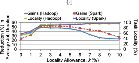
As per our guidelines, however, tasks of the next best job to schedule may not have memory local slots available [21]. Our analysis shows that memory locality drops from 98% of tasks with currently deployed techniques to as low as 54% if scheduled purely based on our guidelines without regard to memory locality. Not only are the tasks not achieving memory locality slowed down, the ensuing increase in network traffic also slows down the data transfers of intermediate phases.
memory locality on the available slots. Among these smallest k% jobs, we pick the one which can achieve memory locality for the maximum number of tasks. Further, once we pick a job, we schedule all its tasks (so that a few unscheduled tasks do not delay it) before resuming to the scheduling order as per our guidelines. In practice, a small value of k
suffices (≤5%) due to high churn in task completions and slot availabilities (evaluated in
§6.4.1).
5.2 Estimating Intermediate Data Sizes
Recall from §4.1 that our scheduling guidelines recommend scaling every job’s allocation by√αin the case of DAGs. The factorαis the ratio of the amounts of work remaining in the downstream phase over the amounts of works remaining in the upstream phase of the job’s DAG. The purpose of the scaling is to ensure pipelining of the reading of upstream tasks’ outputs over the network.
The key to calculating α is estimating the size of the intermediate output produced by tasks. Unlike the job’s input size, intermediate data sizes are not known upfront. We predict intermediate data sizes based on similar jobs in the past. Clusters typically have many recurring jobs that execute periodically as newer data streams in, and produce intermediate data of similar sizes.
For multi-waved jobs [23, 24],Hoppercan do better. It uses the ratio of intermediate to input data of the completed tasks as a predictor the future (incomplete) tasks. Data from Facebook’s and Microsoft Bing’s clusters (described in§6.1) shows that while the ratio of input to output data size of tasks vary from 0.05 all the way to 18, the ratioswithintasks of a phase have a coefficient-of-variation of only 0.07 and 0.24 at median and 90th percentile, thus lending themselves to effective learning. Hoppercalculates α as the ratio of the data remaining to be read (by downstream tasks) over the data remaining to be produced (by upstream tasks).
downstream phase reading the output from the running phase. Further, the usage of α
is generically applicable to all communication patterns of intermediate data (e.g., many-to-one, all-to-all) as it only considers the amount of data outputted and read (shown in
§6.2.1)
5.3 System Implementation
We implement Hopper inside two frameworks: Hadoop YARN (version 2.3) and Spark (version 0.7.3). Hadoop jobs read data from HDFS [25] while Spark jobs read from in-memory RDDs. Consequently, Spark tasks finish faster than Hadoop tasks for the same input size.
Briefly, these frameworks implement two level scheduling where a centralresource man-ager assigns slots to the different job managers. When a job is submitted to the resource manager, a job manager is started on one of the machines, that then executes the job’s DAG of tasks. The job manager negotiates with the resource manager for resources for its tasks.
Chapter 6
Evaluation
We evaluate our prototype ofHopperon a 200 node cluster using production workloads from Facebook and Microsoft Bing. We presentHopper’s overall gains in§6.2, fairness results in
§6.3, and design implications in §6.4.
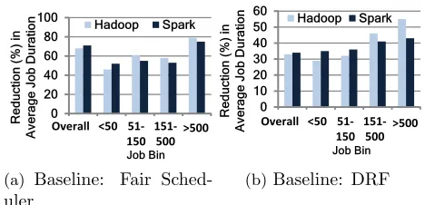
1. Hopperimproves the average job duration by 50% compared to SRPT scheduling and 70% compared to fair schedulers.
2. Hopper’s balancing of fairness and performance ensures that only 4% of jobs slow down and by≤5%.
6.1 Setup
Workload: Our evaluation is based on traces from Facebook’s production Hadoop [15] cluster (3,500 machines) and Microsoft Bing’s Dryad cluster (O(1000) machines) from Oct-Dec 2012. The traces capture over a million jobs (experimental & production). The tasks had diverse resource demands of CPU, memory and IO, varying by a factor of 24×. To create our workload, we retain the inter-arrival times of jobs, their input sizes and number of tasks, resource demands as well as job scripts.
0 20 40 60 80 100 Hadoop Spark Job Bin R e d u c ti o n ( % ) in A v e ra g e J o b D u ra ti o n
KǀĞƌĂůů фϱϬ ϱϭͲ
ϭϱϬ ϭϱϭͲ ϱϬϬ хϱϬϬ (a)Facebook 0 20 40 60 80 100 Hadoop Spark Job Bin R e d u c ti o n ( % ) in A v e ra g e J o b D u ra ti o n
KǀĞƌĂůů фϱϬ ϱϭͲ ϭϱϬ
ϭϱϭͲ ϱϬϬ
хϱϬϬ
(b)Bing
Figure 6.1: Hopper’s gains (Facebook and Bing workloads).
network with no over-subscription. Each experiment is repeated five times and we report the median.
Baseline: We contrast Hopper with state-of-the-art scheduling algorithms and straggler mitigation schemes. We use scheduling baselines of SRPT and fair scheduling. Fair schedul-ing is commonly used in clusters today, e.g., [8, 9], but is inefficient with respect to com-pletion time. In contrast, SRPT provides quite a competitive baseline for comcom-pletion time (at the expense of unfairness). We combine each of them with the LATE [13], Mantri [12] and GRASS [14] speculation algorithms.
6.2 Hopper’s Improvements
We first compareHopperwith SRPT. Unless specified, bothHopperand the baseline of SRPT executes the GRASS speculation algorithm per job, i.e. GRASS+Hoppervs. GRASS+SRPT; recent results have shown GRASS beats its competitors [14]. However, we also evaluate Hopper’s compatibility with other speculation algorithms (LATE, Mantri) in§6.2.2. In our experiments, we set the fairness allowance to be 10% and locality parameter k as 3% unless otherwise stated.
Overall Gains: Figure 6.1 plots Hopper’s gains in both Hadoop and Spark compared to SRPT. Jobs, overall, speedup by ∼ 50% in both prototypes (and workloads), which is significant given our aggressive baselines.
0 20 40 60 80 100 Hadoop Spark Re du c ti o n ( % ) in J o b D u ra ti o n ϭϬƚŚϮϱƚŚϱϬƚŚϳϱƚŚϵϬƚŚϵϵƚŚ Percentile (a) Distribution 0 10 20 30 40 50 60
2 3 4 5 6 7 8
Hadoop Spark Red u c ti o n ( %) i n A v e ra ge J ob Dur a ti o n
Length of Job’s DAG
(b) DAG
Figure 6.2: (a) Hopper’s gains at various percentiles, and (b) gains as the length of the job’s DAG varies.
the small jobs. Nonetheless,Hopper’s smart allocation of speculative slots offers 29%−40% improvement. Gains for large jobs, in contrast, are over 80%. This not only shows that there is sufficient room for the large jobs despite favoring small jobs (due to the power law in distribution of job sizes [23, 11]) but also that the value of deciding between speculative tasks and unscheduled tasks of other jobs increases with the number of tasks in the job. With trends of smaller tasks and hence, larger number of tasks per job [24], Hopper’s allocation will become important. (b) Second, gains for Spark are consistently higher (albeit, only modestly). Spark’s small task durations makes it more sensitive to stragglers and thus it spawns many more speculative copies. This makes Hopper’s scheduling more crucial.
Given the similarity in results (and for brevity), we only present the Facebook work-load’s results from now.
Distribution of Gains: Figure 6.2a plots the distribution of gains across jobs. While the median gains are just higher than the average, there is a>70% gains at higher percentiles. The encouraging aspect is that gains even at the 10th percentile are 14% and 22% in our Hadoop and Spark prototypes, respectively, which shows Hopper’s ability to improve even the worse case performance.
6.2.1 DAG of Tasks
lengths by modifying the input script of the job to contain the required number of phases, and enforce pipelining of data transfers of downstream phases with upstream tasks [26]. The communication patterns in the DAGs are varied (e.g., all-to-all, many-to-one etc.) and thus the results also serve to underscoreHopper’s generality. As Figure 6.2b shows, name’s gains continue to hold with the job’s DAG length.
Recall from §4.1 that we use a factor α for pipelined downstream communication. To appropriately capture the network-intensiveness of the downstream phase, we use a dampening value for α.1 For Spark jobs with fast in-memory map phases, intermediate data communication is the bottleneck, and a dampening value of 0.8 works best. Hadoop jobs spend most of their time in the map phase [23], and we use a dampening value of 0.3. 6.2.2 Speculation Algorithm
We now experimentally evaluateHopper’s performance with the different speculation mech-anisms that are proposed and deployed. LATE [13] is deployed in Facebook’s clusters, Mantri [12] is in operation in Microsoft Bing, and GRASS [14] is a recently reported strag-gler mitigation system that was demonstrated to perform near-optimal speculation. Our experiments in this section still use SRPT as the baseline but pair with the different strag-gler mitigation algorithms (e.g., LATE+SRPT vs. LATE+Hopper, and so forth). Figure 6.3 plots the results. We show results for Hadoop only due to space restrictions. The results for Spark are similar.
While the earlier results were achieved in conjunction with GRASS, a remarkable point is the similarity in gains even with LATE and Mantri. This indicates that as long as the straggler mitigation algorithms are aggressive in asking for speculative copies, Hopper will appropriately allocate as per the optimal speculation level. Overall, it emphasizes the aspect that resource allocation across jobs (with speculation) has a higher performance value than straggler mitigation within jobs.
1