Mode decision acceleration for H.264/AVC to SVC temporal video transcoding

(1)

R E S E A R C H

Open Access

Mode decision acceleration for H.264/AVC to SVC

temporal video transcoding

Chia-Hung Yeh

*

, Wen-Yu Tseng and Shih-Tse Wu

Abstract

This study presents a fast video transcoding architecture that overcomes the complexity of different coding structures between H.264/AVC and SVC. The proposed algorithms simplify the mode decision process in SVC owing to its heavy computations. Two scenarios namely transcoding with the same quantization parameter and bitrate reduction are considered. In the first scenario, SVC’s modes are determined by the probability models, including conditional probability, Bayesian theorem, and Markov chain. The second scenario measures MB activity to determine SVC’s modes. Experimental results indicate that our algorithm saves significant coding time with negligible PSNR loss over that when using a cascaded pixel-domain transcoder.

Keywords:Bayesian theorem, H.264/AVC, Markov, SVC, Video transcoding

Introduction

Among the many multimedia services that offer univer-sal multimedia access on heterogeneous networks in-clude videoconferencing, distance learning, and video on demand [1-4]. Such applications require a variety of devices, access links, and resources. In particular, video transcoding enables a pre-coded video to satisfy the con-straints of transmission networks or specific applications [5-15], as shown in Figure 1.

The Joint Video Team consists of ITU-T VCEG, and ISO/IEC MPEG has a standardized SVC, which is an extended version of H.264/AVC. SVC provides scalable functionality by parsing and extracting a partial bit-stream to satisfy various terminal requirements and net-work conditions. However, most conventional video contents have a non-scalable format such as H.264/ AVC. Therefore, video transcoding from non-scalable H.264/AVC to SVC is advisable for reducing computa-tions when transcoding without sacrificing R-D perform-ance. Because of codec incompatibilities between H.264/ AVC and SVC, video format transformation must de-code an original video into an intermediate format and re-encode it to SVC. While the decoding overhead is negligible, the high complexity of the encoding process still slows down the transcoding speed even when it is

on a modern multicore processor. Such a delay in speed limits its applications.

Cascaded pixel-domain transcoder (CPDT) is a

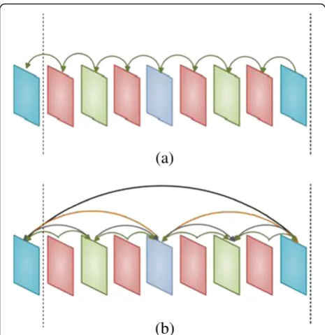
straightforward method for transcoding an existing for-mat to another [5]. The visual quality of CPDT is op-timal because the CPDT fully decoded bitstream of CPDT re-encodes it as a new one, resulting in a large computational complexity. The ability to reuse infor-mation of the incoming bitstream as much as possible can significantly reduce the computations of transcod-ing. However, H.264/AVC and SVC differ in coding structures, as illustrated in Figure 2, apparently making it impossible to directly reuse the H.264/AVC modes to those of SVCs’.

This study presents a fast algorithm for transcoding the coding format from H.264/AVC to SVC. First, H.264/AVC to SVC transcoding with the same QP is proposed. The proposed algorithm develops a mode probability model for coding format transcoding from H.264/AVC to SVC, based on the use of conditional probability, Bayesian theorem, and the Markov chain. Experimental results show that the proposed algorithm saves an average of 76.65% coding time with 0.1 dB PSNR loss over that when using a CPDT. In the second part, we discuss video transcoding from H.264/AVC to SVC with bitrate reduction. The residual DCT-domain MB energy obtained from H.264/AVC decoding process is used to find MB activity for the mode decision in SVC

* Correspondence:[email protected]

Department of Electrical Engineering, National Sun Yat-sen University, Kaohsiung 804, Taiwan

(2)

encoder [16]. The proposed algorithm saves an average of 59.4% coding time with 6.24% bitrate increase over that when using a CPDT.

The rest of this article is organized as follows.“Related study” section describes the previous aspects of video transcoding. “Proposed video transcoding from H.264/

AVC to SVC” section then introduces the proposed

video transcoding algorithm. Next, “Experimental

results” section evaluates the performance of the pro-posed method, based on the experimental results. Con-clusions are finally drawn in“Conclusions”section.

Related study

Visual quality and coding time are of priority concern during the design phase of video transcoding. Previous work can be categorized into transcoding in the fre-quency domain and transcoding in the pixel domain. De Cock et al. [17] proposed a video transcoding scheme in the frequency domain from H.264/AVC to SVC in order to reduce the coding time and complexity. Although capable of avoiding the inverse transform process to save computations, frequency transcoding degrades video quality owing to the drift problem. The study of [18] developed a scheme to transcode a single layer H.264/ AVC bitstream into SNR scalable SVC bitstreams in CGS layer. To avoid the drift problem, this study uses a re-quantization error compensation method to prevent error propagation. However, visual quality of this method has an obvious gap compared to that of CPDT.

In pixel-domain transcoding, Garrido-Cantos et al. [19] developed a method for transcoding from H.264/ AVC to SVC in temporal scalability in order to reduce computational complexity. The decoded motion vectors of H.264/AVC construct a reduced search area to accel-erate the motion estimation process in SVC. However, their scheme does not discuss the mode decision, which is computationally intensive.

Al-Muscati and Labeau [20] also developed a video transcoding approach from H.264/AVC to SVC in tem-poral scalability. Extracted from H.264/AVC bitstream, the motion vectors are used to map either the hierarch-ical B frame or zero-delay referencing structures in SVC; in addition, H.264/AVC’s modes are directly reused. Re-using coding modes is an inefficient approach owing to different coding structures between H.264/AVC and SVC, subsequently degrading the coding performance significantly.

Device profile

Transmission profile

User profile

Bit rate adaption

Frame rate adaption

Frame size adaption Standard conversion

Video source

Transcoder

Output video

Control module

Decoder Encoder

Figure 1Architecture of video transcoding.

(b)

(a)

(3)

To avoid drift problem and achieve the optimal rate distortion (RD) performance, the proposed video trans-coding scheme is in the pixel domain to eliminate drift problem and emphasize the mode decision process. Therefore, the proposed architecture has a low computa-tional complexity and satisfactory coding performance in terms of video transcoding.

Proposed video transcoding from H.264/AVC to SVC

This section introduces the proposed H.264/AVC to SVC video transcoder scheme, capable of maintaining the visual quality of transcoded videos and reducing the coding time of transcoding simultaneously.

Transcoding with the same QP

Some candidate modes are selected from those of H.264/AVC incoming bitstream by using conditional probability. The conditional probability is statistical mode distribution, consisting of the SVC’s mode distri-bution for a given mode distridistri-bution of H.264/AVC. Next, whether the current mode is the best one is deter-mined based on Bayesian theorem. Finally, Markov chain uses transitional probability to predict the likelihood of another candidate mode. The training sets of conditional probability, Bayesian theorem detection, and Markov chain consist of Football, Flower, Foreman, Carphone, and Mobile with CIF format and each sequence contain 200 frames. The quantization parameter is set to 25 and 35 while considering both low and high bitrates.

Candidate mode selection through conditional probability

Reducing computational complexity depends on the ability to efficiently reuse the information of the incom-ing bitstream. Despite the inability to apply the modes of

H.264/AVC to SVC directly, the H.264/AVC’s modes

provide hints on how to predict SVCs’. Therefore, based on an analysis of the mode distribution of these two standards, this study develops a conditional probability model to select candidate modes. Some useful candidate modes are determined by the highest conditional

probability of the SVC’s mode given the H.264/AVC’s mode. Here, Mode0 to Mode6 represent Skip mode, Inter16 × 16, Inter16 × 8, Inter8 × 16, Inter8 × 8, Intra16 × 16, and Intra4 × 4. Table 1 summarizes the statistical results of the mode distribution between H.264/AVC and SVC.

Analysis results verify the mode relations between H.264/AVC and SVC. Also, the mode extracted from the input bitstream is regarded as the candidate mode of SVC. Moreover, a linear map is found between the modes of H.264/AVC and SVC. The map can be repre-sented as Equation (1).

f :ModeH:264=AVC !ModeSVC: ð1Þ Next, the current mode in SVC is determined based on the highest conditional probability. The mode can be shown mathematically as follows.

V ¼ModeH:264=AVC_T ¼½v0v1. . .v6

ð2Þ

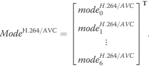
In Equation (2), T denotes a 7 × 7 transition matrix which consists of statistical results of mode distribution in H.264/AVC and SVC. ModeH:264=AVC _{can be} repre-sented as

ModeH:264=AVC ¼

modeH0:264=AVC

modeH1:264=AVC

⋮

modeH6:264=AVC

2 6 6 6 6 6 4

3 7 7 7 7 7 5 T

: ð3Þ

In Equation (3), if the mode is not utilized in the current MB of H.264/AVC, modeiH.264/AVC is defined as 0; in contrary, modeiH.264/AVC is defined as 1, where i2{1,2,. . .,6}. Finally, the maximum conditional prob-ability is obtained to determine the candidate mode of SVC.

X¼ arg max

i2f0;1;...;6gvi: ð4Þ

Table 2 defines the correlation between X and ModeSVC in Equation (4). Equations (1)–(4) are used

Table 1 Conditional probability of the SVC’s mode distribution

The mode distribution in SVC

Mode0 Mode1 Mode2 Mode3 Mode4 Mode5 Mode6

The mode distribution Mode0 0.7105 0.1862 0.0304 0.0277 0.0146 0.0083 0.0223

in H.264/AVC Mode1 0.3363 0.3520 0.0969 0.0804 0.0839 0.0016 0.0490

Mode2 0.2325 0.2776 0.2232 0.0684 0.1405 0.0007 0.0570

Mode3 0.2458 0.2731 0.0802 0.1894 0.1349 0.0007 0.0759

Mode4 0.2192 0.2120 0.1321 0.1102 0.2770 0.0000 0.0495

Mode5 0.3951 0.2428 0.1194 0.0597 0.0163 0.0313 0.1355

(4)

to obtain the highest probability of the SVC’s mode given the H.264/AVC’s mode to be the SVC’s candi-date mode.

Mode testing by Bayesian theorem detection

Among the neighboring MBs that correlate with each other in terms of motion vector, RD value, and mode, many works inherited this property and developed algorithms. As a simple formula, Bayesian theorem cal-culates conditional probability and can be used to compute posterior probabilities given some observa-tions. Here, the mode status of the neighboring MBs (top and left) is observed with respect to the current MB. The mode of the current MB selected by condi-tional probability model is assumed here to be highly correlated with its neighboring MBs’. Therefore, a Bayesian theorem detection scheme is constructed by using the spatial correlation property. Accuracy of the candidate mode is then tested by using the Bayesian theorem detection scheme. Table 3 shows the

probabil-ity distribution of the current MB’s mode in SVC.

Tables 4 and 5 show the conditional probability of the current MB’s mode given the top MB’s mode and left MB’s mode, respectively. Whether an error prediction occurs in the current MB is determined based on the Bayesian theorem detection scheme, as shown in Equa-tion (5), which applies the condiEqua-tional probability and posterior probability.

P Xð ¼xjY ¼yÞ ¼P Yð ¼yjX ¼xÞ P Xð ¼xÞ P Yð ¼yÞ ; ð5Þ

where X denotes the top (or left) MB mode and Y

represents the current MB mode. Also, X and Y 2

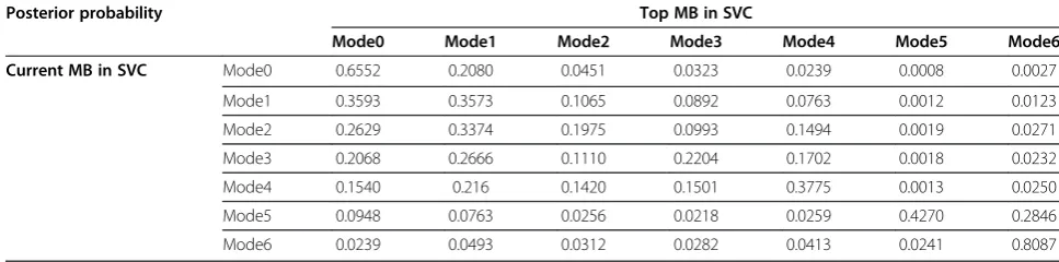
{Mode0–6}. Tables 6 and 7 show the posterior prob-ability of the top MB’s mode given the current MB’s mode. A situation in which the candidate mode in SVC lacks the highest posterior probability, suggests that the candidate mode is probably not the optimal one. Next, the mode must be predicted by using the Markov chain.

Mode refinement by Markov chain

Markov chain is used to obtain the mode when the Bayesian theorem determines that the candidate mode may be incapable of encoding efficiently. As a discrete time process, Markov chain predicts a future state by past and present states. Past, present, and future states are independent of each other because Markov chain has the feature of stationary transition. Based on the fea-ture of Markov chain, fufea-ture states can be predicted by the current state. Markov chain can be represented by

P S nþ1¼snjS1¼s1;S2¼s2;. . .;Sn¼sn

¼P S nþ1¼snþ1jSn_¼_sn_; _ð6Þ

where a finite set of states as

S2fs0;s1;. . .;sk1g; ð7Þ

where k denotes the number of states. The Markov

property states that the conditional probability distribu-tion predicts the future state since its state depends only on the past and the current state of the system. The changes of state are called transitions, and the probabil-ities associated with various state-changes are called transition probabilities. The transition probability can be shown as

ti;j¼P Snþ1¼sjjSn¼si

; ð8Þ

where the index i, j2 {0, 1, . . ., k – 1}. The set of all states and transition probabilities characterizes com-pletely a Markov chain. These transition probabilities can be shown as a transition probability matrix. Notably, the sum of each row of transition matrix is equal to 1. It can be shown as

Xk1

j¼0

ti;j¼1: ð9Þ

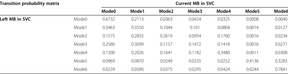
Here, the mode in SVC can be regarded as a state in the Markov chain. Transition matrix consists of both vertical and horizontal correlations. Vertical transitional probability is the mode distribution of the current MB given the top MB’s mode distribution. Horizontal transi-tional probability is the mode distribution of the current MB given the left MB’s mode distribution. Tables 8 and 9 show the vertical transition and horizontal transition matrices, respectively.

A situation in which the candidate mode cannot pass Bayesian theorem suggests that this mode selected by conditional probability may be incapable of coding. Table 2 The correlation between X and ModeSVC

ModeSVC mode0

SVC

mode1 SVC

mode2 SVC

mode3 SVC

mode4 SVC

mode5 SVC

mode6 SVC

X 0 1 2 3 4 5 6

Table 3 Mode distribution in SVC

(5)

Table 4 Conditional probability of the current MB’s mode

Conditional probability Current MB in SVC

Top MB in SVC Mode0 0.6552 0.2139 0.0541 0.0381 0.0341 0.0010 0.0036

Mode1 0.3494 0.3573 0.1167 0.0825 0.0804 0.0014 0.0123

Mode2 0.2188 0.3078 0.1975 0.0993 0.1527 0.0013 0.0226

Mode3 0.1756 0.2883 0.1111 0.2204 0.1805 0.0013 0.0228

Mode4 0.1079 0.2051 0.1389 0.1415 0.3775 0.0012 0.0278

Mode5 0.0769 0.0653 0.0358 0.0313 0.0268 0.4270 0.3370

Mode6 0.0184 0.0492 0.0375 0.0287 0.0372 0.0204 0.8087

Table 5 Conditional probability of the current MB’s mode

Conditional probability Current MB in SVC

Left MB in SVC Mode0 0.6729 0.2112 0.0363 0.0424 0.0325 0.0008 0.0040

Mode1 0.3459 0.3546 0.1043 0.1009 0.0803 0.0014 0.0127

Mode2 0.1576 0.2835 0.2622 0.0955 0.1762 0.0016 0.0234

Mode3 0.2577 0.3095 0.1155 0.1470 0.1416 0.0016 0.0271

Mode4 0.1306 0.2036 0.1650 0.1188 0.3498 0.0011 0.0310

Mode5 0.0969 0.0871 0.0250 0.0235 0.0252 0.4138 0.3285

Mode6 0.0239 0.058 0.0375 0.0295 0.0424 0.0244 0.7843

Table 6 Posterior probability of the top MB’s mode

Posterior probability Top MB in SVC

Current MB in SVC Mode0 0.6552 0.2080 0.0451 0.0323 0.0239 0.0008 0.0027

Mode1 0.3593 0.3573 0.1065 0.0892 0.0763 0.0012 0.0123

Mode2 0.2629 0.3374 0.1975 0.0993 0.1494 0.0019 0.0271

Mode3 0.2068 0.2666 0.1110 0.2204 0.1702 0.0018 0.0232

Mode4 0.1540 0.216 0.1420 0.1501 0.3775 0.0013 0.0250

Mode5 0.0948 0.0763 0.0256 0.0218 0.0259 0.4270 0.2846

Mode6 0.0239 0.0493 0.0312 0.0282 0.0413 0.0241 0.8087

Table 7 Posterior probability of the left MB’s mode

Posterior probability Left MB in SVC

Current MB in SVC Mode0 0.6729 0.2087 0.0352 0.0475 0.0305 0.001 0.0036

Mode1 0.3500 0.3546 0.1049 0.0945 0.0788 0.0015 0.0145

Mode2 0.1626 0.2818 0.2622 0.0953 0.1726 0.0012 0.0253

Mode3 0.2298 0.3303 0.1156 0.1470 0.1506 0.0013 0.0241

Mode4 0.1392 0.2074 0.1685 0.1118 0.3498 0.0011 0.0274

Mode5 0.0737 0.0778 0.0348 0.0279 0.0247 0.4138 0.3479

(6)

Another mode for improving coding performance is pre-dicted using the Markov chain. The mode of the current MB is predicted from the left (or top) side MB by transi-tion matrix. It can be represented as (10)

f :Modet1;SVC!Modet;SVC; ð10Þ

where t – 1 and t denote the neighboring MB and

current MB, respectively. The transition probability can be illustrated as follows.

t_i;j¼P Sn¼snSn1¼sn1

ð11Þ

where the indexi, j2{1, 2, . . ., 7}. Markov chain uses a certain state to predict the future state. This study attempts to accurately predict the current MB’s mode by using the Markov chain. This mode is illustrated in Equation (12).

V¼Modet1;SVCT

¼

modet01;SVC

modet11;SVC

⋮

modet61;SVC

2 6 6 6 6 4

3 7 7 7 7 5

T

t00 t01 . . . t06

t10 t11 . . . t16

⋮ ⋮ . . . ⋮

t60 t61 . . . t66

2 6 6 4

3 7 7 5

¼½v0v1. . .v6

ð12Þ

whereT denotes a transition matrix which is the statis-tical results of mode distribution between the current

MB and the left (or top) side of the current MB in SVC. Also,tijdenotes the element which is transitional

probabil-ity ofT. In Equation (12), if the mode is not utilized in the left (or top) side of the current MB in SVC, modeiH.264/AVCis

defined as 0. In contrast, if the mode is utilized in the left (or top) side of the current MB in SVC, modeiH.264/AVCis

defined as 1, wherei2{1, 2,. . ., 6}. The highest value is then obtained. This value can be shown as follow

X¼ arg max

i2f0;1;...;6gvi: ð13Þ

Table 10 defines the correlation ofX and Modet,SVC. In conclusion, the candidate mode is first selected by the con-ditional probability model. Next, whether this candidate model is satisfactory is verified by using Bayesian theorem. If not, another mode for coding is predicted by using Mar-kov chain. The proposed algorithm can avoid an exhaust-ive mode search without sacrificing the RD performance.

Transcoding with bitrate reduction

Table 11 shows the statistic results of the mode distribu-tion between H.264/AVC and SVC when transcoded from high to low bitrates. We observe that Mode0 and Mode1 have high probability to be chosen in SVC. In bitrate reduction transcoding, SVC encoder usually selects large block size such as Mode0 and Mode1 to be the optimal mode and large QP to make the residual smaller to meet the transcoding requirement.

Table 8 Vertical transition probability matrixes

Transition probability matrix Current MB in SVC

Top MB in SVC Mode0 0.6768 0.2209 0.0559 0.0393 0.0352 0.0010 0.0037

Mode1 0.3487 0.3565 0.1165 0.0823 0.0802 0.0014 0.0123

Mode2 0.2035 0.2862 0.1836 0.0923 0.1420 0.0012 0.0210

Mode3 0.1756 0.2882 0.1111 0.2204 0.1805 0.0013 0.0228

Mode4 0.1012 0.1924 0.1303 0.1328 0.3542 0.0012 0.0261

Mode5 0.0804 0.0683 0.0374 0.0327 0.0281 0.4467 0.3526

Mode6 0.0183 0.0489 0.0372 0.0285 0.0370 0.0202 0.8033

Table 9 Horizontal transition probability matrixes

Transition probability matrix Current MB in SVC

Left MB in SVC Mode0 0.6732 0.2113 0.0363 0.0424 0.0325 0.0008 0.0040

Mode1 0.3463 0.3550 0.1044 0.101 0.0804 0.0014 0.0127

Mode2 0.1575 0.2832 0.2619 0.0954 0.1760 0.0016 0.0234

Mode3 0.2580 0.3099 0.1157 0.1472 0.1418 0.0016 0.0271

Mode4 0.1300 0.2026 0.1641 0.1182 0.3480 0.0011 0.0308

Mode5 0.0969 0.0870 0.0249 0.0235 0.0252 0.4136 0.3283

(7)

According to MB activity, each MB in H.264/AVC can be classified into a complexity or homogenous region [16]. The MB’s mode in SVC can be predicted through the information of MB activity obtained from H.264/ AVC decoding process. We joint consider the relation between MB activity and mode distribution between H.264/AVC and SVC to decide the modes in SVC to avoid exhaustively searching all modes in transcoding process.

To obtain MB activity, the average energy of MB should be calculated first. The MB energy (EMB) is defined as the absolute DCT coefficient values summa-tion of MB, as shown in Equasumma-tion (14).

EMB¼ 1 256

X15

α¼0

X15

β¼0

coeff½ α½ β

j j; ð14Þ

where coeff represents the DCT coefficient within each 4 × 4 sub-block.αis the number of 4 × 4 sub-blocks and βis the pixel position. Then, the average energy of frame is calculated for MB activity, as shown in Equation (15).

Eframe¼ 1 NM

X

N1

u¼0

X

M1

v¼0 coeff u ½ ½ v

j j; ð15Þ

whereNandMare frame size in the horizontal and ver-tical directions. u and vrepresent the position of DCT coefficient in the horizontal and vertical directions. Therefore, we use Equations (14) and (15) to build MB activity, as shown in Equation (16).

MBActivity¼ 1₀ if EMB=_elseEframe≥1:

ð16Þ

After obtaining the MB activity, we summarize the proposed algorithm of H.264/AVC to SVC bitrate reduc-tion transcoding as follows. When H.264/AVC’s MB is

Mode0 or Mode1 in H.264/AVC, the Mode0 and Mode1 are selected as the candidate modes in SVC. If MB activ-ity is equal to 0 and H.264/AVC’s MB is Mode2, Mode3, or Mode4, it means that the current MB belongs to homogeneous region.

Therefore, Mode0 and Mode1 are determined to be candidate modes. On the other hand, if MB activity is equal to 1, it means the current MB is complexity re-gion. Hence, Mode2, Mode3, and Mode4 should be added as the candidate modes in SVC. When MB

activ-ity is equal to 1 and H.264/AVC’s MB is Mode5 or

Mode6, the Mode0, Mode1, and Mode5 are chosen as the candidate modes. If MB activity is large, small block size, Mode6, is selected as the candidate modes.

Experimental results

The proposed algorithm is implemented on JM 13.2 and JSVM 9.12. Each test benchmark contains 200 frames, with one I frame followed by 199 B or P frames. The group of picture is set to 16. The maximum search range is ±16 pixels and the number of reference frame is set to 1. Two different QPs, 25 and 35, are used in the experi-ments. The proposed method is compared with two methods, i.e., fully decode and fully encode (FDFE) and mode reusing (MR).

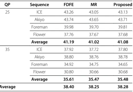
Tables 12, 13, and 14 show the comparisons of PSNR, bitrate, and coding time, respectively, with the same QP transcoding. Tables 15, 16, and 17 show the comparisons of PSNR, bitrate, and coding time, respectively, with bitrate reduction transcoding. According to these tables, the proposed algorithm significantly reduces transcoding computations with negligible PSNR loss and bitrate in-crease when compared to FDFE. According to Table 12, compared to FDFE, PSNR of the proposed algorithm only has 0.1 dB degradation. However, in this case, the proposed algorithm saves up to 76.65% coding time. In

Table 11 Statistics of mode distribution

The mode distribution in SVC with QP 25

The mode distribution Mode0 0.9373 0.0390 0.0043 0.0059 0.0006 0.0097 0.0032

in H.264/AVC with QP 15 Mode1 0.5585 0.2821 0.0560 0.0421 0.0335 0.0033 0.0245

Mode2 0.4851 0.2694 0.1184 0.0414 0.0422 0.0041 0.0394

Mode3 0.5102 0.2685 0.0486 0.0854 0.0326 0.0050 0.0497

Mode4 0.4162 0.2899 0.0966 0.0770 0.0830 0.0021 0.0351

Mode5 0.8452 0.0806 0.0118 0.0089 0.0006 0.0455 0.0075

Mode6 0.3328 0.2338 0.1029 0.0847 0.0343 0.0168 0.1947

Table 10 The correlation betweenXand Modet,SVC Modet,SVC mode0

t,SVC

mode1

t,SVC

mode2

t,SVC

mode3

t,SVC

mode4

t,SVC

mode5

t,SVC

mode6

t,SVC

(8)

Table 14 Coding time (s) comparisons of CIF format benchmarks with the same QP transcoding

QP Sequence FDFE MR Proposed

Time Time ΔTS (%) Time ΔTS (%)

25 ICE 1201.07 193.44 83.89 306.96 74.44

Akiyo 1274.57 147.35 88.44 187.92 85.26

Foreman 1342.63 318.48 76.28 486.84 63.74

Flower 1408.05 305.14 78.33 509.86 63.79

Average 1306.58 241.10 81.74 372.90 71.81

35 ICE 1183.33 149.29 87.38 203.16 82.83

Akiyo 1197.33 118.10 90.14 128.65 89.26

Foreman 1244.98 175.16 85.93 230.88 81.46

Flower 1348.59 255.53 81.05 372.60 72.37

Average 1243.56 174.52 86.13 233.82 81.48

Average 1275.07 207.81 83.94 303.36 76.65

Table 15 PSNR(dB) Comparisons of CIF format benchmarks with bitrate reduction transcoding

25 ICE 43.26 43.05 43.13

Akiyo 43.74 43.65 43.71

Foreman 39.98 39.70 39.81

Flower 37.76 37.67 37.68

Average 41.19 41.02 41.08

35 ICE 37.92 37.72 37.80

Akiyo 38.80 38.76 38.78

Foreman 34.92 34.75 34.65

Flower 30.80 30.66 30.68

Average 35.61 35.47 35.48

Average 38.40 38.25 38.28

Table 16 Bitrate (kbps) comparisons of CIF format benchmarks with bitrate reduction transcoding

25 ICE 380.07 473.37 389.42

Akiyo 143.15 183.61 143.40

Foreman 729.87 939.10 810.19

Flower 2013.45 2171.48 2075.19

Average 816.64 941.89 854.55

35 ICE 143.71 145.42 220.18

Akiyo 37.29 77.24 37.31

Foreman 220.00 386.46 239.99

Flower 540.32 658.67 555.08

Average 235.33 316.95 263.14

Average 525.99 629.42 558.85

Table 17 Coding time (s) comparisons of CIF format benchmarks with bitrate reduction transcoding

Time Time ΔTS(%) Time ΔTS(%)

25 ICE 1250.15 326.99 73.84 505.95 59.53

Akiyo 1296.49 262.72 79.74 433.76 66.54

Foreman 1362.05 556.81 59.12 565.85 58.46

Flower 1402.95 490.77 65.02 655.12 53.30

Average 1327.91 409.32 69.43 540.17 59.46

35 ICE 1180.91 326.38 72.36 493.10 58.24

Akiyo 1255.26 254.89 79.69 414.69 66.96

Foreman 1296.39 549.55 57.61 532.60 58.92

Flower 1357.46 482.59 64.45 635.51 53.18

Average 1272.51 403.35 68.53 518.98 59.33

Average 1300.21 406.34 68.98 529.58 59.40

Table 12 PSNR(dB) comparisons of CIF format benchmarks with the same QP transcoding

25 ICE 40.97 41.00 41.12

Akiyo 41.25 41.10 41.18

Foreman 38.09 37.80 37.98

Flower 36.29 36.11 36.22

Average 39.15 39.00 39.13

35 ICE 34.46 34.08 34.19

Akiyo 34.75 34.59 34.67

Foreman 32.06 31.57 31.81

Flower 27.92 27.67 27.83

Average 32.30 31.98 32.13

Average 35.73 35.49 35.63

Table 13 Bitrate (kbps) comparisons of CIF format benchmarks with the same QP transcoding

25 ICE 389.32 484.94 429.18

Akiyo 143.91 170.77 148.25

Foreman 728.65 916.84 781.67

Flower 2173.80 2364.97 2251.81

Average 858.92 984.38 902.73

35 ICE 137.25 193.43 159.52

Akiyo 34.36 45.12 34.41

Foreman 204.30 321.77 238.90

Flower 569.09 669.58 598.45

Average 236.25 307.48 257.82

(9)

bitrate reduction transcoding, Table 17 indicates that the proposed algorithm saves 59.4% coding time with only 6.24% bitrate increase and outperforms MR by 13.42% under the similar PSNR. Experimental results demon-strate that the proposed scheme has a satisfactory RD performance and low computational complexity for both low and high motion sequences.

Conclusions

This study presents a video transcoder from H.264/AVC to SVC with temporal scalability in order to maintain transcoding visual quality and save coding time simul-taneously. The proposed algorithm solves an important problem, mode prediction, when transcoding a single layer video into a multi-layer one under two different scenarios: transcoding with same QP and bitrate reduc-tion. In the first part, three probability models are also developed to screen, test, and refine modes of an incom-ing video when transcoded with the same QP. In the second part, MB activity is efficiently measured for mode determination in SVC for bitrate reduction trans-coding. Experimental results demonstrate that the

pro-posed algorithm significantly reduces transcoding

computations and only has negligible visual quality deg-radation. Therefore, video content that is encoded using single-layer H.264/AVC can benefit from the newly developed scalability features without too many trans-coding efforts.

Competing interests

The authors declare that they have no competing interests.

Acknowledgment

This work was supported by the National Science Council, R.O.C, under the Grant NSC 99-2628-E-110-008-MY3 and NSC101-2221-E-110-093-MY2.

Received: 15 July 2012 Accepted: 1 September 2012 Published: 24 September 2012

References

1. AM Thekalp,Digital Video Processing(Prentice Hall PTR, New Jersey, 1995) 2. MT Sun, AR Reibman,Compressed Video over Networks(Marcel Dekker, New

Work, 2001)

3. Y Wang, J Ostermann, YQ Zhang,Video Processing and Communications (Prentice Hall, New Jersey, 2002)

4. KN Ngan, CW Yap, KT Tan,Video Coding for Wireless Communications (Prentice Hall, New Jersey, 2002)

5. J Xin, CW Lin, MT Sun, Digital video transcoding. Proc IEEE93(1), 84–97 (2005)

6. SF Chang, A Vetro, Video adaptation: concepts, technologies, and open issues. Proc IEEE93(1), 148–158 (2005)

7. A Vetro, C Christopoulos, S Huifang, Video transcoding architectures and techniques: an overview. IEEE Signal Process Mag20(2), 18–29 (2003) 8. I Ahmad, X Wei, Y Sun, Y-Q Zhang, Video transcoding: an overview of

various techniques and research issues. IEEE Trans Multimed7(5), 793–804 (2005)

9. VA Nguyen, YP Tan, Efficient video transcoding from H.263 to H.264/AVC standard with enhanced rate control. EURASIP J. Appl. Signal Process 2006(83563), 1–15 (2006)

10. J Xin, A Vetro, H Sun, Y Su, Efficient MPEG-2 to H.264/AVC transcoding of intra-coded video. EURASIP J. Appl. Signal Process2007(75310), 1–12 (2007)

11. S Eminsoy, S Dogan, AM Kondoz, Transcoding-based error-resilient video adaptation for 3 G wireless networks. EURASIP J Appl Signal Process 2007(39586), 1–13 (2007)

12. CW Lin, YP Tan, A Vetro, A Kot, MT Sun, Video adaptation for

heterogeneous environments. EURASIP J Appl Signal Process2007(18578), 1–4 (2007)

13. H Li, Y Wang, CW Chen, An attention-information-based spatial adaptation framework for browsing videos via mobile devices. EURASIP J Appl Signal Process2007(25415), 1–12 (2007)

14. TH Tsai, YF Lin, HY Lin, Video transcoder in DCT-domain spatial resolution reduction using low-complexity motion vector refinement algorithm. EURASIP J Appl Signal Process2007(467290), 1–15 (2007)

15. A Corrales-Garcia, JL Martinez, F Fernandez-Escribano, JM Villalon, H Kalva, P Cuenca, Wyner-Ziv to baseline H.264 video transcoder. EURASIP J Appl Signal Process135, (2012 (2012)

16. X Liu, W Zhu, K-Y Yoo,Fast inter mode decision algorithm based on the MB activity for MPEG-2 to H.264/AVC transcoding, 2nd edn. (Proceedings of International Conference on Computational Science and Engineering, Vancouver, BC, 2009), pp. 25–30

17. J De Cock, S Notebaert, P Lambert, R Van de Walle, Architectures for fast transcoding of H.264/AVC to quality-scalable SVC streams. IEEE Trans Multimed11(7), 1209–1224 (2009)

18. J De Cock, S Notebaert, R Van de Walle,Transcoding from H.264/AVC to SVC with CGS layers, 4th edn. (Proceedings of IEEE International Conference on Image Processing, San Antonio, TX, 2007), pp. 73–76

19. R Garrido-Cantos, J De Cock, JL Martinez, S Van Leuven, P Cuenca, Motion-based temporal transcoding from H.264/AVC-to-SVC in baseline profile. IEEE Trans Consum Electron57(1), 239–246 (2011)

20. H Al-Muscati, F Labeau,Temporal transcoding of H.264/AVC video to the

scalable format(Proceedings of 2nd International Conference on Image

Processing Theory Tools and Applications, Paris, 2010), pp. 138–143

doi:10.1186/1687-6180-2012-204

Cite this article as:Yehet al.:Mode decision acceleration for H.264/AVC to SVC temporal video transcoding.EURASIP Journal on Advances in Signal Processing20122012:204.

Submit your manuscript to a

journal and beneﬁ t from:

7Convenient online submission

7Rigorous peer review

7Immediate publication on acceptance

7Open access: articles freely available online 7High visibility within the ﬁ eld

7Retaining the copyright to your article