Volume 2011, Article ID 973806,20pages doi:10.1155/2011/973806
Research Article
Evolutionary Approach to Improve Wavelet Transforms for
Image Compression in Embedded Systems
Rub´en Salvador,
1F´elix Moreno,
1Teresa Riesgo,
1and Luk´aˇs Sekanina
21Centre of Industrial Electronics, Universidad Polit´ecnica de Madrid, Jos´e Gutierrez Abascal 2,
28006 Madrid, Spain
2Faculty of Information Technology, Brno University of Technology, Bozetechova 2, 612 66 Brno, Czech Republic
Correspondence should be addressed to Rub´en Salvador,[email protected]
Received 21 July 2010; Revised 19 October 2010; Accepted 30 November 2010
Academic Editor: Yannis Kopsinis
Copyright © 2011 Rub´en Salvador et al. This is an open access article distributed under the Creative Commons Attribution License, which permits unrestricted use, distribution, and reproduction in any medium, provided the original work is properly cited.
A bioinspired, evolutionary algorithm for optimizing wavelet transforms oriented to improve image compression in embedded systems is proposed, modelled, and validated here. A simplified version of an Evolution Strategy, using fixed point arithmetic and a hardware-friendly mutation operator, has been chosen as the search algorithm. Several cutdowns on the computing requirements have been done to the original algorithm, adapting it for an FPGA implementation. The work presented in this paper describes the algorithm as well as the test strategy developed to validate it, showing several results in the effort to find a suitable set of parameters that assure the success in the evolutionary search. The results show how high-quality transforms are evolved from scratch with limited precision arithmetic and a simplified algorithm. Since the intended deployment platform is an FPGA, HW/SW partitioning issues are also considered as well as code profiling accomplished to validate the proposal, showing some preliminary results of the proposed hardware architecture.
1. Introduction
Wavelet Transform (WT) brought a new way to look into a signal, allowing for a joint time-frequency analysis of information. Initially defined and applied through the Fourier Transform and computed with the subband filtering scheme, known as Fast Wavelet Transform (FWT), the Discrete Wavelet Transform (DWT) widened its possibilities with the proposal of theLifting Scheme(LS) by Sweldens [1]. Custom construction of wavelets was made possible with this computation scheme.
Adaptation capabilities are increasingly being brought to embedded systems, and image processing is, by no means, the exception to the rule. Compression standard JPEG2000 [2] relies on wavelets for its transform stage. It is a very useful tool for (adaptive) image compression algorithms, since it provides a transform framework that can be adapted to the type of images being handled. This feature allows it to improve the performance of the transform according to each particular type of image so that improved compression (in
terms of quality versus size) can be achieved, depending on the wavelet used.
Having a system able to adapt its compression perfor-mance, according to the type of images being handled, may help in, for example, the calibration of image processing systems. Such a system would be able to self-calibrate when it is deployed in different environments (even to adapt through its operational life) and has to deal with different types of images. Certain tunings to the transform coefficients may help in increasing the quality of the transform and, consequently, the quality of the compression.
experts. Therefore, what is being proposed here is the use of bio-inspired algorithms, such as Evolutionary Algorithms (EAs), as a design/optimization tool to help find new wavelet filters adapted to specific kind of images. For this reason, it is the whole system that is being adapted. No extra computing effort is added in the transform algorithm, such as what classicaladaptive lifting techniques propose. In contrast, we are proposing newways to design completely new wavelet filters.
The choice of an FPGA as the computing device for the embedded system comes from the restrictions imposed by theembedded system itself. The suitability of FPGAs for high-performance computing systems is nowadays generally accepted due to their inherent massive parallel processing capabilities. This reasoning can be extended to embedded vision systems as shown in [3]. Alternative processing devices like Graphics Processing Units (GPUs) have a comparable degree of parallelism producing similar throughput figures depending on the application at hand, but their power demands are too high for portable/mobile devices [4–7].
Therefore, the scope of this paper is directed at a generic artificial vision (embedded) system to be deployed in an unknown environment during design time, letting the calibration phase adjust the system parameters so that it performs efficient signal (image) compression. This allows the system to efficiently deal with images coming from very diverse sources such as visual inspections of a manufacturing line, a portable biometric data compression/analysis system, a terrestrial satellite image, and. Besides, the proposed algorithm will be mapped to an FPGA device, as opposed to other proposals, where these algorithms need to run on supercomputing machines or, at least, need such a comput-ing power that makes them unfeasible for an implementation as an embeddedreal-timesystem.
The remainder of this paper is structured as follows. Sections2and3show a short introduction to WT and EAs. After an analysis of previously published works inSection 4, the proposed method is presented in Section 5. Obtained results are shown and discussed inSection 6, validating the proposed algorithm.Section 7analyses the implementation in an FPGA device, together with the proposed architecture able to host this system and the preliminary results obtained. The paper is concluded inSection 8, featuring a short discus-sion and commenting on future work to be accomplished.
2. Overview of the Wavelet Transform
The DWT is a multiresolution analysis (MRA) tool widely used in signal processing for the analysis of the frequency content of a signal at different resolutions.
It concentrates the signal energy into fewer coefficients to increase the degree of compression when the data is encoded. The energy of the input signal is redistributed into a low-resolution trend subsignal (scaling coefficients) and high-resolution subsignals (wavelet coefficients; horizontal, vertical, and diagonal subsignals for image transforms). If the wavelet chosen for the transform is suited for the type of image being analysed, most of the information of the signal will be kept in the trend subsignal, while the wavelet
sj
sj−1
dj−1
sj−2
dj−2
Split P −
−
U Split P U
+ +
Figure1: Lifting scheme.
coefficients (high-frequency details) will have a very low value. For this reason, the DWT can reduce the number of bits required to represent the input data.
For a general introduction to wavelet-based multireso-lution analysis check [8], theFast Wavelet Transform(FWT) algorithm computes the wavelet representation via asubband filteringscheme which recursively filters the input data with a pair of high-pass and low-pass digital filters, downsampling the results by a factor of two [9]. A widely known set of filters that build up the standard D9/7 wavelet (used in JPEG2000 for lossy compression) gets its name because its high-pass and low-pass filters have 9 and 7 coefficients, respectively.
The FWT algorithm was improved by theLifting Scheme (LS), introduced by Sweldens [1], which reduces the com-putational cost of the transform. It does not rely on the Fourier Transform for its definition and application and has given rise to the so-calledSecond Generation Wavelets[10]. Besides, the research effort put on the LS has simplified the construction of custom wavelets adapted to specific and different types of data.
The basic LS, shown inFigure 1, consists of three stages: “Split”, “Predict”, and “Update”, which try to exploit the correlation of the input data to obtain a more compact representation of the signal [11].
The Split stage divides the input data into two smaller subsets, sj−1 anddj−1, which usually correspond with the
even and odd samples. It is also called theLazy Wavelet. To obtain a more compact representation of the input data, thesj−1subset is used topredictthedj−1subset, called
the wavelet subset, which is based on the correlation of the original data. The difference between the prediction and the actual samples is stored, also as dj−1, overwriting its
original value. If the prediction operatorPis reasonably well designed, the difference will be very close to 0, so that the two subsetssj−1anddj−1produce a more compact representation
of the original data setsj.
In most cases, it is interesting to maintain some prop-erties of the original signal after the transform, such as the mean value. For this reason, the LS proposes a third stage that not only reuses the computations already done in the previous stages but also defines an easily invertible scheme. This is accomplished by updating the sj−1 subset
with the already computed wavelet set dj−1. The wavelet
representation ofsjis therefore given by the set of coefficients {sj−2,dj−2,dj−1}.
the wavelet representation{s−n,d−n,. . .,d−1}. Therefore, the
algorithm for the LS implementation is as follows
for j←1,ndo {sj,dj} ←Split(sj+1)
dj=dj−P(sj) sj=sj+U(dj)
end for
where j stands for the decomposition level. There exists a different notation for the transform coefficients{sj−i,dj−i};
for a 2-level image decomposition, it can be expressed as {LL,LH,HL,HH}, whereLstands for low-pass andH for high-pass coefficients, respectively.
3. Optimization Techniques Based on
Bioinspired, Evolutionary Approaches
Evolutionary Computation (EC) [12] is a subfield of Artifi-cial Intelligence (AI) that consists of a series of biologically inspired search and optimization algorithms that evolve iteratively better and better solutions. It involves techniques inspired by biological evolution mechanisms such as repro-duction, mutation, recombination, natural selection, and survival of the fittest.
An Evolution Strategy (ES) [13] is one of the fundamen-tal algorithms among Evolutionary Algorithms (EAs) that utilize a population of candidate solutions and bio-inspired operators to search for a target solution. ESs are primarily used for optimization of real-valued vectors. The algorithm operators are iteratively applied within a loop, where each run is called ageneration(g), until a termination criterion is met. Variation is accomplished by the so-calledmutation operator. For real-valued search spaces, mutation is normally performed by adding a normally (Gaussian) distributed random value to each component under variation (i.e., to each parameter encoded in the individuals). Algorithm 1 shows a pseudocode description of a typical ES.
One of the particular features of ESs is that the individual step sizes of the variation operator for each coordinate (or correlations between coordinates) is governed by self-adaptation (or by covariance matrix self-adaptation (CMA-ES) [14]). This self-adaptation of the step size σ, also known as mutation strength(i.e., standard deviation of the normal distribution), implies that σ is also included in the chromosomes, undergoing variation and selection itself (coevolving along with the solutions).
The canonical versions of the ES are denoted by (μ/ρ,λ)-ES and (μ/ρ+λ)-ES, whereμdenotes the number of parents (parent population,Pμ),ρ ≤ μthe mixing number
(i.e., the number of parents involved in the procreation of an offspring), andλ the number of offspring (offspring population, Pλ). The parents are deterministically selected
from the set of either the offspring, referred to as comma selection(μ < λ), or both the parents and offspring, referred to asplus selection. This selection is based on the ranking of the individuals’ fitness (F) choosing theμbest individuals out of the whole pool of candidates. Once selected,ρout of
(1)g←0
(2) InitializePμ(g)← {(ym,sm),m=1,. . .,μ}
(3) EvaluateP(μg)
(4)whilenot termination conditiondo
(5) for alll∈λdo
(6) R←Drawρparents fromP(μg)
(7) rl←recombine (R)
(8) (yl,sl)←mutate (rl)
(9) Fl←evaluate (yl)
(10) end for
(11) P(λg)← {(yl,sl),l=1,. . .,λ}
(12) P(μg+1)←selection (P(λg),P
(g)
μ ,μ, +,)
(13) g←g+ 1
(14)end while
Algorithm1: (μ/ρ+,λ)-ES.
theμ parents (R) are recombined to produce an offspring individual (rl) usingintermediate recombination, where the
parameters of the selected parents are averaged or randomly chosen ifdiscrete recombinationis used. Each ES individual
a := (y,s) comprises the object parameter vector y to be optimized and a set of strategy parametersswhich coevolve along with the solution (and are therefore being adapted themselves). This is a particular feature of ES called self-adaptation. For a general description of the (μ/ρ+, λ)-ES, see
[13].
4. Previous Work on Wavelets Adaptation
When the LS was proposed, new ways of constructing adaptive wavelets arose. One remarkable result is the one by Claypoole et al. [18] which used LS to adapt theprediction stage to minimize a data-based error criterion, so that this stage gets adapted to the signal structure. TheUpdatestage is not adapted, so it is still used to preserve desirable properties of the wavelet transform. Another work which is focused on making perfect reconstruction possible without any overhead cost was proposed by Piella and Heijmans [19] that makes the update filter utilize local gradient information to adapt itself to the signal. In this work, a very interesting survey of the state of the art on the topic is covered.
These brief comments on the current literature proposals show the trend in the research community which has mainly involved the adaptation of the transform to the local properties of the signal on the fly. This implies an extra computational effort to detect the singularities of the signal and, afterwards, apply the proposed transform. Besides, a lot of work has been published on adaptive thresholding techniques for data compression.
The work being reported on in this paper deals with finding a complete new set of filters adapted to a given signal type which is equivalent to changing the whole wavelet transform itself. Therefore, the general lifting framework still applies. This has the advantage of keeping the computational complexity of the transform at a minimum (as defined by the LS) not being overloaded with extra filtering features to adapt to these local changes in the signal (as the transform is being performed).
Therefore, the review of the state of the art covered in this section will focus on bio-inspired techniques for the automatic design of new wavelets (or even the optimization of existing ones). This means that the classical meaning of adaptive lifting (as mentioned above) does not apply in this work. Adaptive, within the scope of this work, refers to the adaptivity of the system as a whole. As a consequence, this system does not adapt at run time to the signal being analysed, but, in contrast, it is optimized previously to the system operation (i.e., during a calibration routine or in a postfabrication adjustment phase).
4.2. Evolutionary Design of Wavelet Filters. The work described here gets its original idea from [20] by Grasemann and Miikkulainen. In their work, the authors proposed the original idea of combining the lifting technique with EA for designing wavelets. As it is drawn from [1,10], the LS is really well suited for the task of using an EA to encode wavelets, since any random combination of lifting steps will encode a valid wavelet which guarantees perfect reconstruction.
The Grasemann and Miikkulainen method [20] is based on a coevolutionary Genetic Algorithm (GA) that encodes wavelets as a sequence of lifting steps. The evaluation run makes combinations of one individual, encoded as a lifting step, from each subpopulation until each individual had been evaluated an average of 10 times. Since this is a highly time-consuming process, in order to save time in the evaluation of the resulting wavelets, only a certain percentage of the largest coefficients was used for reconstruction, setting the rest to zero. A compression ratio of exactly 16 : 1 was
used, which means that 6.25% of the coefficients are kept for reconstruction. A comparison between the idealized evaluation function and the performance on a real transform coder is shown in their work. Peak signal-to-noise ratio (PSNR) was the fitness figure used as a quality measure after applying the inverse transform. The fitness for each lifting step was accumulated each time it was used.
The most original contributions to the state of the art reported in this work [20] are two. First, they used a GA to encode wavelets as a sequence of lifting steps (specifically a coevolutionary GA with parallel evolving populations). Second, they proposed an idealized version of a transform coder to save time in the complex evaluation method that they used which involved computing the PSNR for one individual combining a number of times with other individuals from each subpopulation. This involves using only a certain percentage of the largest coefficients for reconstruction.
The evaluation consisted of 80 runs, each of which took approximately 45 minutes on a 3 GHz Xeon processor (total time 80 ∗ 45). The results obtained in this work outperformed the considered state-of-the-art wavelet for fingerprint image compression, the FBI standard based on the D9/7 wavelet, in 0.75 dB. The set of 80 images used was the same as the one used in this paper, as will be shown in Section 6.
Works reported by Babb et. al. [21–24] can be considered the current state of the art in the use of EC for image transform design. These algorithms are highly computa-tionally intensive, so the training runs were done using supercomputing resources, available through the use of the Arctic Region Supercomputer Center (ARSC) in Fairbanks, Alaska. The milestones followed in their research, with references to their first published works, are summarized in the following list:
(1) evolve the inverse transform for digital photographs under conditions subject to quantization [25],
(2) evolvematchedforward and inverse transform pairs [26],
(3) evolve coefficients for three- and four-level MRA transforms [27],
(4) evolve a different set of coefficients for each of level of MRA transforms [28].
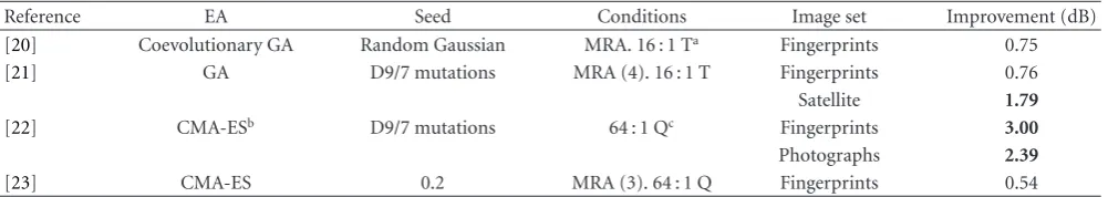
Table 1 shows the most remarkable and up to date published results in the design of wavelet transforms using Evolutionary Computation (EC), and Table 2 shows the settings of the parameters for each reported work. The authors of these works state that in the cases of MRA the coefficients evolved for each level were different, since they obtained better results using this scheme with the exception of [20].
Table1: State of the art in evolutionary wavelets design.
Reference EA Seed Conditions Image set Improvement (dB)
[20] Coevolutionary GA Random Gaussian MRA. 16 : 1 Ta Fingerprints 0.75
[21] GA D9/7 mutations MRA (4). 16 : 1 T Fingerprints 0.76
Satellite 1.79
[22] CMA-ESb D9/7 mutations 64 : 1 Qc Fingerprints 3.00
Photographs 2.39
[23] CMA-ES 0.2 MRA (3). 64 : 1 Q Fingerprints 0.54
a
Thresholding,bCovariance Matrix Adaptation-Evolution Strategy,cquantization.
Table2: Parameter settings in reported work.
Reference Parameters Platform
[20] Ga=500 Mb=150(7)c Nd=4 + 1e Intel Xeon 3 GHz
[21] G=15000 M=800 N=128 ARSCf
[22] G=?g M=? N=16 ARSC
[23] G=? M=? N=96 ARSC
a
Generations, bpopulation size, cparallel subpopulations, dindividuals
length (floating point coefficients),einteger for filter index,fArctic Region
Supercomputer Center,gunknown.
5. Proposed Simplified Evolution Strategy for an
Embedded System Implementation
As proposed in the reports by Babb, et al. [22,23], an ES was also considered within this paper scope to be the most suited algorithm to meet the requirements. However, a simpler one was chosen so that a viable hardware implementation was possible. Besides, this paper proposes, as Grasemann and Miikkulainen [20] did, the use of the LS to encode the wavelets. Therefore, it is being originally proposed here to combine both proposals from the literature so that
(i)“search algorithm”is set to be asimplifiedEvolution Strategy, and
(ii)“encoding of individuals”is done by using the Lifting Scheme.
Figure 2shows a graphical representation of the whole idea of the paper: let an evolutionary algorithm find an adequate set of parameters in order to maximize the wavelet transform performance from the compression point of view for a very specific type of images.
To reduce the computational power requirements, the whole algorithm complexity must be downscaled. This involves changing not only the parameters of the evolution but the EA itself as well. In [29] the decisions made for simplifying the algorithm as compared to the previously reported state of the art are described. These proposals, which constitute the first step in the algorithm simplification, are summarized as follows:
(1)single evolving population opposed to the parallel populations of the coevolutionary genetic algorithm proposed in [20];
sj
sj−1
dj−1
Split P U
−
+
+
p0 p1 p2 p3
P/U
stage
Delays Coefficients
Figure2: Idea of the algorithm.
(2) use ofuncorrelated mutations with one step size[13] instead of the overcomplex CMA-ES method in [22, 23];
(3) evolution ofone single set of coefficients for all MRA levels;
(4)ideal evaluation of the transform. Since doing a complete compression would turn out to be an unsustainable amount of computing time, the sim-plified evaluation method detailed in [20] was further improved. For this work, all wavelet coefficients dj are zeroed, keeping only the trend level of the transform from the last iteration of the algorithm sj, as suggested in [30]. Therefore, the evaluation of the individuals in the population is accomplished through the computation of the PSNR after setting entire bands of high-pass coefficients to 0. For 2 levels of decomposition, this is equivalent to an idealized 16 : 1 compression ratio.
solution, which means, from a phenotypic point of view, to practically discard individuals who do not concentrate efficiently most of the signal energy in the LL bands.
There were still some complex operations pending in the algorithm so the complexity relaxation was taken even further, observing always a tradeoff between performance and size of the final circuit.
(1)Uniform Random Distribution. Instead of using a Gaussian distribution for the mutation of the object parameters, a uniform distribution was tested for being simpler in terms of the HW resources needed for its implementation.
(2)Mean Absolute Error (MAE) as Evaluation Figure. PSNR is the quality measure more widely used for image processing tasks. But, as previous works in image filter design via EC show [31], using MAE gives almost identical results because the interest lies in relative comparisons among population members.
5.1. Fixed Point Arithmetic. For the implementation of the algorithm in an FPGA device, special care with binary arithmetic has to be taken since floating point representation is not hardware (FPGA) friendly. Thanks to the LS, the Integer Wavelet Transform (IWT) [32] turns up as a good solution for wavelet transforms in embedded systems. But, since filter coefficients are still represented in floating point arithmetic, a fixed point implementation is needed.
As shown in [33,34], for 8 bits per pixel (bpp) integer inputs from an image, a fixed point fractional format of Q2.10 for the lifting coefficients and a bit length in between 10 and 13 bits for a 2- to 5-level MRA transform for the partial results is enough to keep a rate-distortion performance almost equal to what is achieved with floating point arithmetic. This requires Multiply and Accumulate (MAC) units of 20–23 bits (10 bits for the fractional part of the coefficients + 10–13 bits for the partial transform results).
5.2. Modelling the Proposal. Prior to the hardware imple-mentation, modelling and extensive simulations and tests of the algorithm were done using Python computing language together with its numerical and scientific extensions, NumPy and Scipy [35], as well as the plotting library MatPlotlib [36]. Fixed point arithmetic was modelled with integer types, defining the required quantization/dequantization and bit-alignment routines to mimic hardware behaviour. Figure 3 shows the flowgraph of the algorithm.
The standard “representation” of the individuals in ESs is composed of a set ofobject parametersto be optimized and a (set of)strategy parameter(s)which determines the extent to which the object parameters are modified by the mutation operator
x1,. . .,xn,σ (1)
with xi being the coefficients of the predict and update stages. Two versions were developed, one targeting floating point numbers for the first proposal [29] and another
Initialization
Recombination
Mutation
Fitness computation
Sorting population
Create parent population
E
val
uation
Selection
Wavelet transform & compression
Figure3: Flow graph of the algorithm.
one modelling fixed point behaviour in hardware. The individuals were seeded both randomly and with the D9/7 wavelet.
The “encoding” of each wavelet individual is of the form
P1,U1,P2,U2,P3,U3,k1,k2, (2)
where each Pi and Ui consists of 4 coefficients and both kiare single coefficients. Therefore, the total length of each chromosome isn=26. As a comparison, the D9/7 wavelet is defined byP1,U1,P2,U2,k1,k2.
The “mutation” operator is defined as an uncorrelated mutation with one step size,σ. The formulae for the mutation mechanism is
σ=σ·expτ·N(0,1),
xi=xi+σ·Ni(−σ,σ),
xi=xi+σ·Ui(−σ,σ),
(3)
where N(0, 1) is a draw from the standard normal dis-tribution and Ni(−σ,σ) andUi(−σ,σ) a separate draw
from the standard normal distribution and a separate draw from the discrete uniform distribution, respectively, for each variable i (for each object parameter). The parameter τ
resembles the so-calledlearning rateof neural networks, and it is proportional to the square root of the object variable lengthn:
τ∝√1
αn, α= {1, 2}. (4)
The “fitness function” used to evaluate the offspring individuals, MAE, is defined as
MAE= 1 RC
R−1
i=0 C−1
j=0 I
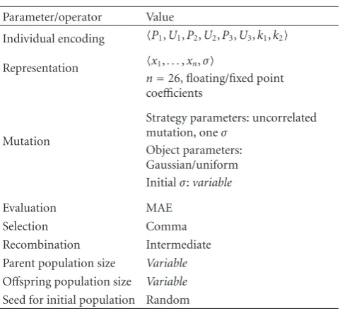
Table3: Proposed evolution strategy: summary.
Parameter/operator Value
Individual encoding P1,U1,P2,U2,P3,U3,k1,k2
Representation x1,. . .,xn,σ
n=26, floating/fixed point coefficients
Mutation
Strategy parameters: uncorrelated
mutation, oneσ
Object parameters: Gaussian/uniform Initialσ:variable
Evaluation MAE
Selection Comma
Recombination Intermediate
Parent population size Variable
Offspring population size Variable
Seed for initial population Random
where R, C are the rows and columns of the image and
I, K the original and transformed images, respectively. In previous works, the authors used PSNR for this task, but, as mentioned above, MAE produces the same results. However, for comparison purposes with other works, the evaluation of the best evolved individual against a standard image test set is reported as PSNR, computed as
MSE= 1 RC
R−1
i=0 C−1
j=0 I
i,j−Ki,j2,
PSNR=10 log10
Imax
MSE
,
(6)
where MSE stands for Mean Squared Error andImax is the
maximum possible value of a pixel, defined for B bpp as
Imax=2B−1.
For the “survivor selection”, acomma selectionmechanism has been chosen, which is generally preferred in ESs over plus selection for being, in principle, able to leave (small) local optima and not letting misadapted strategy parameters survive. Therefore, noelitismis allowed.
The “recombination” scheme chosen is intermediate recombinationwhich averages the parameters (alleles) of the selected parents.
Table 3 gathers all the information related to the pro-posed ES.
5.3. Test Strategy to Validate the Algorithm. An incremental approach has been chosen as the strategy to successively build the proposed algorithm. First of all, the complete, software-friendly implementation of the ES in floating point arithmetic was accomplished. This validated the choice of a simple ES to design new lifting wavelet filters adapted to a specific type of signal. Since the target deployment platform is an FPGA, fixed point arithmetic is desired. Therefore, the next step was to test the performance of
the fixed point implementation of the algorithm. The next great simplification to the algorithm was switching from a Gaussian-based mutation operator for the object parameters to a uniform-based one.
In order to find the best set of parameters, several tests for different combinations of them have been done in order to gather statistics of the evolutionary search performance for the training image, chosen randomly from the first set of 80 images of the FVC2000 fingerprint verification competition [37]. When changing parent population size, the offspring population size is modified accordingly to keep the selection pressure as suggested for ESs (μ/λ ≈ 1/7). Besides, the number of recombinants has been chosen to match approximately half of the population size.
The authors are aware that more tests can be performed for different settings of the parameters. Anyway, the results presented in the next section show how the proposed algorithm is widely validated within a reasonable number of computing hours (it has to be reminded here that the proposed deployment platform is an FPGA, so further tests have to be done in hardware). However, an extra test was run to check whether or not introducingelitismwas good for the evolution. The successivesimplify, test, and validatesteps are summarized as follows:
(1) begin with the SW-friendly, full precision arithmetic, simplest ES. Find a suitable initial mutation strength. Perform several tests for different values ofσ; (2) HW-friendly arithmetic implementation. Compare
with the result of (1) in fixed point arithmetic; (3) HW-friendly mutation implementation. Compare
with the result of (2) using uniform mutation; (4) repeat (1) to check whether the same initial mutation
strengths still apply after the simplifications proposed in (2) and (3);
(5) HW-friendly population size. Test the performance for different population sizes;
(6) test performance usingplusselection operator.
Tables 4, 5, 6, 7, 8, and 9 compile the information regarding the five different tests mentioned above. Please note that when the test comprises variable parameters, the number of runs shown in the table is done for each parameter value so that different, independent runs of the algorithm are executed in order to have a statistical approximation to the repeatability of the results produced.
6. Results
Table4: Test no. 1. Initial mutation stepσ.
Fixed parameters
Arithmetic Floating point
Mutation Gaussian
Population size (10/5, 70)
Variable parameters Mutation strength σ= {0.1,. . ., 2.0},Δσ=0.1
Runs 10 for each parameter variation step (total 200)
Output Performance versusσsweep
Initial mutation strengthσB? for Gaussian mutation
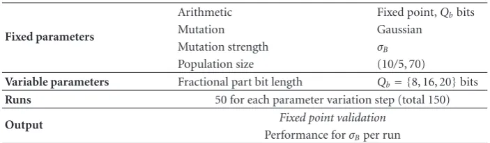
Table5: Test no. 2. Fixed point arithmetic validation.
Fixed parameters
Arithmetic Fixed point,Qbbits
Mutation Gaussian
Mutation strength σB
Population size (10/5, 70)
Variable parameters Fractional part bit length Qb= {8, 16, 20}bits
Runs 50 for each parameter variation step (total 150)
Output Fixed point validation
Performance forσBper run
Table6: Test no. 3a. Uniform mutation validation.
Fixed parameters
Arithmetic Fixed point, 16 bits
Mutation Uniform
Mutation strength σB
Population size (10/5, 70)
Runs 10
Output Uniform mutation validation
Performance for uniform mutation per run
competition. Images were black and white, sized 300×300 pixels at 500 dpi resolution. One random image was used for training and the whole set of 80 images for testing the best evolved individual in each optimization process.
Table 10shows a compilation of the figures produced during the tests. The performance for each of the standard wavelet transforms, D9/7 and D5/3, obtained with the training image is shown inTable 11.
The data collected on the boxplot figures show the statistical behaviour of the algorithm. Besides the typical values shown in this kind of graphs, all of them, likeFigure 4, show also numerical annotations for the average (top-most) and median (bottom-most) values at the top of the figure, a circle representing the average value in situ (together with the boxes) and the reference wavelets performance.
For the first step of the proposal, Test no. 1, practically all the runs (10 runs for each of the 20 σ steps, which makes a total of 200 independent runs) of the algorithm evolve towards better solutions than the standard wavelets. Statistical results of the test are included inFigure 4.
Fixed point validation which is accomplished in Test no. 2 is shown in Figure 5 forQb = {8, 16, 20} bits. 50 runs were made for eachQb value. It is clear, as expected from the comments in Section 5.1, that 8 bits for the fractional part are not enough to achieve good performance, while the
16 and 20 bits runs behave as expected. Test no. 3atries to validate uniform mutation as a valid variation operator for the EA. Good results are also obtained, as extracted from Figure 6. The only possible drawback for both tests may be the extra dispersion as compared with the original floating point implementation.
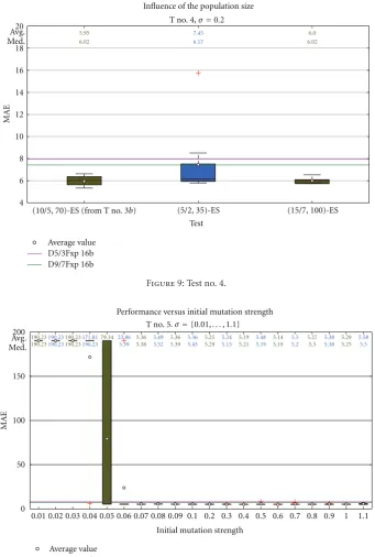
When the algorithm is simplified as in Test no. 3b, a slightly different behaviour from previous tests is observed. The most remarkable result is the difference in the perfor-mance obtained for equivalentσ values which can be seen in Figure 7. For σ ≈ {1.0,. . ., 2.0}, the dispersion of the results is very high, and a reasonable number of individuals are not evolving as expected. Therefore, the test was repeated forσ = {0.01,. . ., 0.1}, in steps of 0.01. This involves doing another 100 extra runs which are shown inFigure 8, for a total of 300 independent runs. This σ extended test range shows how the algorithm is again able to find good candidate solutions.
Results from Test no. 4 in Figure 9show the expected behaviour after changing the population size. Making it smaller as in the (5/2, 35) run does not help in keeping the average good performance of the algorithm demonstrated in previous tests for a population size of (10/5, 70). On the other hand, increasing the size to (15/5, 100) shows how the interquartile range is reduced. However, such a reduction would not justify the increase in the computational power required to evolve a 1.5 times bigger population.
The different selection mechanism chosen for Test no. 5 led to a slightly increased performance of the evolutionary search compared with Test no. 3b, as shown in Figures 10 and11.
Table7: Test no. 3b. Initial mutation stepσfor Uniform mutation.
Fixed parameters
Arithmetic Fixed point, 16 bits
Mutation Uniform
Population size (10/5, 70)
Variable parameters Mutation strength σ= {0.1,. . ., 2.0},Δσ=0.1
σa= {0.01,. . ., 0.1},Δσ=0.01
Runs 10 for each parameter variation step (total 200 + 100)
Output Performance versusσsweep
Initial mutation strengthσB? for uniform mutation
a
SeeSection 6.1for a justification of the extended range ofσ.
Table8: Test no. 4. Effect of the population size.
Fixed parameters
Arithmetic Fixed point, 16 bits
Mutation Uniform
Mutation strength σB
Variable parameters Population size (10/5, 70), (5/2, 35), (15/5, 100)
Runs 10 for each parameter variation step (total 30)
Output Performance versus population size
Table9: Test no. 5.Plusselection operator.
Fixed parameters
Arithmetic Fixed point, 16 bits
Mutation Uniform
Population size (10/5, 70)
Variable parameters Mutation strength σ= {0.01,. . ., 1.1}
Runs 10 for each parameter variation step (total 200)
Output Performance forplusselection operator versusσsweep
5.14 5.19
5.11
5.08 5.02 4.98
5.26
5.09 4.97 4.96
5.19
5.19 5.23
5.1 5.28
5.14 5.01 4.94
5.12
5.2 5.03
5.0 5.14
5.05 5.12 5.15
6.27
5.19 5.15 5.02
5.04
5.05 5.33 5.32
5.2
5.09 5.8 5.45
5.08
5.09 Performance versus initial mutation strength
0.1 0.2 0.3 0.4 0.5 0.6 0.7 0.8 0.9 1 1.1 1.2 1.3 1.4 1.5 1.6 1.7 1.8 1.9 2 Initial mutation strength
4 5 6 7 8 9 10
MAE
Avg. Med.
Average value D9/7 reference D5/3 reference
T no. 1.σ= {0.1,. . ., 2}
5.01 4.94
11.28 10.59
6.54 5.56
5.97 5.43
Test 4
6 8 10 12 14 16 18 20
MAE
Avg. Med.
Average value D9/7Fxp 8b D9/7Fxp 16b D9/7Fxp 20b
D5/3Fxp 8b D5/3Fxp 16b D5/3Fxp 20b
T no. 1 (reference test) T no. 2, 8 bits T no. 2, 16 bits T no. 2, 20 bits Fixed point validation
T no. 2 (versus T no. 1),σ=0.9
Figure5: Test no. 2.
5.79 5.52
6.66 5.67
4 6 8 10 12 14 16 18 20
MAE
Avg. Med.
Average value
Test
Uniform mutation T no. 2 (reference: Gaussian mutation)
Uniform mutation validation T no. 3a(versus T no. 2),σ=0.9
D9/7Fxp 16b D5/3Fxp 16b
Figure6: Test no. 3a.
Table10: Tests results figures.
Test no. 1 2 3a 3b 4 5
Figure 4 5 6 7,8 9 10,11
are just for the training image. Therefore, how does the best evolved individual behave for the whole test set?
Table11: Standard wavelets performance for the training image.
Wavelet D9/7 D5/3
Arithmetic Floating point Fixed point
a,Qb
Floating point Fixed point
a,Qb
8 bits 16 bits 20 bits 8 bits 16 bits 20 bits
Performance (MAE) 6.6413 7.5625 7.4190 7.4221 7.7271 7.9882 7.9595 7.9577
a
Fixed point arithmetic,Qbbits for the fractional part.
6.03 6.08
5.95 6.02
5.9 5.99
6.06 5.97
6.18 6.01
5.87 5.72
7.53 5.96
6.98 6.77
7.22 5.84
7.78 7.03
8.91 7.87
8.01 6.04
6.52 6.14
7.12 6.62
6.54 5.93
11.18 7.02
8.19 6.7
7.46 6.3
47.58 14.42
13.84 10.91
4 6 8 10 12 14 16 18 20
MAE
Avg. Med.
Average value
0.1 0.2 0.3 0.4 0.5 0.6 0.7 0.8 0.9 1 1.1 1.2 1.3 1.4 1.5 1.6 1.7 1.8 1.9 2 Initial mutation strength
Performance versus initial mutation strength T no. 3b.σ= {0.1,. . ., 2}
D9/7Fxp 16b D5/3Fxp 16b
Figure7: Test no. 3b.
24.44 6.12
6.04 6.04
6.34 6.22
6.8 6.09
6.21 6.14
6.3 6.31
6.11 6.22
6.03 6.08
6.03 6.08
5.95 6.02
5.9 5.99
6.06 5.97
6.18 6.01
5.87 5.72
7.53 5.96
6.98 6.77
7.22 5.84
7.78 7.03 98.21
190.23
4 6 8 10 12 14 16 18 20
MAE
Avg. Med.
Average value
Initial mutation strength Performance versus initial mutation strength
0.01 0.02 0.03 0.04 0.05 0.06 0.07 0.08 0.09 0.1 0.2 0.3 0.4 0.5 0.6 0.7 0.8 0.9 1
D9/7Fxp 16b D5/3Fxp 16b
T no. 3b.σ= {0.01,. . ., 1}
5.95 6.02
7.45 6.17
6.0 6.02
4 6 8 10 12 14 16 18 20
MAE
Avg. Med.
Average value
Test (10/5, 70)-ES (from T no. 3b)
T no. 4,σ=0.2
(5/2, 35)-ES (15/7, 100)-ES Influence of the population size
D9/7Fxp 16b D5/3Fxp 16b
Figure9: Test no. 4.
190.23 190.23
190.23 190.23
190.23 190.23
171.81 190.23
79.34 5.51
23.86 5.39
5.36 5.38
5.49 5.52
5.36 5.39
5.36 5.43
5.25 5.29
5.24 5.15
5.19 5.21
5.48 5.19
5.14 5.19
5.5 5.2
5.27 5.3
5.38 5.38
5.29 5.25
5.58 5.5
MAE
Avg. Med.
Average value
Initial mutation strength Performance versus initial mutation strength
= {0.01,. . ., 1.1} T no. 5. σ
0.01 0.02 0.03 0.04 0.05 0.06 0.07 0.08 0.09 0.1 0.2 0.3 0.4 0.5 0.6 0.7 0.8 0.9 1 1.1 0
50 100 150 200
D9/7Fxp 16b D5/3Fxp 16b
Figure10: Test no. 5.σ= {0.01,. . ., 1.0}.
sets of results will assist in the validation of the successive simplifications made to the originally proposed algorithm.
Figure 12 shows a graph of the evolution run of the best individual for the whole set of tests for floating point arithmetic and Gaussian mutation and fixed point arithmetic and uniform mutation for both,commaandplusselection, respectively. Thebestindividual has been chosen as the one averaging the highest performance against the whole test set (not the one performing best for the training image, as is
190.23 190.23
190.23
190.23
190.23 190.23
171.81
190.23
79.34 5.51
23.86
5.39
5.36 5.38
5.49
5.52
5.36 5.39
5.36
5.43
5.25 5.29
5.24
5.15
5.19 5.21
5.48
5.19
5.14 5.19
5.5
5.2
5.27 5.3
5.38
5.38
5.29 5.25
5.58
5.5
MAE
Avg. Med.
Average value
Initial mutation strength Performance versus initial mutation strength
0.01 0.02 0.03 0.04 0.05 0.06 0.07 0.08 0.09 0.1 0.2 0.3 0.4 0.5 0.6 0.7 0.8 0.9 1 1.1 4
5 6 7 8 9 10
D9/7Fxp 16b D5/3Fxp 16b
= {0.01,. . ., 1.1} T no. 5. σ
Figure11: Test no. 5. Zoom-in inFigure 10.
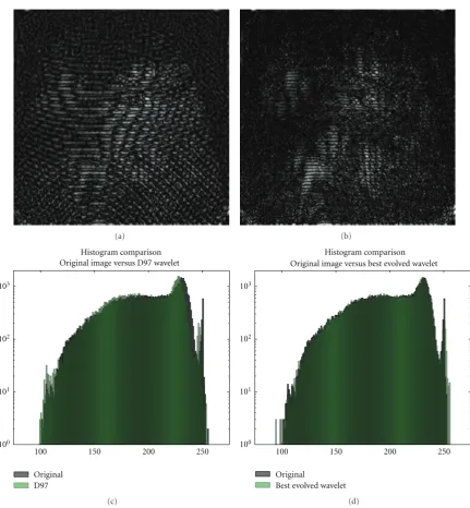
judgement, though some artifacts are clearly visible in the performance of the D9/7 wavelet as shown inFigure 16(c). It can be seen from these error images and histograms how, after applying aforward transform + (ideal) compression + inverse transformto an image, the result of using the evolved wavelet generates an image which keeps a higher degree of similarity with the original one than using the standard D9/7.
6.3. Some Comments on Results. Section 5.3 featured a discussion on the design validation followed to obtain a hardware-friendly ES by successively simplifying a previously validated and much more complex algorithm. Various inde-pendent test runs have been performed to look for the best setting of parameters, beginning with a software-friendly, high-precision floating point arithmetic version which used Gaussian mutations. After simplifying the algorithm and validating each of the steps, several conclusions can be extracted.
Because of its usual influence in EAs, search for an adequate mutation rate (mutation strength in ESs) has enjoyed a particular computing effort. It can be said, however, that, for this particular optimization problem, the mutation strength is not critical, as long as it belongs to a reasonable range. Outside of that range, evolution is not able to find good candidate solutions. Table 12shows the most suitable range of values found for σ, chosen as those runs resulting in average performance values behaving better than the standard wavelets.
The whole set of tests have validated the proposal and found a reasonably good set of parameters for the problem at hand which is
(i) fixed point arithmetic,Qb=16 bits,
Table12: Initial mutation strength range.
Conditions Values
Floating point, Gaussian mutation σ= {0.1,. . ., 2.0}
Fixed point, uniform mutation,comma
selection σ= {0.03,. . ., 0.6}
Fixed point, uniform mutation,plusselection σ= {0.07,. . ., 1.1}
(ii) population sizes: (10/5, 70),
(iii) selection operator with elitism:plusselection,
(iv) uniform mutation with an initial mutation step contained within the range shown inTable 12.
As can be observed inFigure 12the algorithm stagnates soon in every single run, around generation 200 for the floating point and Gaussian mutation runs and generation 160 for fixed point uniform mutation and comma selection. In the floating point case, the stagnation is not complete because it keeps on improving very slowly, but in practical terms it does not imply a substantial improvement in the quality of the transform. Although the best individuals keep on stagnating if elitism is introduced in the evolution, the worst ones still maintain some degree of variation, improving the overall algorithm performance as compared to the nonelitist strategy.
0 200 400 600 800 1000 Generations
0 10 20 30 40 50
Best fit Worst fit Average fit
Fit
ness
(MAE)
D97 fit D53 fit
(a)
0 200 400 600 800 1000
Generations 0
10 20 30 40 50
Best fit Worst fit Average fit
Fit
n
ess
(MAE)
D97Fxp fit D53Fxp fit
(b)
0 200 400 600 800 1000
Generations 0
10 20 30 40 50
Best fit Worst fit Average fit
Fit
n
ess
(MAE)
D97Fxp fit D53Fxp fit
(c)
Figure12: Best evolution run for (a) floating point arithmetic and Gaussian mutation; (b) fixed point arithmetic and uniform mutation, comma selection; (c) fixed point arithmetic and uniform mutation, plus selection.
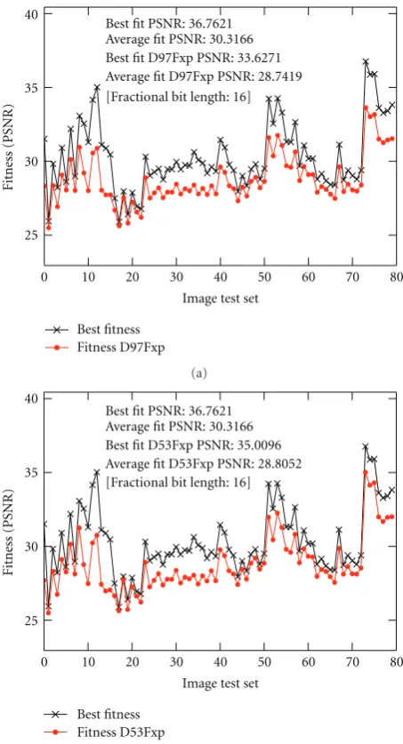
were originally developed for this task (optimizing real-valued vectors). Compared with [22], where the best evolved wavelet outperforms the reference wavelet by 3.00 dB, the performance versus complexity tradeoff in the algorithm proposed in this paper achieves a good 1.57 dB improvement, which corresponds to the 30.31 dB performance against the whole test set as shown in Figure 15. Besides, it should be noted that for all the runs (140) corresponding to theσrange shown inTable 12 for Test no. 5, the average performance obtained was 29.76 dB, where only 4 out of the whole 140 runs were not able to improve existing wavelets.
Table13: Comparison of best evolved wavelet against state of the art.
Reference EA Seed Improvement
over D9/7 (dB)
[20] Coevolutionary
GA Random Gaussian 0.75
[21] GA D9/7 + mutations 0.76
[22] CMA-ES D9/7 + mutations 3.00
This paper ES Random Gaussian 1.57a
a
0 10 20 30 40 50 60 70 80 Image test set
25 30 35 40
Fit
n
ess
(PSNR)
Best fit PSNR: 36.9672 Average fit PSNR: 30.3668 Best fit D53 PSNR: 36.2053 Average fit D53 PSNR: 29.0977
Best fitness Fitness D53
(a) Best fit PSNR: 36.9672 Average fit PSNR: 30.3668 Best fit D97 PSNR: 36.6231 Average fit D97 PSNR: 29.5990
0 10 20 30 40 50 60 70 80 Image test set
25 30 35 40
Fit
n
ess
(PSNR)
Best fitness Fitness D97
(b)
Figure13: Performance of the best evolved individual for Floating point arithmetic and Gaussian mutation against the whole test set: (a) for D5/3 and (b) for D9/7 wavelets.
7. Hardware Implementation
7.1. Architecture Mapping. HW/SW Partitioning. Typical implementations of evolutionary optimization engines in FPGAs place the EA in an embedded processor. With this approach, some degree of performance is sacrificed to gain flexibility in the system (needed to fine tune the algorithm), so that modifications may be easily done to the (software) implementation of the EA (which is, of course, much easier than changing its hardware counterpart).Table 14shows the partitioning resulting from applying this design philosophy. According to Algorithm 1, each of the EA operators are shown in the table together with further actions to be accom-plished: recombination (of the selected parents), mutation (of the recombinant individuals to build up a new offspring
Best fit PSNR: 36.8523 Average fit PSNR: 30.1985 Best fit D97Fxp PSNR: 33.6271 Average fit D97Fxp PSNR: 28.7419 [Fractional bit length: 16]
0 10 20 30 40 50 60 70 80 Image test set
25 30 35 40
Fit
n
ess
(PSNR)
Best fitness Fitness D97Fxp
(a) Best fit PSNR: 36.8523 Average fit PSNR: 30.1985 Best fit D53Fxp PSNR: 35.0096 Average fit D53Fxp PSNR: 28.8052 [Fractional bit length: 16]
0 10 20 30 40 50 60 70 80 Image test set
25 30 35 40
Fit
n
ess
(PSNR)
Best fitness Fitness D53Fxp
(b)
Figure 14: Performance of the best evolved individual for fixed
point arithmetic and uniform mutation (commaselection) against
the whole test set: (a) comparison with D9/7 and (b) comparison with D5/3 wavelets.
Table14: HW/SW partitioning of the system.
EA operator Further actions HW SW
Recombination — √
Mutation — √
Evaluation Wavelet transform
√
Fitness computation √
Selection Sorting population
√
Create parent population √
population), evaluation (of each offspring individual), and selection(of the new parent population).
Best fit PSNR: 36.7621 Average fit PSNR: 30.3166 Best fit D97Fxp PSNR: 33.6271 Average fit D97Fxp PSNR: 28.7419 [Fractional bit length: 16]
0 10 20 30 40 50 60 70 80 Image test set
25 30 35 40
Fit
n
ess
(PSNR)
Best fitness Fitness D97Fxp
(a) Best fit PSNR: 36.7621 Average fit PSNR: 30.3166 Best fit D53Fxp PSNR: 35.0096 Average fit D53Fxp PSNR: 28.8052 [Fractional bit length: 16]
0 10 20 30 40 50 60 70 80 Image test set
25 30 35 40
Fit
n
ess
(PSNR)
Best fitness Fitness D53Fxp
(b)
Figure 15: Performance of the best evolved individual for fixed point arithmetic and uniform mutation (plusselection) against the whole test set: (a) comparison with D9/7 and (b) comparison with D5/3 wavelets.
responsible for its evaluation. This comprises the compu-tation of the fitness as the Mean Absolute Error (MAE) as shown in (5). To tackle it, the following sequence of operations has to be done: Forward Wavelet Transform (fWT), Compression (C), Inverse Wavelet Transform (iWT) (wavelet transform), and MAE figure computation (fitness computation). Once each offspring individual has been evalu-ated, the population is sorted according to the result (sorting population). At this stage, the microprocessor may close the evolutionary loop creating the new parent population. Afterwards, recombination and mutation are applied, and a new offspring population will be available for evaluation.
Figure 18 shows the proposed conceptual architecture capable of hosting such a system. The functions which have
(a)
(b)
(c)
Figure16: Transform performance. (a) Original fingerprint image; comparison of the performance obtained with (b) D9/7 fixed point implementation and (c) best evolved individual.
been implemented in hardware work as attached peripherals to the microprocessor embedded in the FPGA (PowerPC 440).
(a) (b)
100 101 102 103
Histogram comparison
Original D97
100 150 200 250
Original image versus D97 wavelet
(c)
Histogram comparison
Original 100
101 102 103
100 150 200 250
Best evolved wavelet
Original image versus best evolved wavelet
(d)
Figure17: Transform performance. The top row shows the error introduced by each transform: (a) is the error image for the D97 wavelet and (b) for the best evolved individual. The bottom row shows the histograms of each image transform, where: (c) is for D97 and (d) for the best evolved individual.
Taking advantage of the LS features, the fWT and iWT can be computed by just doing a sign flip and a reversal in the order of the operations (PandUstages), so both modules are sharing hardware resources in the FPGA. The Compression block is simple, since it only needs to substitute the fWT result by zeros for each datum of the details bands. Therefore, it works in parallel with the fWT. In a similar manner, the Fitness module computes the difference image as each pixel is produced by the iWT.
The fWT/iWT module is built up by applying the sequence of P, U stages dictated by the LS. To mimic the high-level modelling of the algorithm (seeSection 5.2), 6 stages have been implemented (3P and 3U), each one
containing 4 filter coefficients which is enough to implement the most common wavelets utilized at present. Section 7.3 shows the first preliminary results of the implementation. The implementation of each P,U stage can be seen in Figure 19.
μP interface BRAM functionFitness
Population sorting
BU
S
Flash memory
μP
FPGA (Virtex 5 FX70T) iWT
fWT Compression
Figure18: System level architecture.
Dela
ys
Coefficients
Even
P(even)
Odd
Odd − +
+
+
+
Figure19: Predict/Update stage implementation.
the four sub-banks is used for the actual image being tested, and the other three are loaded with the following test images in the meantime, acting as a multi-ping-pong memory.
7.2. HW/SW Partitioning Validation. The model developed to validate the algorithm has been profiled.Table 15shows profiling results for 500 generations for each EA operator. Table 14 is repeated (for clarity) adding extra columns with the result values. Absolute values are not of real interest (although NumPy routines are highly optimized, a C implementation would be faster), since what is being checked is the relative amount of time spent in each phase so that design partitioning is validated as a whole. As expected, most of the time is consumed evaluating the individuals. In each generation, 20.479 ms (=1433.56/(500 generations ∗ 70 individuals ∗ 2 transforms)) are needed to compute a single wavelet transform, whether it is a forward or an inverse one. The obtained results validate the design partitioning proposed except for the selection operator, which is low enough to be implemented in SW. The reason to choose an HW implementation for it is that it can be applied as results are produced by the fitness computation module, saving extra time. In contrast, the simulation of the Python model runs on a single processor thread. Therefore, all operators are applied sequentially. But in the hardware implementation, some operators can be easily applied in parallel. For this reason, and depending on the scope of the system (see Section 8), some other operator will probably benefit from
Table15: Algorithm code profiling.
EA operator Further actions HW SW Timea %
Recombination — √ 0.14 0.009
Mutation — √ 0.43 0.029
Evaluation
Wavelet transformb √ 1433.56 97.470
Compression √ 4.96 0.337
Fitness computation √ 31.62 2.150
Selection Sorting population
√
0.040 0.003
Parent population √
a
All results in seconds.
bResults show computation time for both, forward and inverse wavelet
transform.
being implemented in hardware, as, for example, the muta-tion. Besides, the subset of the C language used to program the PowerPC processor in the FPGA imposes restrictions that will probably cause the percentage of the time each operator takes to compute to increase.
7.3. Preliminary Hardware Implementation Results. The pro-totype platform selected is an ML507 development board, which contains a Xilinx Virtex 5 XC5VFX70T FPGA device with an embedded PowerPC processor, responsible for running the ES.Table 16 shows the preliminary implemen-tation results for an overdimensioned datapath of 32 bits, using 16 bits for the fractional part representation. This implementation is directed towards a system level functional validation in the FPGA, giving higher area results than expected for the final system.
The current hardware, nonoptimized implementation, delivers one result each clock cycle. For a 256×256 pixels image, with a clock frequency of 100 MHz, the computation time of a wavelet transform is approximately 0.65 ms. This is a speedup factor of around (20.5/0.65) 31 times, which would turn into 45 seconds to do all the transforms required by a population of 70 individuals during 500 generations.
8. Conclusion and Future Work
A bio-inspired optimization algorithm designed to improve wavelet transform for image compression in embedded systems has been proposed and validated. A simpler method than the standard ES (and simpler than other previously evolutionary-based reported works) has been developed to find a suitable set of lifting filter coefficients to be used in the aforementioned wavelet transformation. Fixed point arithmetic implementation has been used to validate the upcoming hardware implementation.
Table16: Preliminary implementation results for the main modules in the system.
Module Resources Frequency (MHz)
Slice LUTs Slice registers DSP48Es BRAM (Kb)
fWT/iWT 3077/44800 3905/44800 62/128 — 147
Compression 35/44800 31/44800 — — 426
Fitness function 74/44800 60/44800 — — 348
Population sorting 2913/44800 2140/44800 — — 233
Image memory 333/44800 20/44800 — 2304/5328 —
When the final implementation of the system in the FPGA is finished and tested, profiling results will be obtained. This is necessary due to the possible effect that the C language subset used to program the PowerPC processor in the FPGA may have, which could impose restrictions that will probably cause the percentage of time each operator takes to compute to increase drastically. For example, if this was the case for the uniform mutation operator (which will initially be implemented in SW), further simplifications to this operator could be tested as suggested for ESs in the lit-erature. Anyway, since the algorithm finds a solution around generation 200, it can be said, being on the conservative side, that, if 500 generations are needed to evolve, just 45 seconds would elapse for the most time-consuming task, making this a sufficiently fast adaptive system.
The current status of this paper shows how adaptive compression for embedded systems based on bio-inspired algorithms can be looked at. Besides, since the process is sped-up by a large factor in the hardware implementation as compared to the software, PC-based model, the system can also be conceived as an accelerator for the optimization process of wavelet transforms (for the construction of custom wavelets).
For a generic vision system as in the one mentioned in the Introduction, this paper allows for the fact that both approximations toadaptationmentioned inSection 4can be combined, firstly defining a new set of wavelets adapted to a specific type of signals (covered by this paper) and, during system operation, using some of the proposed methods in the literature that may help the system to further adapt to local changes in the signal. However, it can be said that, if the EA has been successful and the training data set properly chosen, there should not be a drastic improvement, since the EA should have acquired enough knowledge of that specific type of signal. Moreover, in a hypothetical continuously evolving system, a mechanism that looks for reductions of performance (EA kept running on the background) can be implemented and triggered to keep on evolving the wavelet if relevant changes happen in the input signal (some of them probably caused by a degradation in the sensing devices that diminish the acquired signal quality).
Acknowledgments
This work was supported by the Spanish Ministry of Science and Research under the project DR.SIMON
(Dynamic Reconfigurability for Scalability in Multimedia-Oriented Networks) with TEC2008-06486-C02-01. L. Sekan-ina has been supported by MSMT under research program MSM0021630528 and by the Grant of the Czech Science Foundation GP103/10/1517. Rub´en Salvador would like to thank the support received from the Department of Computer Systems, Brno University of Technology, during his research stay as part of his PhD degree.
References
[1] W. Sweldens, “The lifting scheme: a custom-design
construc-tion of biorthogonal wavelets,” Applied and Computational
Harmonic Analysis, vol. 3, no. 2, pp. 186–200, 1996.
[2] D. Taubman and M. Marcellin,JPEG2000: Image Compression
Fundamentals, Standards and Practice, Springer, 1st edition, 2001.
[3] W. MacLean, “An evaluation of the suitability of FPGAs
for embedded vision systems,” in Proceedings of the IEEE
Computer Society Conference on Computer Vision and Pattern Recognition (CVPR ’05), p. 131, June 2005.
[4] B. Cope, P. Y. K. Cheung, W. Luk, and S. Witt, “Have GPUs made FPGAs redundant in the field of Video Processing?” inProceedings of the IEEE International Conference on Field Programmable Technology, pp. 111–118, December 2005.
[5] S. Che, J. Li, J. W. Sheaffer, K. Skadron, and J. Lach,
“Accelerating compute-intensive applications with GPUs and
FPGAs,” in Proceedings of the Symposium on Application
Specific Processors (SASP ’08), pp. 101–107, June 2008. [6] Z. Wei, D.-J. Lee, B. E. Nelson, J. K. Archibald, and B. B.
Edwards, “FPGA-based embedded motion estimation sensor,”
International Journal of Reconfigurable Computing, vol. 2008, no. 636145, p. 8, 2008.
[7] C. Farabet, C. Poulet, and Y. LeCun, “An FPGA-based stream processor for embedded real-time vision with convolutional
networks,” in Proceedings of the IEEE 12th International
Conference on Computer Vision Workshops (ICCV ’09), pp. 878–885, September 2009.
[8] B. Jawerth and W. Sweldens, “Overview of wavelet based
multiresolution analyses,”SIAM Review, vol. 36, no. 3, pp.
377–412, 1994.
[9] S. Mallat,A Wavelet Tour of Signal Processing, Academic Press, 2nd edition, 1999.
[10] W. Sweldens, “The lifting scheme: a construction of second
generation wavelets,”SIAM Journal on Mathematical Analysis,
vol. 29, no. 2, pp. 511–546, 1998.
[11] W. Sweldens, “The lifting scheme: a new philosophy in
biorthogonal wavelet constructions,” inWavelet Applications
[12] A. Eiben and J. Smith,Introduction to Evolutionary Computing, Springer, 2008.
[13] H. Beyer and H. Schwefel, “Evolution strategies. A
compre-hensive introduction,”Natural Computing, vol. 1, no. 1, pp.
3–52, 2002.
[14] N. Hansen, “The CMA evolution strategy: a comparing
review,” inTowards a New Evolutionary Computation, pp. 75–
102, 2006.
[15] R. R. Coifman and M. V. Wickerhauser, “Entropy-based
algorithms for best basis selection,” IEEE Transactions on
Information Theory, vol. 38, no. 2, pp. 713–718, 1992. [16] S. G. Mallat and Z. Zhang, “Matching pursuits with
time-frequency dictionaries,”IEEE Transactions on Signal
Process-ing, vol. 41, no. 12, pp. 3397–3415, 1993.
[17] M. M. Lankhorst and M. D. van der Laan, “Wavelet-based
sig-nal approximation with genetic algorithms,” inEvolutionary
Programming, pp. 237–255, 1995.
[18] R. L. Claypoole, R. G. Baraniuk, and R. D. Nowak, “Adaptive wavelet transforms via lifting,” inProceedings of the IEEE Inter-national Conference on Acoustics, Speech and Signal Processing, pp. 1513–1516, May 1998.
[19] G. Piella and H. J. A. M. Heijmans, “Adaptive lifting schemes
with perfect reconstruction,” IEEE Transactions on Signal
Processing, vol. 50, no. 7, pp. 1620–1630, 2002.
[20] U. Grasemann and R. Miikkulainen, “Effective image
com-pression using evolved wavelets,” inProceedings of the Confer-ence on Genetic and Evolutionary Computation (GECCO ’05), pp. 1961–1968, ACM, New York, NY, USA, 2005.
[21] B. Babb and F. Moore, “The best fingerprint compression stan-dard yet,” inProceedings of the IEEE International Conference on Systems, Man, and Cybernetics (SMC ’07), pp. 2911–2916, October 2007.
[22] B. Babb, F. Moore, M. Peterson, T. H. O’Donnell, M. Blowers, and K. L. Priddy, “Optimized satellite image compression and
reconstruction via evolution strategies,” inEvolutionary and
Bio-Inspired Computation: Theory and Applications III, vol. 7347, Orlando, Fla, USA, May 2009, 73470O.
[23] B. J. Babb, F. W. Moore, and M. R. Peterson, “Improved multiresolution analysis transforms for satellite image com-pression and reconstruction using evolution strategies,” in
Proceedings of the 11th Annual Conference Companion on Genetic and Evolutionary Computation Conference: Late Break-ing Papers, pp. 2547–2552, ACM, Montreal, Canada, 2009.
[24] F. Moore and B. Babb, “A differential evolution algorithm
for optimizing signal compression and reconstruction
trans-forms,” inProceedings of the Conference Companion on Genetic
and Evolutionary Computation (GECCO ’05), pp. 1907–1912, ACM, Atlanta, Ga, USA, 2008.
[25] F. Moore, P. Marshall, and E. Balster, “Evolved transforms for
image reconstruction,” inProceedings of the IEEE Congress on
Evolutionary Computation, vol. 3, pp. 2310–2316, September 2005.
[26] B. Babb, S. Becke, and F. Moore, “Evolving optimized matched forward and inverse transform pairs via genetic algorithms,” in
Proceedings of the IEEE International 48th Midwest Symposium on Circuits and Systems (MWSCAS ’05), vol. 2, pp. 1055–1058, August 2005.
[27] F. Moore, “A genetic algorithm for evolving multi-resolution analysis transforms,”WSEAS Transactions on Signal Processing, vol. 1, pp. 97–104, 2005.
[28] F. Moore and B. Babb, “Revolutionary image compression and reconstruction via evolutionary computation, part 2: multiresolution analysis transforms,” inProceedings of the 6th
WSEAS International Conference on Signal, Speech and Image Processing, pp. 144–149, World Scientific and Engineering Academy and Society (WSEAS), Lisbon, Portugal, 2006. [29] R. Salvador, F. Moreno, T. Riesgo, and L. Sekanina,
“Evolu-tionary design and optimization of wavelet transforms for
image compression in embedded systems,” inProceedings of
the NASA/ESA Conference on Adaptive Hardware and Systems (AHS ’10), pp. 171–178, IEEE Computer Society, June 2010. [30] J. D. Villasenor, B. Belzer, and J. Liao, “Wavelet filter evaluation
for image compression,”IEEE Transactions on Image
Process-ing, vol. 4, no. 8, pp. 1053–1060, 1995.
[31] Z. Vasicek and L. Sekanina, “An evolvable hardware system in
Xilinx Virtex II Pro FPGA,”International Journal of Computer
Application, vol. 1, no. 1, pp. 63–73, 2007.
[32] A. R. Calderbank, I. Daubechies, W. Sweldens, and B. L. Yeo,
“Wavelet transforms that map integers to integers,”Applied
and Computational Harmonic Analysis, vol. 5, no. 3, pp. 332– 369, 1998.
[33] M. Martina, G. Masera, G. Piccinini, and M. Zamboni, “A VLSI architecture for IWT (Integer Wavelet Transform),” in
Proceedings of the 43rd IEEE Midwest Symposium on Circuits and Systems, vol. 3, pp. 1174–1177, August 2000.
[34] M. Grangetto, E. Magli, M. Martina, and G. Olmo, “Optimiza-tion and implementa“Optimiza-tion of the integer wavelet transform for image coding,”IEEE Transactions on Image Processing, vol. 11, no. 6, pp. 596–604, 2002.
[35] T. E. Oliphant, “Python for scientific computing,”Computing
in Science and Engineering, vol. 9, no. 3, Article ID 4160250, pp. 10–20, 2007.
[36] J. D. Hunter, “Matplotlib: a 2D graphics environment,”
Computing in Science and Engineering, vol. 9, no. 3, Article ID 4160265, pp. 99–104, 2007.
[37] D. Maio, D. Maltoni, R. Cappelli, J. L. Wayman, and A. K.
Jain, “FVC2000: fingerprint verification competition,” IEEE