Volume 2006, Article ID 36971, Pages1–16 DOI 10.1155/ASP/2006/36971
Super-Resolution Using Hidden Markov Model and
Bayesian Detection Estimation Framework
Fabrice Humblot1, 2and Ali Mohammad-Djafari2
1DGA/DET/SCET/CEP/ASC/GIP, 94114 Arcueil, France
2LSS/UMR8506 (CNRS-Sup´elec-UPS), 91192 Gif-sur-Yvette Cedex, France
Received 12 December 2004; Revised 22 May 2005; Accepted 27 May 2005
This paper presents a new method for super-resolution (SR) reconstruction of a high-resolution (HR) image from several low-resolution (LR) images. The HR image is assumed to be composed of homogeneous regions. Thus, the a priori distribution of the pixels is modeled by a finite mixture model (FMM) and a Potts Markov model (PMM) for the labels. The whole a priori model is then a hierarchical Markov model. The LR images are assumed to be obtained from the HR image by lowpass filtering, arbitrarily translation, decimation, and finally corruption by a random noise. The problem is then put in a Bayesian detection and estimation framework, and appropriate algorithms are developed based on Markov chain Monte Carlo (MCMC) Gibbs sampling. At the end, we have not only an estimate of the HR image but also an estimate of the classification labels which leads to a segmentation result. Copyright © 2006 F. Humblot and A. Mohammad-Djafari. This is an open access article distributed under the Creative Commons Attribution License, which permits unrestricted use, distribution, and reproduction in any medium, provided the original work is properly cited.
1. INTRODUCTION
This paper concerns super-resolution (SR) reconstruction of an image from a few low-resolution (LR) images in order to gain a better detection on faintly contrasted and isolated specks having a size of almost one pixel in a picture. In this paper we deal more particularly with the SR process.
The SR reconstruction consists in producing a high-resolution (HR) image from a set of LR images. These LR images can be taken from a video sequence. They must come out from a moving scene:the movement and nonredundant information are what make SR process possible. So, the ob-tained HR picture contains more useful information than one of the LR pictures taken in the initial video sequence.
One of the main steps in a SR reconstruction process is the registration of the different LR images. It is defined as the way of matching two or more pictures showing the same scene from different viewpoints, from different sensors, or at different times. To get a good SR reconstruction, it is es-sential to know accurately the transformation that enables to go from one LR picture to another. Our work context allows us to limit the field of possible transformations between two pictures to the global translatory motion. Indeed, it does not seem unrealistic to have a stabilized and controlled camera to obtain the initial LR video sequence. We can imagine that the movement of the camera during the image acquisition
is limited to global translational move, and that there is no zoom effect (equivalent to homothety transformation) and no rotation of the camera axis. To deal with this problem, we use the image registration by phase correlation. This method and its extension using the gradients of the images are well explained in [1,2]. We also evaluated both methods in our previous work [3]. These methods are interesting for the eas-iness of their implementation, the speed of their execution on a computer, and their good subpixel accuracy.
SR methods may be categorized into two main divi-sions: frequency domain and spatial domain techniques. Our proposed methods use the linear spatial domain observa-tion model. They are stochastic methods, and they use the Bayesian framework. Other works used the same Bayesian approach, we can cite for instance [4,5].
The problem of SR has been addressed for the first time in [6], with a frequency domain approach. It would be too long to describe all the different SR approaches, so we suggest [7,8] that give very good overviews of them.
(MAP) framework. Gaussian MRF priors are well known to produce overly smoothed restorations. The Tikhonov reg-ularization approach is a special case of the more gen-eral Bayesian framework under the assumptions of Gaussian noise and prior.
Many works are based basically on modeling the link be-tween the LR images and the HR image through a lowpass filtering, decimating, and translation movement. This is also the model we choose. But to our knowledge, all the existing HR reconstruction methods are based either on a least square estimation which leads to an interpolation, registration, and summation [13], or at the best, on the regularization ap-proach [9–12]. Here, we propose a Bayesian estimation framework which gives the possibility to account for a wider class of a priori model for the distribution of the pixels of the HR image. The method we propose here assumes that the HR image is composed of homogeneous regions. Thus, the a pri-ori distribution of the pixels is modeled by a finite mixture model (FMM) to let their classification in a finite number of classes, and a Potts Markov model (PMM) for the labels. The FMM is a common tool for classification, but in general, the discrete variable which represents the classes is assumed to be i.i.d. Our Potts Markov model for these variables gives the possibility to account for spatial correlation of the pixels. In fact, the PMM parameter controls the mean value of the size of the agglomerated pixels in different classes and thus the mean value of the segmented regions in the image.
The method proposed in [4] concerns the image restora-tion using Gauss-Markov random fields and line process. Our work differs from that work in two main aspects. First, the purpose of that work is an image restoration which is conceptually different of SR methods. Next, authors of this paper use a line process where we use a label process. More, the novelty of our work in comparison to all known meth-ods is that our framework allows us to obtain not only an estimate of the HR image, but also an estimate of the classi-fication labels which leads to a segmentation result. This last result is useful for possible geometrical features estimation of the results, for example, for a tracking of feature in satellite images. The Bayesian probabilistic framework gives a good estimation of the real classification of the scene.
The authors in [5] consider the SR problem and use a classical approach, also used for instance in [12]. More specifically, in this article, authors focus on an estimation stage of the SR parameters. Our method differs from this work in the model relating the LR images to HR image which is not exactly the same, and in the prior modeling of the HR image which is a Markov and not a compound Gauss-Markov random fields, with hidden label process.
In summary, the proposed a priori model for the distri-bution of the pixels of the HR image results in a hierarchical Markov model which gives the possibility to estimate jointly the HR image, the classification labels which can be used as a segmentation result and also the parameters of the a priori, and the noise model which results in a totally unsupervised HR image estimation and segmentation.
Indeed, the hierarchical structure of the model can be appropriately implemented using the Markov chain Monte Carlo (MCMC) Gibbs sampling.
The paper is organized as follows: inSection 2, the for-ward model linking the HR image to LR images is detailed, and the basics of the Bayesian estimation framework for SR reconstruction is presented. InSection 3, we give the details of the a priori models for the HR image pixels distribution which is composed of a FMM and Potts MRF. InSection 4, we give the expressions of all the posterior laws which are necessary for the implementation of the MCMC Gibbs sam-pling. InSection 5, we give details of implemented MCMC Gibbs sampling algorithm. InSection 6, we first present the results which we can obtain with the proposed method and then compare its performances with a classical interpola-tion, registrainterpola-tion, and summation [13], and with another classical method based on popular Tikhonov regularized ap-proach [9].Section 7shows results obtained with real video sequences. Finally, we present conclusions and perspectives of this work inSection 8.
2. FORWARD MODEL AND THE BAYESIAN ESTIMATION FOR SR RECONSTRUCTION
A simple model which links the LR images and the HR image is
gi=DMiBf+i=Hif+i, i=1,. . .,M, (1)
where f is the HR image, {gi,i=1,...,M} represent the M LR images,Brepresents the lowpass filter operator needed be-fore sampling a HR image,Miare operators representing the translation movements,Drepresents a decimation operator, iare the additive noises representing all the errors, and fi-nally,Hi=DMiBrepresents the composite operator linking the HR imagefto the LR imagegi. This is the forward model. Noting thatgi,i, andfrepresent the images, we also note them bygi(r),i(r), and f(r), wherer=(x,y)∈N2 repre-sents the pixel position, andgi(r) = [DMiBf](r) +i(r), whereB,Mi, andDare respectively the equivalent contin-uous operators ofB,Mi, andD.
Note that we may use the following combination:
g= ⎡ ⎢ ⎢ ⎣
g1 .. . gM
⎤ ⎥ ⎥
⎦, H= ⎡ ⎢ ⎢ ⎣
H1 .. . HM
⎤ ⎥ ⎥
⎦, = ⎡ ⎢ ⎢ ⎣
1 .. . M
⎤ ⎥ ⎥ ⎦ (2)
to rewrite (1) as
g=Hf+, (3)
where, given f andH, computingg is the forward model, and estimatingf, givenHandg, is the corresponding inverse problem. The direct problem is to obtain the LR images from a HR image.
f
gi
fi
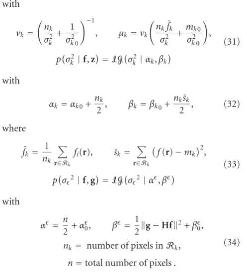
Figure1: HR imagef, LR imagesgi=DMif,i=1,. . ., 4, registered
and interpolated imagesfi=MtiDtgi, which can be used to obtain a HR image by a classical method consisting inf=(1/M) ifi.
represents a HR image, each symbol representing a different pixel of the image. The second shows a representation of all the LR images obtained from the previous HR image and for a decimation factord=2. Finally, all the registered and inter-polated LR pictures on the HR grid can be seen on the third and last row. The symbols with full contours are the original pixel values from LR images, and symbols with dotted con-tours are interpolated pixel values.
Next, the fact of taking one pixel over two in the original HR image to create the LR images shows the effect of oper-atorDfor a decimation factord=2. And the fact that two neighboring pixels of the HR image, for instance, the upper-left circle and diamond, are located at the same position in the corresponding LR images (the upper-left pixel) shows the effect of operatorsMi. Thus, the second row shows how to go fromftogi,i=1,...,4.
Lastly, the presence of interpolated pixels values on the third row of Figure 1 shows the inverse effect of operator D. And the fact that the upper-left circle and diamond have found back their correct initial positions (in comparison to their positions in the initial HR image) shows the inverse ef-fect of operatorMi.
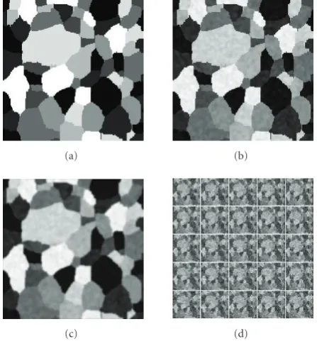
Through an example of size 125×125 pixels2,Figure 2 shows the forward process of generation of LR images from a HR image f that can be seen on image (a). It starts by a lowpass filtering, givingBf shown on (b), sampling, trans-lation, and decimation by a factord of 5 giveHf and it is shown on (c), and finally, alteration by a random noise repre-senting measurement noise and all the other errors of mod-eling givesg, which is shown on (d) (we used a noise cen-tered, white, and Gaussian obtained with a SNR—see (35)— of 5 dB).
The Bayesian estimation framework for SR reconstruc-tion can be summarized as follows.
(i) Use the forward model (1) and some assumptions on the noise to obtain the likelihood p(g | f,θ), where θ represents the parameters of the probability distri-bution of the noise.
(a) (b)
(c) (d)
Figure2: (a) A HR imagef, (b) its lowpass filteredBf, (c) LR
im-ages without noisegi=Hif, and (d) LR images with additive noise
gi=Hif+i.
(ii) Use all the prior information or the desired properties for the solution to assign an a priori probability distri-butionp(f|θf), whereθf is its parameters.
(iii) Use the Bayesian approach to obtain
(a) the a posteriori probability distribution
pf|g,θ∝pg|f,θpf|θf
, (4)
where θ = (θ,θf) if θ is known (supervised case), or
(b) the joint a posteriori probability distribution
pf,θ|g∝pg|f,θpf|θf
p(θf)p(θ) (5)
if theθis unknown (unsupervised case).
(iv) Finally, define an estimatorfforf, andθforθ, based on these posterior probability laws.
The next section defines more in detail the prior laws which are needed to obtain the expressions of these posterior laws, and proposes different estimators based on them.
3. A PRIORI MODEL OF THE HR IMAGE PIXELS
3.1. HMM modeling of HR image
hidden Markov modeling (HMM) is a very general and ef-ficient way to model appropriately such images. The main idea is to assume that all the pixel values fk of a homoge-neous regionkfollow a given probability law, for example, a GaussianN(mk1,Σk), where1is a generic vector of ones of sizenk = |Rk|which is the number of pixels in regionk with knk= |R| =n, the total number of pixels of the HR image.
In the following, we consider two cases.
(i) The pixels in a given region are assumed i.i.d.:
pf(r)|z(r)=k=Nf(r)|mk,σk
, k=1,. . .,K, (6)
and thus
pfk
=pf(r),r∈Rk=Nfk|mk1,σk2I
, (7)
withIthe identity matrix of sizenk.
(ii) The pixels in a given region are assumed to be locally dependent:
pfk
=pf(r), r∈Rk=Nfk|mk1,Σk
, (8)
where Σk is an appropriate covariance matrix whose shape and structure depend on the modeling of this dependency. We propose a first-order Markov model with the four nearest neighbors.
In both cases, the pixels in different regions are assumed to be independent:
pf|z= K
k=1 pfk
=
K
k=1
Nfk|mk1,Σk
. (9)
Note that f(r) is a scalar and p(f(r) | z(r) = k) is its conditional probability density function, butfk is a vector andp(fk) is the joint probability density function of all the pixels in regionk.
3.2. Modeling the labels
Noting that the two models (7) and (8) are conditioned on the value ofz(r)=k, they can be rewritten in the following general form:
pfk(r)
= K
k=1
Pz(r)=kNfk(r)|mk,σk2
. (10)
Now, we need also to model the probability distribution P(Z(r) = z(r), r ∈ R) of the vector random variables Z = {Z(r) :r∈R}which we note hereafterp(z). For this too, we consider two cases.
(i) Independent Gaussian mixture (IGM) model, where {Z(r), r∈R}are assumed to be independent and
Pz(r)=k=pk,
with K
k=1
pk=1, p(z)= K
k=1 pk.
(11)
(ii) Contextual Gaussian mixture (CGM) model that we also call hidden Markov model (HMM), where{Z(r), r ∈ R}are assumed to be Markovian:
p(z)∝exp
α
r∈R
s∈V(r)
δz(r)−z(s)
, (12)
which is the Potts Markov random field (PMRF).V(r) rep-resents neighboring pixels ofswith|V(r)| =4. The Marko-vian modeling with a connexity of 4 considers that each label value z(r) of a pixel at position ris function of the values of its four closest pixelsz(s),s∈V(r) (neighboring pixels). They are the one above, the one on its right, the one under, and the one on its left. The parameterαcontrols the mean value of the regions’ sizes. Here, it controls the mean value of the sizes of the classes, that is, increasingαresults in a realiza-tion where the different classes become more homogeneous. Using the Hammerslay-Clifford equivalence of the Gibbs and Markov random fields, we can also write
pz(r)|z(s),s∈R∝exp
α
s∈V(r)
δz(r)−z(s)
(13)
which shows that the probability of obtaining a labelz(r) for a pixel is related to the number of neighboring pixels hav-ing the same label. We remind thatδ(·) is the Dirac function defined byδ(0)=1, andδ(t)=0 fort=0.
3.3. Hyperparameters prior law
The final point before obtaining an expression for the poste-rior probability law of all the unknowns, that is, p(f,θ |g) is to assign a prior probability lawp(θ) to the hyperparam-eters θ. Even if this point has been one of the main dis-cussing points between Bayesian and classical statistical re-search community, and still there are many open problems, we choose here to use the conjugate priors for simplicity. The conjugate priors have at least two advantages:
(i) they can be considered as a particular family of a dif-ferential geometry-based family of priors [14–16], (ii) and they are easy to use because the prior and the
pos-terior probability laws stay in the same family.
In our case, we need to assign prior probability laws to the meansmk, to the variancesσk2or to the covariance matrices
Σk, and also to the covariance matrices of the noisesΣi. The conjugate priors for the meansmkare, in general, the GaussiansN(mk|mk0,σk20), those of variancesσk2are the in-verse GammasIG(σ2
k |αk0,βk0), and those for the covariance matricesΣkare the inverse Wishart’sIW(Σk|αk0,Λk0). See the appendix for a detailed expression of these probability density functions.
4. A POSTERIORI PROBABILITY LAWS
(i) Likelihood.
The expression of the likelihood depends on the observa-tion model (1). Then, the expression is
pg|f,θ= M
i=1
pgi|f,Σi
= M
i=1
Ngi|Hif,Σi
,
(14)
where we assumed that the noisesi are independent, cen-tered, and Gaussian with covariance matrices Σi which, hereafter, are also assumed to be diagonalΣi = σ2iI. We noteθ= {σ2i, i=1,. . .,M}.
(ii) HMM for the images:
pf|z,θf
= K
k=1
pfk|mk1,Σk
= K
k=1
Nfk|mk1,Σk
,
(15)
whereΣk is characterized either byσk2assuming Σk = σk2I, or by an extra parameterρk which controls the correlation between the neighboring pixels. Assuming that the pixels in a homogeneous region are modeled with a homogeneous Gauss-Markov field,
pfk
∝exp ⎡
⎣
r∈Rk
f(r)−β(r)
s∈V(r) f(s)
2⎤
⎦ (16)
considering the four nearest pixels neighborhood.
Thus, here, the hyperparameters becomeθf = {(mk,σk2, ρk), k=1,. . .,K}.
(iii) PMRF for the labels:
p(z)∝exp
α
r∈R
s∈V(r)
δz(r)−z(s)
, (17)
where we used the simplified notation p(z) = P(Z(r) = z(r), r∈R).
(iv) Conjugate priors for the hyperparameters:
pmk
=Nmk|mk0,σk20
,
pσ2 k
=IGσ2
k |αk0,βk0
,
pΣk
=IWΣk|αk0,Λk0
,
pσ2i
=IGσ2i |α0i,β0i
.
(18)
(v) Joint posterior law off,z, andθ:
pf,z,θ|g∝pg|f,θpf|z,θf
p(z)p(θ). (19)
The forward model and the priors for this case can be summarized as follows:
gi=Hif+i←→g=Hf+,
pg|f=Ng|Hf,Σ withΣ=diagΣ1,. . .,ΣM
,
pgi|f
=Ngi|Hif,Σi
withΣi=σ2iI,
pf(r)|z(r)=k=Nf(r)|mk,σk2
, k=1,. . .,K,
Rk=r:z(r)=k, fk=
f(r) :r∈Rk,
pfk
=Nfk|mk1k,Σk
withΣk=σk2Ik,
p(z)=pz(r), r∈R∝exp
α
r∈R
s∈V(r)
δz(r)−z(s)
,
pf|z= k
Nfk|mk1k,Σk
=Nf|mz,Σz
,
withmz=[m111,. . .,mk1K
, Σz=diag
Σ1,. . .,ΣK
,
pmk
=Nmk|mk0,σk20
,
pσk2
=IGσk2|αk0,βk0
,
pσ2=IGσ2|α 0,β0
.
(20)
5. MAXIMUM A POSTERIORI AND MCMC GIBBS SAMPLING
5.1. Maximum a posteriori
First, assume thatθ andz are known. Then, consider the maximum a posteriori (MAP) estimate
f=arg max
f
pf|g,z,θ=arg min
f
Jf|g,z,θ. (21)
Then, it is easy to show that
(i) when pixels in given regions are assumed to be i.i.d. (7), we have
J1
f|g,z,θ= g−Hf 2+λ f−m 2Σ
= g−Hf 2+λ(f−m)tΣ−1(f−m)
= M
i=1
gi−Hif2 +λ
K
k=1
fk−mk12 σk2
= M
i=1
gi−Hif2 +λ
K
k=1
r∈Rk
f(r)−mk2 σ2
k ,
(22)
where we noted byΣ2=diag[σ2
(ii) when pixels in given regions are assumed to be locally dependent (8) with a local Markovian model, we have
J2
f|g,z,θ
= g−Hf 2+λ f−m 2
Σ
= g−Hf 2+λ(f−m)tΣ−1(f−m)
= g−Hf 2+λD(f−m)2
= M
i=1
gi−Hif2 +λ
K
k=1 D˜fk2
σk2
= M
i=1
gi−Hif2
+λ K
k=1 1 σ2 k
r∈Rk
˜ f(r)−βr
s∈(V(r)∩Rk) ˜ f(s)
2 ,
(23)
where Σ−1 = diag [σ2
1,. . .,σK2]DDt, ˜f(r) = f(r)− m(r), andβra coefficient depending on pixelr. Letnr
be Card(V(r)∩Rk), which is the number of neighbor-ing pixels of the pixelrthat belong to the same region Rk.βrequals to 1/nrifnr =0 and equals to 0
other-wise.
Note that, when we assume that the whole image is com-posed of one statistically homogeneous region (K=1), these two criteria become
J1(f)= g−Hf 2+ λ
σ2 f−m 2,
J2(f)= g−Hf 2+ λ
σ2D(f−m) 2
,
(24)
which can then be compared to the regularization criterion used by [9]. It is the classical Tikhonov regularization ap-proach withoutσ2andm, values that we get from our classi-fication.
So, compared to the classical regularization methods and, in particular, the SR method firstly proposed by [9], here, we go farther in details of modeling the HR image. Indeed, we model the HR image as to be a piecewise homogeneous regions, each characterized by a Gaussian process with mean mk, varianceσk2, or covarianceΣk. In the last case, we assume a Gauss-Markov process with the four nearest neighbors.
5.2. MCMC Gibbs sampling
One more advantage with this model is that we also can go farther and try to estimate both the shape of each homo-geneous region modeled throughz(r) and estimate also the corresponding hyperparametersmkandσk2through an iter-ative process (unsupervised) using either any alternate opti-mization such as Expectation-Maxiopti-mization or a more gen-eral MCMC Gibbs sampling process. For this purpose, we propose the following general iterative algorithms.
(i) Joint MAP (Algorithm 1):
f=arg max
f
pf|z,θ,g,
θ=arg max
θ
pθ|f,z,g,
z=arg max
z
pz|f,θ,g.
(25)
(ii) MAP-Gibbs sampling (Algorithm 2):
f=arg max
f
pf|z,θ,g,
sampleθusingpθ|f,z,g,
samplezusingpz|f,θ,g,
or usingpz|θ,g,
(26)
or still
(ii) MAP-Gibbs sampling (Algorithm 3):
f=arg max
f
pf|z,θ,g,
θ=arg max
θ
pθ|f,z,g,
samplezusingpz|f,θ,g,
or usingpz|θ,g.
(27)
In all cases, we need to initialize the algorithm. For this, we propose to start by assuming K = 1, and thusz = 1 and θ = [m1,σ12] = [0, 1]. This means that we try to obtain a regularized solutionf(0)from which we can use any classical histogram-based segmentation to obtainz(0), and a classical maximum likelihood estimation approach to obtain a first estimationθ(0)forθ. Then, we can continue the iterations using any of the proposed algorithms.
Between the three proposed algorithms, we may note that there is not any theoretical guaranty of the conver-gence for either of them. However, in Algorithms 1 and 3, the critical point in the segmentation part is to compute
θ = arg maxθp(θ|f,z,g), because it can give values ofσk which are very small (10−6or even less) if pixels of a region Rk have almost all the same values. This difficulty is atten-uated in Algorithm 2, which is the one we used for all our simulations.
The following relations summarize all the posterior prob-ability laws that are needed to implement these algorithms:
pf|z,θ,g=Nf|f,Σ (28)
with
Σ=HtΣ
−1H+Σz−1 −1
, f=ΣHtΣ
−1g+Σz−1mz
,
pz|g,θ∝pg|z,θp(z)
(29)
with
pg|z,θ=Ng|Hmz,Σg
withΣg=HΣzHt+Σ,
pmk|z,f
=Nmk|μk,vk
with
vk=
nk σ2 k
+ 1 σ2 k0
−1
, μk=vk
nkf¯k σ2
k +mk0
σ2 k0
,
pσ2 k |f,z
=IGσ2 k |αk,βk
(31)
with
αk=αk0+nk
2, βk=βk0+ nks¯k
2 , (32)
where
¯ fk=
1 nk
r∈Rk
fi(r), s¯k=
r∈Rk
f(r)−mk 2
,
pσ2|f,g=IGσ2|α,β
(33)
with
α=n 2 +α
0, β= 1 2 g−Hf
2+β 0,
nk= number of pixels inRk,
n=total number of pixels.
(34)
Some details about the way we obtained these relations are given in the appendix.
6. SIMULATION RESULTS AND PERFORMANCES OF THE PROPOSED METHOD WITH ARTIFICIALLY GENERATED LR IMAGES
To have a good evaluation of this new method, and for the evaluation of its performances, we constructed our own LR pictures from a supposed HR image of size 125×125 pixels2. Because of the classification feature of our technique that leads to a segmentation of the HR image, we began this con-struction with a segmented picture composed of only two labels. It is made of two circles, two rectangles, and two squares. This picture constitutes our reference segmented imagez0and can be seen onFigure 3(a). Letn(r) be a noise, we define here the signal-to-noise ratio (SNR) in dB as fol-lows:
SNR=10×log10
r∈Rf(r) +n(r) 2
r∈Rn(r)2
. (35)
Our idea about this construction is to start from a known discrete-value imagez0 representing the labels of homoge-neous regions in the image and shown onFigure 3(a), and simulate a HR imagef. For this step, we generated a colored noise with a SNR of 20.5 dB and added it toz0 to obtain f. We used this image, which can be seen on Figure 3(b), as our reference HR image f0. Then we apply the forward transformation equation (1), applying first a 5×5 Gaussian kernel lowpass filter B to f0. Resulting image is shown on
Figure 3(c). We choose a decimation factord = 5, and we constructM = d2 = 25 LR images using the scheme illus-trated onFigure 1in the cased=2. Thus, we are in an ideal
(a) (b)
(c) (d)
Figure3: (a)z0to obtain HR imagef0, (b) HR imagef0, (c) lowpass
filtered imageBf0, and (d) noisy LR imagesgi=Hif0+i.
case where we can observeMdifferent LR imagesgishowing different views of a same HR imagef0. These LR images can be seen onFigure 2(c). Finally we add to each LR imagegi in-dependently a centered, white and Gaussian noise, obtained for a SNR of 5 dB. These LR noisy images, which constitute our simulated data, are onFigure 3(d). This choice of value for the noise parameters was a way of showing the robustness of our method in noise conditions. If it is working quite well with hard noise conditions, it will be working too with less noise.
We used the gradient phase correlation method that we evaluated in [3] for the registration process. For this ideal case, and without noise (Figure 2(c)), the registration process gives an accurate estimation of the shifts between all LR pic-tures. These information, and for a given interpolation factor d, allow to register and interpolate linearly pixel values on the HR grid. This step is illustrated on the second and third lines ofFigure 1. We can also use one or two reference images to fill the unknown areas (e.g., the first and the last registered and interpolated LR pictures).
For the noisy case, the registration method does not give the same accuracy in the estimation of movement between LR images. The registration method evaluates correctly 28% of all shifts between pictures. For 30% of them, the wrong values were very close (±1/d) to the exact move values.
For the choice of parameters and hyperparameters, we choose the PMRF parameterαequals to 2 in all the following simulations of our methods. We normalize all the original HR imagesf0between 0 and 1, and we choose for allk:mk0= 0.5,σ2
k0=0.1,αk0=α0=1, andβk0=β0=2.
(a) (b)
(c) (d)
Figure4: (a)fmean, (b)fmedian, (c)fTikhonov 1,λ=1, and (d)fTikhonov 2,
λ=1.
(a) (b)
Figure5: Results of segmentationz3(a), and reconstructed HR
im-agef3(b) withK=3 and forλ=1, when pixels in given regions
are assumed to be i.i.d.
model (11). Concerning the three algorithms presented in Section 5.2, we used Algorithm 2 with MAP-Gibbs sampling which provided us the better results. Algorithm 3 was partic-ularly critical because, at that stage of our works, we imposed the number of classes to use in the segmentation part. So, a class becoming unrepresented can give aσk2very close to zero, making (22) or (23) to explode.
We compared the performances of our method with two other SR schemes. The first one uses a registration, a classi-cal linear interpolation, and a summation [13]. Iffiare the LR imagesgiregistered and interpolated, we have fmean(r)= (1/M) Mi=1fi(r). On the same model, we can also replace the median of pixels instead of the mean giving fmedian(r). The second one is another classical method based on popu-lar Tikhonov regupopu-larized approach [9–12]. This method is a deterministic approach utilizing regularization functions
(a) (b)
(c) (d)
Figure6: Results of segmentationz3withK=3 (a) and (c), and
reconstructed HR imagef3(b) and (d), respectively, forλ=10 and
λ=102, when pixels in given regions are assumed to be locally
de-pendent.
to impose smoothness constraints on the space of feasible solutions. We implemented two versions of this method:
fTikhonov1, where we use classical derivative highpass kernel operator of size 3×3 to computeDf.fTikhonov2is almost the same thing, except that it adaptsDfor the pixels located on the corner of the pictures.
We define evaluation criteria using the difference im-age Δ between our reference HR image f0 and any HR image f reconstructed from our noisy LR images gi. We used the estimation of the shifts obtained from these im-ages. Thus, Δ(f,f0) = f −f0. We also define Δα(f,f0) =
r∈R|Δ(f(r),f0(r))|α/ r∈R|f0(r)|α, forα= {1, 2}, as be-ing L1 and L2 normalized relative error measures.
Because of our choice of HR image, which have regions with frank discontinuities, it seems more interesting to look at Δ1(f,f0). So, for each case, we computed Δ1, the mean (which is the bias of our HR estimator) and standard devi-ation of the difference imageΔ(f,f0):ΔmeanandΔSD. More-over, for our methods, we will give percentage of error onz label estimation.
We first experimented our method with a synthetical im-age obtained from a segmented imim-age using 2 labels only. Figure 4shows the results obtained forfmean(a),fmedian(b),
Table1: Synthetic image made of 2 labels: evaluation criteria of SR methods.
Methods Δmean(×10−2) ΔSD Δ1(×10−1) Error on estimation
of labels (%)
Mean of pixel values,fmean 0.74 0.125 3.36 ×
Median of pixel values,fmedian 0.63 0.124 3.40 ×
fTikhonov 1,λ=1 0.67 0.117 3.56 ×
fTikhonov 2,λ=1 0.06 0.128 4.24 ×
(f3,z3), i.i.d.,λ=1 0.41 0.105 2.04 9.09
(f3,z3), dependent,λ=10 1.03 0.134 3.45 7.17
(f3,z3), dependent,λ=102 3.86 0.118 3.31 7.58
(f2,z2), dependent,λ=10 3.35 0.135 2.80 2.67
(a) (b)
Figure7: Results of segmentationz2(a), and reconstructed HR
im-agef2(b) withK=2 and forλ=10, when pixels in given regions
are assumed to be locally dependent.
regions and using (8) and (23). (a) and (b) show respectively
zandf, forλ=10 andK=3. (c) and (d) show respectively
zandf, forλ =102 andK =3.Figure 7shows the results obtained in the same case, but for only two labels. Thus, (a) and (b) show respectivelyzandf, forλ=10 andK=2.
Table 1presents the values of our evaluation criteria for all the previous cases shown on Figures4,5,6, and7. Firstly, it is important to remind that our method is stochastic. So, another realization of our algorithm can give some other, but close, results. Next, our methods give a piece of information that usual methods do not give: a segmented imagez. This knowledge about the HR image could be useful to a detection purpose. It is also useful to the reconstruction of the HR im-age. If we look at all these different reconstructed HR images
f, it seems that our method considering a local dependency between pixels of the same region, withK =3,λ=102, and shown onFigure 6(d), highlights the contours of the shapes. These contours seem to be more sharp and contrasted with our methods than for the other compared methods. Indeed, the methods of comparison give images without sharp edges, but with blurred object’s contours. Also, our method allows to distinguish the squares from the circles.
For our methods, on the point of view of the percentage of error on labels’ estimation, it is not surprising to have less errors when we use 2 labels than when we use more labels since we made our original HR image from 2 labels.
(a) (b)
(c) (d)
Figure8: (a)z0to obtain HR imagef0, (b) HR imagef0, (c) lowpass
filtered imageBf0, and (d) noisy LR imagesgi=Hif0+i.
We can also notice that our reconstruction seems ro-bust to error of the estimation of the movement since we use an estimated movement vector which included errors. Fi-nally, we remark that no one of our chosen criteria seems to be adapted to evaluate the quality of the reconstructed HR picture.
(a) (b)
(c) (d)
Figure9: (a)fmean, (b)fmedian, (c)fTikhonov 1,λ=1, and (d)fTikhonov 2,
λ=1.
(a) (b)
(c) (d)
Figure10: Results of segmentationz8withK=8 (a) and (c), and
reconstructed HR imagef8(b) and (d), respectively, for pixels
as-sumed to be i.i.d. andλ=1, and for pixels assumed to be locally dependent andλ=103.
Here again, our method that considers a local depen-dency between pixels of the same region, withK = 3 and λ=103, gives a better reconstructed HR image if we look at the homogeneity of regions and their sharp contours.
Finally, we did the same experiment on a real image of size 250×250 pixels2 taken from the sky, and that can be seen onFigure 11(b). We did a segmentation of this picture withK = 8 labels and used evenly distributed thresholds. It is shown on (a) of the same figure. Except for the colored noise that we did not add, we constructed our own LR images as before. The blurred imageBf0is onFigure 11(c), and the noisyM =25 LR pictures, with a noise of 5 dB, can be seen onFigure 11(d). The registration method evaluates correctly 28% of all shifts between noisy pictures. All the results of the used methods are shown on Figures12and13.Table 3gives the evaluation criteria values.
For this real and more detailed HR image, our method that assumes pixels are i.i.d.,K =8,λ = 1, and shown on Figure 13(b), seems to give a good reconstruction of the ini-tial HR imagef.
7. SIMULATION RESULTS OBTAINED WITH REAL VIDEO SEQUENCES
We used a Philips ToUCam Video WebCam to obtain three real video sequences. For each case, we used a super-resolution factor ofd=4. First, we did a 208 frames movie usingFigure 14(a)as the main image of the video sequence. The registration process found all the 16 over 16 possible subpixel moves in all the frames of the sequence.Figure 14(b) shows one of the 38×64 pixels2 LR real frames we used to compute HR images, (c) is thefmeansolution, and (d) is the
fTikhonov2withλ=1 solution.
Figure 15(a)shows the result of segmentationz2, and (b) the reconstructed HR imagef2when we use our method with K = 2 andλ = 10−1. (c) shows the result of segmentation
z3, and (b) the reconstructed HR imagef3when we use our method withK=3 andλ=10−1.
The HR images obtained with our method are quite similar to the one obtained with the two other methods. However, if we look closely, it appears that object’s con-tours are more accurate with our method (Figures15(b)and 15(d)). Indeed, we also have the segmented images (a) and (c) ofFigure 15that show more precisely the object’s forms, in particular, image (c) which is the segmentation’s result when we use 3 labels.
The second movie is filmed using Figure 16(a) as the main image of the video sequence. The registration process found 14 over 16 possible subpixel moves in the 120 frames of the sequence.Figure 16(b)shows one of the 53×57 pixels2 LR real frames we used to compute HR images, (c) is thefmean solution, and (d) is thefTikhonov2withλ=1 solution.
Figure 17(a)shows the result of segmentationz3, and (b) the reconstructed HR imagef3when we use our method with K = 3 andλ = 10−1. (c) shows the result of segmentation
z7, and (b) the reconstructed HR imagef7when we use our method withK=7 andλ=10−1.
Table2: Synthetic image using 8 labels: evaluation criteria of SR methods.
Methods Δmean(×10−2) ΔSD Δ1(×10−1) Error on estimation
of labels (%)
Mean of pixel values,fmean 0.14 0.108 1.33 ×
Median of pixel values,fmedian 0.21 0.110 1.35 ×
fTikhonov 1,λ=1 0.34 0.114 1.48 ×
fTikhonov 2,λ=10 1.85 0.108 1.48 ×
(f8,z8), i.i.d.,λ=1 4.54 0.132 2.03 32.7
(f8,z8), dependent,λ=103 8.16 0.155 2.82 29.7
(a) (b)
(c) (d)
Figure11: (a)z0obtained by thresholding of the HR imagef0and
K =8 labels, (b) HR imagef0, (c) lowpass filtered imageBf0, and
(d) noisy LR imagesgi=Hif0+i.
image (c) which is the segmentation’s result when we use 7 labels.
The last video sequence is made of 313 frames. The reg-istration process found all the 16 over 16 possible subpixel moves in all the frames of the sequence.Figure 18(b)shows one of the 70×69 pixels2LR real frames we used to compute HR images, (c) is thefmeansolution, and (d) is thefTikhonov2 withλ=1 solution.
Figure 19(a)shows the result of segmentationz3, and (b) the reconstructed HR imagef3when we use our method with K = 3 andλ = 10−2. (c) shows the result of segmentation
z6, and (b) the reconstructed HR imagef6when we use our method withK=6 andλ=10−2.
This last video, showing more complicated real images, allows to see that our method works well. For example, the text “ PHILIPS” on both batteries can be clearly read on the HR images obtained with our method (Figures 19(b)
(a) (b)
(c) (d)
Figure 12: (a) fmean, (b) fmedian, (c)fTikhonov 1, λ = 1, and (d)
fTikhonov 2,λ=1.
and 19(d)), but it is not so clear on the HR images ob-tained with other methods. Even the time on the digital clock can be read on the HR images obtained with our method, which is not the case on the other HR images. More, the segmentation’s result shown on images (a) and (c) of Figure 19allows to have information about the dif-ferent homogeneous regions of the HR image, which is not the case for the HR images obtained with the other meth-ods.
From a computational point of view, our methods are more expensive in comparison to classical methods pre-sented in this work. Indeed, in each main iteration of the algorithm we have chosen inSection 5.2, we have 3 steps:
Table3: Image taken from the sky: evaluation criteria of SR methods.
Methods Δmean(×10−2) ΔSD Δ1(×10−1) Error on estimation
of labels (%)
Mean of pixel values,fmean 0.24 0.104 1.41 ×
Median of pixel values,fmedian 0.27 0.106 1.44 ×
fTikhonov 1,λ=1 0.26 0.113 1.48 ×
fTikhonov 2,λ=1 0.20 0.102 1.44 ×
(f8,z8), i.i.d.,λ=1 0.90 0.117 1.61 13.0
(f8,z8), dependent,λ=103 8.76 0.122 2.27 13.8
(a) (b)
(c) (d)
Figure13: Results of segmentationz8withK=8 (a) and (c), and
reconstructed HR imagef8(b) and (d), respectively, for pixels
as-sumed to be i.i.d. andλ=1, and for pixels assumed to be locally dependent andλ=103.
(2) sampling ofzwhich is not really too expensive, mainly the cost of the computation of a forward problem, (3) sampling of hyperparameters which is not expensive
neither, mainly the cost of computation of the means and variances of the pixel values in each region.
More precisely, if we letXandYbe the size of LR images in pixels (width and height),Mthe number of LR images used in the SR process,K the number of labels used for the seg-mentation of the HR imagefK, anddthe SR factor, then the calculation complexity of methods givingfmeanandfmedianis O(X,Y,M,d2). It is the same complexity whenf
Tikhonov 1and
fTikhonov 2 are computed, even if an iterative process is per-formed.
For our methods, the calculation complexity isO(X,Y, M,d2,K). However, it is not easy to give an exact compara-tive cost computation. For this reason, we performed some experimental time comparison using the CPU time for the execution of these different methods.Table 4gives the com-putation times (in seconds) we obtained using Matlab, on a Windows XP OS, with a Pentium IV processor at 2.6 GHz. We did these time estimations for the clock real sequence (whose results are shown on Figures18and19), and the arti-ficially generated sequence showing a view of the earth took from the sky (results shown on Figures12and13).Table 4 also gives in each case the overall number of iterations real-ized to obtainfin the full optimization process (first number between brackets), and the number of iterations done in our SR methods (second number between brackets). The two last lines of this table show that, with the absolute same condi-tions, the number of iterations in our algorithm can be very different, even if the obtained results are almost the same. This is due to the probabilistic approach of our methods.
We first noticed that there is a multiplicative factor rang-ing between 5 and 10 as regards the necessary comput-ing time between the computation time of classical method
fTikhonov 2and our method giving (fK,zK). More, we can also see that the computational time needed to obtain the final result is a function of the number of iteration realized.
8. CONCLUSION
(a) (b)
(c) (d)
Figure14: (a) Image used to obtain the video sequence, (b) one
LR image (38×64 pixels2), (c)f
mean(152×256 pixels2), and (d)
fTikhonov 2,λ=1.
the problem through a global Gibbs sampling scheme. One aspect of the originality of our work concerns the different kind of results we obtain with our stochastic SR method: we do not only obtain a reconstructed HR imagef, but also a segmented imagezwhich can be useful for geometrical fea-ture extraction and their tracking.
The perspectives of our future works on SR reconstruc-tion methods are to first apply these methods on more plex real video sequences. Also, we want to use a more com-plete movement scheme to estimate the affine motion be-tween LR images, including homothety and rotation. The au-thors of [18] propose such a more sophisticated movement model. Finally, we may also look to an adaptation of our SR methods for color images.
For now, the number of labels used in the segmentation process must be fixed. So, another research axis could con-cern an automated and clever evolution of the number of necessary labels to obtain the best reconstructed HR picture. To end, it would be interesting to find a good evaluation criterion that will permit to characterize a good HR recon-structed image.
APPENDIX
A. EXPRESSIONS OF THE PRIOR PROBABILITY LAWS MENTIONED INSECTION 3.3
Nmk|mk0,σk20
= 1 2πσ2
k0 exp
−1
2
mk−mk0 σk0
2 ,
Nfk|mk1,Σk
= Σk 1/2
(2π)nk/2exp
−1
2
fk−mk1 t
Σ−1 k
fk−mk1
,
(A.1)
withnkthe number of pixels offthat belong to the region
(a) (b)
(c) (d)
Figure15: (a) Results of segmentationz2and (b) reconstructed HR
imagef2withK =2 andλ=10−1, (c) results of segmentationz3
and (d) reconstructed HR imagef3withK=3 andλ=10−1.
Rk,|Σk|the determinant of the matrixΣk, and1a vector of sizenkwith all components equal to 1.
IGσk2|α,β
=Γβα (α)
1 σk2
α−1 exp
−β1
σk2
,
IWΣk|α,Λ
=|Λ|α Γ(α)
Σk 1−α
exp−ΛΣ−k1
.
(A.2)
B. EXPRESSIONS OF THE POSTERIOR PROBABILITY LAWS MENTIONED IN SECTIONS5.1AND5.2
(i) Posterior law off|z,θ,g:
pf|z,θ,g∝pg|f,z,θpf|z,θ
∝Ng|f,σ2 I
K
k=1
pfk|zk,θ
∝Ng|Hf,σ2 I
K
k=1
Nfk|mk1,σk2Ik
∝Ng|Hf,σ2 I
Nf|mz,Σz
∝Nf|f,Σ,
(B.1)
withΣ=(HtΣ
−1H+Σz−1)−1, andf =Σ(HtΣ−1g+ Σz−1mz), and wheremz is a vector of the size of the image defined asmz =[m111,. . .,mk1K], and where
Σz = diag[Σ1,. . .,ΣK].1k is a vector of sizenk with all components equal to 1, andΣkis a diagonal matrix withσ2
kas its diagonal elements. (ii) Posterior laws ofz|f,θ,g, andz|g,θ:
pz|f,θ,g∝pg|f,z,θp(z)
∝Ng|Hf,σ2 I
p(z),
pz|g,θ∝pg|z,θp(z)
∝Ng|Hmz,HΣzHt+Σp(z).
(a) (b) (c) (d)
Figure16: (a) Image used to obtain the video sequence, (b) one LR image (53×57 pixels2), (c)f
mean(212×228 pixels2), and (d)fTikhonov2,
λ=1.
(a) (b) (c) (d)
Figure17: (a) Results of segmentationz3and (b) reconstructed HR imagef3withK=3 andλ=10−1, (c) results of segmentationz7and
(d) reconstructed HR imagef7withK=7 andλ=10−1.
(a) (b) (c)
Figure18: (a) One LR image (70×69 pixels2), (b)f
mean(280×276 pixels2), and (c)fTikhonov 2,λ=1.
(a) (b) (c) (d)
Figure19: (a) Results of segmentationz3and (b) reconstructed HR imagef3withK=3 andλ=10−2, (c) results of segmentationz6and
Table4: Computation times (in seconds) and number of iterations (to computef, in the iterative algorithm) obtained using different SR methods.
Methods
Clock sequence (Figures18,19) View from sky (Figures12,13) (X,Y,M,d)=(70, 69, 16, 4) (X,Y,M,d)=(50, 49, 13, 4) Computation time Iterations (No.) Computation time Iterations (No.) [2pt] Mean of pixel values,fmean 6.3 (×,×) 3.0 (×,×)
Median of pixel values,fmedian 15.6 (×,×) 7.5 (×,×)
fTikhonov 2,λ=1 8.1 (26,×) 3.2 (24,×)
(f3,z3), i.i.d.,λ=10−3 22.0 (41, 17) 8.1 (37, 11)
(f6,z6), i.i.d.,λ=10−3 24.3 (36, 12) 11.4 (37, 11)
(f3,z3), dependent,λ=10−2 42.2 (41, 16) 13.6 (34, 6)
(f6,z6), dependent,λ=10−2 32.0 (29, 4) 20.4 (36, 6)
(f6,z6), dependent,λ=10−2 53.0 (38, 13) 30.0 (44, 14)
(iii) Posterior laws ofθ|z,f,g:
pθ|z,f,g
= M
i=1
pσ2i |f,gi K
k=1
pmk|σk2,f,z
pσk2|mk,f,z
,
pmk|σk2,f,z
∝pf|mk,σk2,z
pmk|σk2,z
∝Nfk|mk1,σk2I
×Nmk|mk0,σk02
∼Nmk|mapostk0 ,σk02 apost ∝ 1 2πσ2 k nk/2
exp
− 1 2σ2
k
fk−mk12
× 1 2πσk02
exp
− 1 2σk02
mk−mk02 ,
δ pmk|σk2,f,zb
δmk =0=⇒
1 σk2
r∈Rk
f(r) +mk0 σk02
=mk nk σ2 k + 1 σ2 k0 , σ2 k0 apost = nk σ2 k + 1 σ2 k0 −1 ,
mapostk0 =σk02 apost
1 σk2
r∈Rk
f(r) +mk0 σk02
,
pσ2
k |mk,f,z
∝pf|σk2,mk,z
pσk2|mk,z
∝Nfk|mk1,σk2I
×IGσ2
k |αk0,βk0
∼IGσ2 k
apost
|αapostk0 ,βapostk0
∝
1 2πσ2
k nk/2
exp
− 1 2σ2
k
fk−mk12
(B.3)
×
1 σk2
αk0−1 exp
−βk0
1 σk2
∝
1 σk2
αk0+(nk/2)−1 exp
−1
σk2
βk0+
fk−mk12 2
,
αk0apost=αk0+nk 2,
βk0apost=βk0+1 2
r∈Rk
f(r)−mk2 ,
pσ2 i |f,gi
∝pgi|σ2i,f
pσ2 i |f
∝Ngi|Hif,σ2iI
×IGσ2
i |α0i,β0i
∼IGσ2i |α0i apost
,βi
0 apost
∝
1 2πσ2i
n/2 exp
− 1
2σ2i
gi−Hif2
×
1 σ2i
αi 0−1
exp
−βi
0 1 σ2i
∝ 1 σ2 i αi
0+(n/2)−1 exp − 1 σ2 i βi
0+
gi−Hif2 2
,
αi
0 apost
=αi
0 + n 2,
βi
0 apost
=βi
0 + 1 2
r∈R
gi(r)−
Hif(r)2.
(B.4)
ACKNOWLEDGMENTS
REFERENCES
[1] H. Foroosh, J. B. Zerubia, and M. Berthod, “Extension of phase correlation to subpixel registration,”IEEE Transactions on Image Processing, vol. 11, no. 3, pp. 188–200, 2002. [2] V. Argyriou and T. Vlachos, “Sub-pixel motion estimation
us-ing gradient cross-correlation,” inProceedings of 7th IEEE In-ternational Symposium on Signal Processing and its Applications (ISSPA ’03), vol. 2, pp. 215–218, Paris, France, July 2003. [3] F. Humblot, B. Collin, and A. Mohammad-Djafari,
“Evalua-tion and practical issues of subpixel image registra“Evalua-tion using phase correlation methods,” inProceedings of Physics in Signal and Image Processing (PSIP ’05), Toulouse, France, January– February 2005.
[4] R. Molina, J. Mateos, A. K. Katsaggelos, and M. Vega, “Bayesian multichannel image restoration using compound Gauss-Markov random fields,” IEEE Transactions on Image Processing, vol. 12, no. 12, pp. 1642–1654, 2003.
[5] R. Molina, M. Vega, J. Abad, and A. K. Katsaggelos, “Param-eter estimation in Bayesian high-resolution image reconstruc-tion with multisensors,”IEEE Transactions on Image Process-ing, vol. 12, no. 12, pp. 1655–1667, 2003.
[6] R. Y. Tsai and T. S. Huang, “Multi-frame image restoration and registration,” inAdvances in Computer Vision on Image Process-ing, vol. 1, pp. 317–339, 1984.
[7] T. J. Schulz, “Multiframe image restoration,” inHandbook of Image and Video Processing, A. Bovik, Ed., chapter 3.8, pp. 175–189, Academic Press, New York, NY, USA, 2000. [8] S. Borman,Topics in multiframe super-resolution restoration,
Ph.D. thesis, University of Notre Dame, Notre Dame, Ind, USA, May 2004.
[9] M.-C. Hong, M. G. Kang, and A. K. Katsaggelos, “A regular-ized multichannel restoration approach for globally optimal high resolution video sequence,” inVisual Communications and Image Processing (VCIP ’97), vol. 3024 ofProceedings of SPIE, pp. 1306–1316, San Jose, Claif, USA, February 1997. [10] M. Elad and A. Feuer, “Restoration of a single super-resolution
image from several blurred, noisy, and undersampled mea-sured images,”IEEE Transactions on Image Processing, vol. 6, no. 12, pp. 1646–1658, 1997.
[11] N. Nguyen, P. Milanfar, and G. Golub, “A computationally effi -cient super-resolution image reconstruction algorithm,”IEEE Transactions on Image Processing, vol. 10, no. 4, pp. 573–583, 2001.
[12] S. Farsiu, M. D. Robinson, M. Elad, and P. Milanfar, “Fast and robust multiframe super-resolution,”IEEE Transactions on Im-age Processing, vol. 13, no. 10, pp. 1327–1344, 2004.
[13] J. C. Gillette, T. M. Stadtmiller, and R. C. Hardie, “Aliasing reduction in staring infrared imagers utilizing subpixel tech-niques,”Optical Engineering, vol. 34, no. 11, pp. 3130–3137, 1995.
[14] H. Snoussi and A. Mohammad-Djafari, “Fast joint separa-tion and segmentasepara-tion of mixed images,”Journal of Electronic Imaging, vol. 13, no. 2, pp. 349–361, 2004.
[15] H. Snoussi and A. Mohammad-Djafari, “Information geom-etry and prior selection,” inProceedings of 22nd International workshop on Bayesian Inference and Maximum Entropy Meth-ods in Science and Engineering (MaxEnt ’02), C. J. Williams, Ed., pp. 307–327, Moscow, Idaho, USA, August 2002. [16] H. Snoussi,A Bayesian approach to source separation.
Applica-tions in imagery, Ph.D. thesis, University of Paris–Sud, Orsay, France, September 2003.
[17] O. F´eron and A. Mohammad-Djafari, “Image fusion and un-supervised joint segmentation using a HMM and MCMC
algorithm,”Journal of Electronic Imaging, vol. 14, no. 2, pp. 1–12, 2005.
[18] G. Rochefort, F. Champagnat, G. Le Besnerais, and J.-F. Gio-vannelli, “Super-resolution from a sequence of undersampled image under affine motion,” submitted toIEEE Transactions on Image Processing, March 2005.
Fabrice Humblot received the B.S.
de-gree in computer science from the Ecole´ Sup´erieure de Technologie ´Electrique, Noisy-le-Grand, France, in 1999 and he studied during the 1998-99 academic year in Har-vey Mudd College, Claremont, California. He received the Engineering degree in elec-tronic and computer science from theEcole´ Sup´erieure d’Ing´enieurs en ´Electronique et ´
Electrotechnique (ESIEE), Noisy-le-Grand,
France, in 2002; the M.S. degree in digital communications sys-tems from theEcole Nationale Sup´erieure des T´el´ecommunications´
(ENST), Paris, France, in 2002; and the Ph.D. degree in physics from the Universit´e Paris-Sud (UPS), Orsay, France, in 2005. Since then, he has been working at theLaboratoire des Signaux et Syst`emes(L2S),Ecole Sup´erieure d’ ´´ Electricit´e(Sup´elec), Gif sur Yvette, France. His main research fields include signal and image processing, detection in imagery, image registration, Bayesian tech-nics for inverse problems, and super-resolution image reconstruc-tion methods.
Ali Mohammad-Djafarireceived the B.S.
degree in electrical engineering from Poly-technique of Teheran in 1975, the Diploma degree (M.S.) from ´Ecole Sup´erieure d’Electricit´e (Sup´elec), Gif sur Yvette, France, in 1977, and the “DocteurIng´en-ieur” (Ph.D.) degree and “Doctorat d’Etat” in physics from the Universit´e Paris-Sud (UPS), Orsay, France, in 1981 and 1987, respectively. He was Associate Professor