Time Accurate Unstructured Grid Adaption in Two and Three Dimensions

CARPENTER, JAMES GIVENS V. Time Accurate Unstructured Grid Adaption in Two and Three Dimensions. (Under the direction of D. Scott McRae).

The adaption algorithm of Benson et al is extended to three dimensional unstructured

grids, building on the previous extension to two dimensional unstructured grids.

R-refinement grid adaption is performed using a center of mass equation constructed from a

weight function computed from solution gradients. Solution variables are updated using

a coupled approach where the flux interface for each cell face is adjusted by the local grid

velocity. Modifications to the integration scheme are incorporated to account for volume

changes due to grid adaption through the introduction of an unsteady residual term which

is resolved using sub-iterations at each timestep. The previous structured grid definition

of grid velocity is shown to be inadequate for unstructured grid motion, and a new

conservation based grid velocity equation is constructed from the local face displacement,

which is designed to capture the volume change and preserve geometric conservation.

Time accuracy is demonstrated for two and three dimensions using a shock tube

simulation.

Implementation for three dimensions is accomplished using a parallel, point implicit

commercial flow solver. Incorporation of the gridspeed terms in the flux interface

equations is presented along with the modifications to the implicit integration scheme

required to account for the volume change as the grid is displaced. Extension to three

dimensions required development of smoothing routines designed to preserve or

definition. A wing section under a prescribed sinusoidal motion is presented as a

demonstration case to show the efficacy of the method. Computational results are

by

James Givens Carpenter V

A dissertation submitted to the Graduate Faculty of North Carolina State University

in partial fulfillment of the requirements for the Degree of

Doctor of Philosophy

Aerospace Engineering

Raleigh, NC

2007

Approved by:

Dr. J. R. Edwards Dr. H. A. Hassan

Dr. C. T. Kelley Dr. D. S. McRae

Biography

James Givens Carpenter V was born in Charleston, South Carolina on the 24th of

November, 1963. After graduating from Wren High School in 1982, James earned a

Bachelor of Science in Computer Science from Clemson University in 1985. During his

tenure at Clemson, he began working as a consultant to a textile mill in the Greenville,

South Carolina area in the information systems department. After graduation, he

assumed a lead role in the company’s information systems group for the next four years.

In 1989, he moved to the Raleigh-Durham area and continued working as a consultant to

several companies including IBM. In 1993 he began attending the graduate school at

North Carolina State University, completing his Master of Science thesis, Unstructured

Grid Adaption Using Node Movement, in 1997. Subsequently, James took a position in a

commercial software company as a developer, eventually rising to the position of VP of

Development, while working to complete the PhD program. James has been employed at

Corvid Technologies, Inc., an engineering consulting and software development

company, in Mooresville, North Carolina, since 2002, and will continue with Corvid

Acknowledgements

I would first like to thank my committee members, Dr. D. S. McRae, Dr. J. R.

Edwards, Dr. H. A. Hassan, and Dr. C. T. Kelley for their considerable patience and

assistance in the completion of the current research. A special thanks also to Dr. Stephen

Campbell for standing in for my defense. Dr. McRae has always been accommodating of

my work schedule and I cannot thank him enough for his encouragement and persistence.

Development of the methods at the foundation of this research benefited greatly from his

assistance. Dr. Edwards has been an invaluable resource over the course of this work,

and I owe him a debt of gratitude for the many times he has managed to point me in the

right direction. I could not have overcome many of the obstacles I faced in the course of

this research without his assistance. Dr. Hassan has taught me more engineering

fundamentals than I could ever hope to retain and has always been a source of

encouragement. I would also like to pay special thanks Dr. Robert Silber, who

challenged me early in my graduate career. I doubt he remembers me as a student in his

classes, but his straightforward criticisms and high expectations had a significant impact

on my graduate studies.

There were many reasons why I decided to branch out from computer science into

engineering, and it was probably with more enthusiasm than reason that I began my

graduate career. Balancing a job, family, and my graduate studies seemed overwhelming

at times, and I would have surely given up long ago had it not been for the support of

me that there would not be space to list them all. I have received so much beyond an

education out of my graduate experience through the friends I have made along the way

that the journey alone has made the whole experience invaluable.

There are a number of individuals who deserve special recognition. First I want to

thank Dr. Neal Frink at NASA Langley for providing me with a copy of his unstructured

flow solver TetCC. Although I ultimately used a code associated with my job, I cannot

thank Dr. Frink enough for his willingness to sort through the paperwork necessary to

provide me with a copy of his code. Special thanks are due to Dr. David Robinson for

providing substantially all the materials and resources used to complete the bulk of the

work contained herein. Through Dr. Robinson I have gained access to the three

dimensional flow solver RavenCFD, and access to abundant computational resources.

None of this work would have been completed without his support, and I am indebted to

him for his patience and support.

I want to thank Dr. Robert Nance for his support over the long course of this research,

and his willingness to listen to my ramblings and incoherent ideas. I have benefited

greatly from my many conversations with him discussing aspects of this research and I

cannot thank him enough his assistance. I also want to thank Dr. Mike Neaves for his

friendship and assistance over the course of my graduate career. Mike has been a

consistent source of encouragement and help through my graduate studies and as I

worked to complete my research. I would not have made it through most of the class

work without Mike as a study partner. Thanks also to Cameron Dempster for his

I would also like to pay tribute to three people who inspired me to go back to school,

but unfortunately did not live to see me complete this work. First to my grandmother,

Laverne Shaw Carpenter, and my grandfather, James Givens Carpenter III, I owe an

immeasurable debt of gratitude not only for encouraging my education, but all of the

many life lessons they provided along the way. Both grew up during the depression and

were never able to attend college. It was their greatest desire that I complete a college

education, and it is as much for them as for me that I pursued it as far as I have. Last, I

want to thank Cindy Erickson for her support during my graduate studies. Cindy

provided me with a job while attending graduate school, and showed great patience with

my studies and provided endless encouragement when the task seemed overwhelming. I

could not have completed this work without her help.

I also want to thank my parents, Jim and Jane Carpenter, for their support, and my

brother Bryan and sisters Angela and Amy for their support and encouragement. I know

my mother wondered if I would ever complete this degree, but she never gave up hope

and was always persistent that I finish.

Last, but certainly not least, I have to thank Pat Oliver. I cannot imagine what living

with me must have been like over the long years of working and going to school, not to

mention the insanity of leaving your job and home to move to another state to start

graduate school. I appreciate your patience through all the long nights as I studied, and

tolerating all of the times when I became frustrated or exhausted with trying to complete

this degree and work. I cannot thank you enough for your support, encouragement and

Table of Contents

List of Figures ... viii

List of Symbols ...x

1

Introduction ...1

2

Adaption Algorithm ...9

2.1 Unstructured r-Refinement Adaption ... 13

2.2 Weight Function ... 15

2.3 Node Movement and Restriction ... 22

3

Unstructured r-Refinement in Two Dimensions ... 24

3.1 Modified Integration Scheme ... 26

3.2 Flux Corrections ... 27

3.3 Deficiencies in Gridspeed Definition ... 30

3.4 New Gridspeed Definition ... 35

3.5 Movement Restriction ... 43

3.6 Time Accurate Validation... 45

4

Unstructured r-Refinement in Three Dimensions ... 50

4.1 Numerical Approach ... 51

4.2 Modified Integration Scheme ... 52

4.3 Flux Scheme Modifications ... 57

4.4 Implicit Jacobian Modifications ... 63

4.5 Time Accurate Validation... 65

5

Plunging Airfoil ... 78

5.1 Grid Resolution and Motion ... 79

5.2 Results Comparison ... 84

5.3 Three Dimensional and Modeling Effects ... 93

6

Conclusions ... 99

7

References ... 103

A Three Dimensional Grid Smoothing ... 109

A.1 Poor Tetrahedral Quality and the Quality Function ... 109

A.2 Laplacian Based Smoothing ... 113

List of Figures

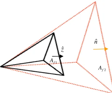
Figure 1 - Definition of the Dual Grid. ... 25

Figure 2 - 2D Unstructured Grid Before Adaption. ... 31

Figure 3 - Adapted 2D Unstructured Grid without Weight Function. ... 31

Figure 4 - Density Contours of Perturbations After Adaption. ... 32

Figure 5 - Adapted Grid with Artificial Sink. ... 33

Figure 6 - Density Contours from Adapted Sink Grid. ... 33

Figure 7 - Definition of Medial Dual Grid. ... 36

Figure 8 - Volume Displacement from Adaption. ... 37

Figure 9 - Motion Vector to Define Face Displacement. ... 41

Figure 10 - Geometry of 2D Dual Grid with Motion Vector. ... 44

Figure 11 - Artificial Sink using New Gridspeed Definition. ... 46

Figure 12 - Adapted Shock Tube Grid. ... 46

Figure 13 - Adapted Solution Compared to Theory. ... 48

Figure 14 - Unadapted Grid Compared to Theory. ... 49

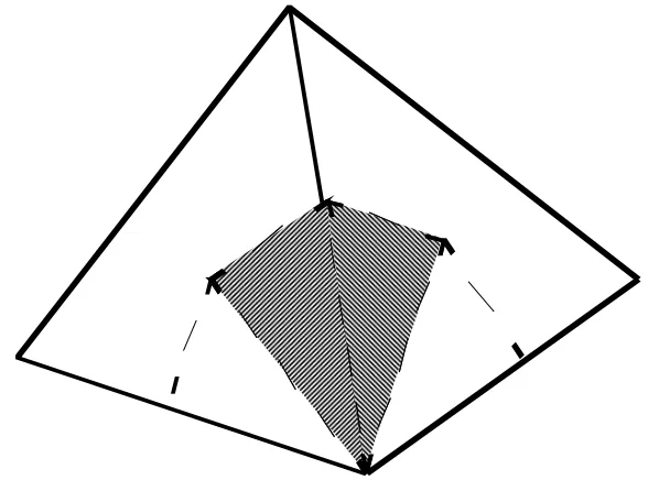
Figure 15 - Adapted 3D Sub-Volume. ... 59

Figure 16 - Volume change from 3D face displacement. ... 60

Figure 17 - Sub-Volume Calculation. ... 61

Figure 18 - Transient Grid Wave Moving in Positive X. ... 67

Figure 19 - Transient Grid Wave Moving in Negative X. ... 68

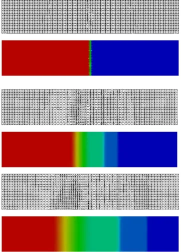
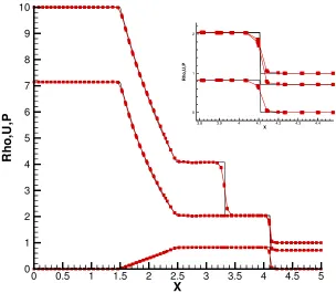
Figure 20 - Shock Tube Results for Starting, Middle, and Intermediate Solution. ... 73

Figure 21 - Unadapted Shock Tube Results. ... 74

Figure 22 - Adapted Shock Tube Results. ... 75

Figure 23 - Airfoil Surface and Volume Resolution. ... 80

Figure 24 - Near Body Resolution. ... 80

Figure 25 - Trailing Edge Resolution. ... 81

Figure 26 - Grid Motion Region. ... 82

Figure 27 - Grid Displacement for Top and Bottom of Cycle. ... 83

Figure 28 - Vertical and Horizontal Plot of Pressure Across Motion Region. ... 86

Figure 29 – PIV Velocity Data (Left) Compared to Laminar Results (Right). ... 87

Figure 30 – CFL3D Laminar Velocity (Left) Compared to Laminar Results (Right). ... 89

Figure 31 – PIV Velocity Data (Left) Compared to Spalart-Allmaras Results (Right). ... 91

Figure 32 – PIV Vorticity Data (Left) Compared to Laminar Vorticity (Right). ... 92

Figure 34 - Comparison of 2D (Left) and 3D (Right) Vorticity Results. ... 94

Figure 33 – Iso-Surface of Vorticity Magnitude. ... 96

Figure 35 - Comparison of 3D (Left) and Delta (3D-2D Right) Vorticity Results. ... 97

Figure 36 - Leading Edge Grid and Spanwise Facetization. ... 98

Figure 37 - Linear Forms of Poor Quality Tetrahedra. ... 110

Figure 38 - Planar Forms of Poor Quality Tetrahedra. ... 111

Figure 40 - Face Swap Example. ... 118

Figure 41 - Canonical Form for 4 and 5 Cell Configurations. ... 119

Figure 42 - Canonical Form for 6 Cell Configurations. ... 119

List of Symbols

a

Speed of Sound

f

A

Face Area

m i A

A±,

Jacobean Matrices

c

Chord Length

e

Internal Energy

E

Split Flux

T

E

Total Energy

h g

f, ,

Inviscid Flux Vectors

p

f

Frequency for Plunging Airfoil

F

Total Flux

H

Total Enthalpy

h

Reduced Plunge Amplitude l/c

j

iˆ, ˆ, ˆ

Direction Unit Normal Vectors

I

Identity Matrix

k

Coefficient of Thermal Conductivity

f

k

Reduced Frequency

l

Physical Plunge Amplitude

M

Mach Number

nˆ

Cell Face Unit Normal

i n N

N ,

Number of Neighbors of a Node and Cell

P

Point or Node Location or Pressure

Solution Vector of Dependent Variables

t s

r, ,

Viscous Flux Vectors

r

rˆ,r

Direction Vectors for Movement or Interpolation

S

Cell Face Area

t

Time

T

Temperature

w v

u, ,

Velocity Components

n

U

Velocity Normal to a Face`

V

Volume

V r

Velocity

f

zˆ

Cell Face Motion Normal Vector

Integration Scheme Coefficient

∆

Difference Operator

ε

Small Number on the Order of Machine Zero

γ

Ratio of Specific Heats

2 1,η

η

First and Second Order Coefficients

Solution Difference Vector

ρ

Density

σ

Weight Function Biasing Coefficient

Implicit Operator

yy xy xx τ τ

τ , ,

Shear Stress Components

Weight Function

Subscripts

f

Face

k

Weight Function Variable, Runge-Kutta Weight

n

Node

m

Neighbor Node or Cell

n

Normal to a Cell Face

Previous Time Level

i

Cell

r

Ratio

s

Sub-iteration

Time Derivative

z y

x, ,

Coordinate Directions

min,

Minimum or Maximum Value

cm

Center of Mass

Superscripts

0

Previous Time Level

C

Convective Flux Components

Newton Sub-iteration Level

n

Time Level

P

Pressure Flux Components

m , , ,−±

Advances in unstructured flow solvers in recent years have enabled engineers to

obtain solutions on increasingly complex geometries, thereby moving unstructured

methods to the forefront of applied computational engineering. Advantages of

unstructured methods lie in the ability to generate grids of reasonable quality around

complex shapes, owing in large part to the lack of implicit ordering and connectivity.

Implicit in this advantage, however, is the need to explicitly define grid connectivity, thus

increasing the overhead of unstructured methods. Control of element count is therefore

desirable to reduce the resource requirements associated with the method for a given

solution, without sacrificing resolution and accuracy. Resolution can be addressed to a

limited degree in the grid generation process by pre-clustering elements in regions of

known interest, such as a body wake. In cases where a priori knowledge of the flowfield

is unavailable, adaption techniques can be used to resolve areas of interest dynamically as

the solution evolves. Adaption techniques can be grouped generally into two types:

enrichment and movement. Enrichment techniques add elements where resolution is

required and potentially remove elements where reduced resolution would not adversely

affect the solution. Aside from the complexity of implementing an enrichment scheme in

a general unstructured solver, enrichment carries the extra burden of increasing the

computational overhead as cells are added. In the case of transient flows, the increase in

cell count can be large if not coupled with a robust coarsening scheme. Movement

increased element count, and add only a modest overhead in computing the grid

movement. Although each method has advantages and disadvantages, movement

methods are generally easier to implement and result in less overhead.

One current shortcoming of both methods, however, is the inability to provide

accurate solutions to transient problems without introducing perturbations into the

solution as the grid is adapted. Development of a conservative, time accurate adaption

method for unstructured grids would expand the scope of solutions obtainable for

transient flows.

In a recent survey of applied CFD methods, Rumsey and Ying1 concluded that

numerical error was often the primary cause of inaccurate lift predictions for high lift

configurations, frequently exceeding modeling error. Venditti and Darmofal2 in their

work on adaption methods noted that the dominant reason for inaccurate predictions of

computational results has been identified as grid resolution. It is agreed generally that

sufficient grid resolution is necessary for the consistent and accurate prediction of flows

and forces on aerodynamic bodies. Unfortunately, grid resolution as viewed from the grid

generation process is analyst dependent, or at least dependent on the principles involved

in the grid generation process. At best it requires a priori information about the flowfield

to develop a grid of sufficient resolution. Resolution thus becomes more of a subjective

and less objective process by which the flowfield is resolved. Adaption has been

developed as a way to mitigate problems associated with resolution of the initial grid by

Unstructured adaption algorithms are often favored over structured grid approaches in

much of the current research because structured grid approaches cannot support the dual

needs of increased geometric complexity and localized resolution without upsetting the

natural ordering of the grid1. Any fully anisotropic adaption scheme for a structured grid

would require explicit ordering, and result in a method comparable in complexity and

overhead to unstructured methods. Unstructured methods, by definition, maintain data

structures to explicitly define grid connectivity which results in substantial overhead but

provides a method to generate a grid for most geometries of interest. These methods also

provide a framework whereby selected areas of the flow can be resolved independently of

the local topology to increase resolution and accuracy through the use of adaption.

The three methods available to adapt unstructured grids are r-refinement (movement),

h-refinement (enrichment), and p-refinement (reconnection)3,4,5. Most of the research in

unstructured grid adaption has focused on enrichment schemes represented primarily by

h-refinement approaches4,5,8,9,10,11,12. H-refinement enrichment schemes use an error

estimator to determine regions of the grid where the solution is under resolved, and add

elements locally to improve the resolution and (hopefully) the accuracy of the solution.

While enrichment schemes have demonstrated the ability to improve solution accuracy

through local refinement4, there is added overhead in the form of increased cell count.

For steady state solutions, the increased overhead is incidental assuming the resolution is

needed to provide the spatial accuracy required for convergence. For transient flows,

enrichment can increase the overhead unnecessarily unless coupled with a robust

Besides the obvious issues of increased overhead, there are more subtle issues of grid

quality that can arise from enrichment. Speares and Berzins13 have developed a time

dependent 3D unstructured adaption algorithm built strictly upon h-refinement. In their

approach, they subdivide selected tetrahedral elements by either edge bisection or

introduction of a new node at the center of the selected tetrahedral. A drawback of this

approach is that the grid quality, where quality in this case is defined only in terms of cell

geometry, will decay over time as a given element is repeatedly subdivided. Without a

smoothing algorithm to recover the grid quality, the number refinement iterations are

artificially restricted, limiting the amount of resolution which can be added to the grid.

Cavallo and Baker4 in the description of their edge splitting technique noted the need to

implement a p-refinement algorithm for edge and face swapping to remove elements

contributing to poor quality. In their approach, a locally constrained Delaunay approach

is implemented which effectively results in local mesh reconstruction to increase

resolution. Local reconstruction usually improves grid quality, but does not prohibit poor

quality.

Grid quality, both for grid generation and adaption algorithms, has proven to be a

difficult subject and one that has been the focus of much research. Freitag and Knupp5

outline nine independent tetrahedral cell configurations which can result in poor quality

cells and affect accuracy. Each of these cell types is a possible result of successive

iterations of enrichment algorithms if applied without mesh smoothing to improve

quality. Structured and 2D unstructured methods have typically used Laplacian

Laplacian smoothers may not only fail to improve poor quality cells, but can degrade

quality, especially in regions of varying connectivity. To improve cell quality, the use of

an optimized mesh smoother based on a quality function is necessary. Frietag and

Ollivier-Gooch6 have developed a best practices approach which incorporates

p-refinement in the form of edge and face swap, with r-p-refinement performed by a

Laplacian and an optimization based smoother to improve grid quality. Application of

these two methods in combination has demonstrated improved mesh quality on grids

where Laplacian based smoothers fail. In this context, however, it should be noted that

quality is measured in purely geometric terms, which may not describe the best structure

to resolve flow gradients, as shown by Laflin14.

Measures of grid quality are typically restricted to a geometric description of quality

based on quantities such as minimum angle or aspect ratio, for example. Viewed in a

broader context, quality is best described in terms of errors produced from the

discretization relative to the underlying solution. McRae and Bond15 have proposed an

alternate view of quality which includes elements of the underlying solution in

determining grid quality. The result is a universal grid quality metric based on an

equidistribution principle that defines quality in terms of cell face alignment with the

local gradient. By aligning the cell face with the local gradient, errors in the flux

calculation are reduced resulting in improved accuracy. In terms of this metric, the

typical aesthetic view of quality, where skewness and stretching are considered to result

high gradient, such as shock waves, actually benefit from skewness if face alignment with

the local Riemann problem is improved.

In order to maintain quality, research has shown that enrichment methods require

either a limited form of adaption or some form of smoothing algorithm to improve grid

quality after enrichment. Restricting adaption presents obvious issues of restricted

resolution and limited improvement in accuracy. Addition of a smoothing algorithm

incorporates r-refinement, and reintroduces the need to properly account for grid

movement in the flux terms to prevent perturbations to the flow16. Therefore, even when

using enrichment to perform adaption there is a need to develop a time accurate adaption

algorithm to solve transient flows accurately.

Adaption algorithms using r-refinement have received little research focus as noted by

Baker3. Zegeling17 presents development of a r-refinement algorithm for finite

differences, but the application was limited to 1D and 2D solutions. Baines et al18,19

demonstrated r-refinement methods for partial differential equations in 2D, and outlined

the steps necessary to implement a time accurate movement scheme through the

development of gridspeed terms and corrected velocities as applied to elliptic problems.

Movement algorithms generally operate through the equidistribution of a weight function.

The weight function, much the same as the error function, is designed to identify areas of

the grid where more resolution is required. Once the weight function is defined, the

weights are distributed throughout the grid resulting in higher resolution in areas

identified by the weight function. Areas where the weight function is small and evenly

clustered to increase resolution in areas where the weight function is large. Determining

an appropriate weight function distribution can be more problematic for 3D unstructured

grids.

Tezduyar20,21 has performed considerable research in the area of moving bodies, such

as a rotating propeller blade, where body surfaces are translated in the grid to simulate

movement. The focus of the approach is to simulate movement rather than to improve

accuracy, but the principles involved are the same in as much as the grid is deformed via

node movement as the body surface is moved, and a method to recover the solution after

movement is required. In this case, interpolation to the new grid was used to transform

the solution from the old grid to the new grid.

Research on methods to maintain accuracy and conservation of the solution during

node movement has primarily centered on structured grids, using either a coupled or

decoupled approach to advance the solution. Decoupled approaches require an

interpolation scheme to update the grid after adaption, and enjoy the advantage of being

independent of the integration scheme and the flow solver in general. A decoupled

approach was developed by Benson and McRae22,23 and expanded by Laflin14 where the

computational domain was utilized to perform movement, and the solution was then

interpolated to the new grid level. The algorithm proved to be very efficient, but use of

the computational domain precluded its use for any unstructured grid approach.

Moreover, the use of interpolation on unstructured grids is more problematic, and

involves the use of computationally expensive algorithms to determine the interpolation

A coupled approach was previously investigated by Klopfer and McRae24 for explicit

solvers and by Orkwis and McRae25 for implicit solvers. Neaves26 successfully

implemented the coupled approach in a 3D implicit structured code to analyze inlet

unstarts. In the coupled approach, the grid is moved using the standard node movement

algorithm, then the flux terms are adjusted to account for the node movement in the

interface velocity. The integration algorithm is modified to account for the resultant

volume change, and, in this case, the time accurate sub-iterations of Rai27 were used to

recover time accuracy at each timestep.

Despite the lack of portability, a coupled approach presents several advantages over

the decoupled approach for unstructured grids. Issues with defining a separate

interpolation method are avoided using the coupled approach, and the robustness of the

integration scheme is utilized to update the solution after each adaption step.

Development of appropriate gridspeed terms can ensure conservation and thereby prevent

additional perturbations to the flow. Once gridspeed terms have been defined,

incorporation of the terms into the flux scheme is straightforward. Modification of the

integration scheme to define an unsteady residual and sub-iterations to recover time

2

Adaption Algorithm

The goal of adaptive grid algorithms is to improve the accuracy of the solution and

reduce analyst dependence through the appropriate resolution of salient features in the

flowfield. Most adaption methods incorporate an error estimator to determine areas of

the solution where there are large values of the error function as defined by the integration

method. Determination of solution error is an ongoing field of research, but a common

approach is to approximate the error through the use of solution gradients. All numerical

approximations to governing equations result in some form of truncation error consisting

of solution derivatives multiplied by powers of the local grid spacing. Truncation error

can be used to estimate errors in the solution and identify regions of the flowfield that

require additional resolution. The goal of additional resolution by any means is to reduce

the local spacing and thereby reduce the local truncation error.

Several methods are available to estimate the location truncation error. A precise

approach would be to determine the exact form of the truncation error terms based on the

numerical method used in the flow solver. Although the first truncation error term is

generally sufficient to approximate the error, a more precise determination of the error

term would require determination of many truncation error terms, which must then be

approximated and evaluated locally to determine the local error. A drawback of this

approach is that it cannot be generalized as the truncation error is unique to each

numerical method and is thus restricted to the flow solver for which the error terms are

solution gradients formed from first order gradients in the flowfield. First order gradients

can be used to approximate higher order solution derivatives by taking the differences of

the first order terms, which vary at a rate proportional to the higher order terms28.

Increased computational efficiency and reduced round-off can be accomplished through

the use of undivided differences in the error estimator, and normalized by the local

values. Normalized undivided solution differences form the basis of the error estimator

used in the current work.

Once an error estimator is defined and implemented, a method to reduce the local

spacing based on the local error function is needed. Two general approaches to this

problem are enrichment and movement. As noted earlier, the typical approach is to use

enrichment to locally refine the grid where the solution error is large, however there are

many complications associated with enrichment algorithms that make their

implementation difficult for unstructured grids. One of the biggest obstacles is the local

data structure of the flow solver. Unlike structured grid methods, which generally employ

an explicit i,j,k ordering scheme, unstructured solvers must explicitly define connectivity

between each node and each cell in the grid. Unstructured grid generators and flow

solvers employ a number of different techniques to construct the grid and compute the

solution. For example, grid generators can use a hyperbolic advancing front technique, or

a top down octree type approach. Flow solvers can be cell centered, or vertex based with

a dual grid that can be defined a number of different ways, such as a median dual.

Differences in the grid generation and flow solver approaches results in a number of

each approach. An enrichment scheme can be developed for each of these methods, but

generalization is difficult and will require modification of the local data structure at some

level.

In addition to issues with the local data structure, parallelization can pose a number of

problems in the context of enrichment schemes. Implementation issues arise at

inter-zonal processor boundaries that are dependent on the enrichment scheme being employed.

Face splitting schemes can be the easiest to implement since the face split is independent

of information on each processor. Edge splitting is difficult because the order of

operations determines the resulting face geometry if the edges of a face are split more

than once during a cycle. Care must be taken to ensure the order of operation at the

inter-zonal boundary is consistent for each processor so that the same adapted grid structure is

produced on each processor. In addition to cell splitting issues, smoothing algorithms can

become complicated at the inter-zonal boundary. Laplacian and optimized smoothing

algorithms are node based methods which can be implemented with an acceptable amount

of overhead at an inter-zonal boundary. Edge swap techniques, however, become

increasingly complex at an inter-zonal boundary since they necessitate a new local

definition of the inter-zonal connections between processors, due to changes in the local

grid structured as a result of the swap.

An important limitation of enrichment schemes is the added computational overhead

incurred, especially for parallel implementations. Enrichment schemes by nature add

cells to the grid structure to provide increased resolution of the flowfield. In a parallel

resolved as a result of the adaption process, leading to an increased load on processors

where there are concentrations of enrichment, and leaving other processors idle while the

adaption cycle completes. If left unchecked, this can lead to a severe load imbalance and

requires rebalancing of the parallel problem. Some parallel distribution codes such as

ParMETIS29 contain routines designed to provide a new distribution to rebalance the

problem after enrichment, but rebalancing can require a substantial cost in

communications overhead, and thus increased solution time. For flows with transient

features, the need to adapt frequently can make enrichment schemes prohibitively

expensive and can require a robust coarsening scheme to prevent the cell count from

becoming unmanageable.

Node movement schemes, by contrast, can be generalized to accommodate multiple

flow solver variants and formed independent of the grid distribution across multiple

processors. Since no cells are added or removed from the domain, the parallel problem

never becomes unbalanced and there is no need to redistribute the grid as the adapted

solution evolves. Construction of a local mesh, including a node and its surrounding

cells, allows generalization of the node movement algorithm independent of the

underlying flow solver. The result of the node movement scheme is a new node location

based on the movement algorithm, which is updated independent of the flow solver and

does not require alteration of the underlying data structures. Some modifications are

most likely required to produce a local grid structure for a node, but these modifications

are in addition to the data structure native to the flow solver and do not require alteration

movement is dependent only on the local data structure of the movement algorithm,

which is true for inter-zonal nodes as well as nodes that lie within the grid domain of each

processor. The ability to define a generalized approach with low computational overhead

make movement schemes an attractive alternative to enrichment schemes for adaption

based algorithms. Therefore the current research is focused on an unstructured node

movement scheme which is both robust and preserves time accuracy.

2.1

Unstructured r-Refinement Adaption

Development of the current unstructured adaption algorithm is based on the structured

grid adaptive algorithm originally developed by Benson and McRae22,23,30,31,32. Extension

of the Benson and McRae method to unstructured grids required modification of the

original method for use in a generalized unstructured approach33. Specifically, the

original method applied grid motion to the computational domain, which was then

mapped onto to the physical domain. Solution variables from one grid level to the next

were interpolated based on the previous grid and solution applied to the new grid after

adaption. Since no computational space exists for an unstructured grid, the method is

modified to perform movement in physical space. In place of an interpolation scheme,

grid motion was coupled to the flow solver via gridspeed terms developed from the grid

motion. Coupling the grid motion to the flow solver allowed for development of an

adaption scheme which was both conservative and maintained the accuracy of the original

Most concepts of the original adaption algorithm, however, are maintained in the

current approach. As with the original method, node movement is based on a center of

mass calculation using a weight function developed from solution differences. Weight

function construction is based on solution differences by means of user supplied biasing

coefficient that select flow variables of interest to form the solution weights. Solution

differences are combined to form the weight function used to perform the center of mass

calculation, where the weight function is analogous to the monitor surfaces described by

Eiseman34. Changes are required to the original weight function and center of mass

definitions to account for the non uniform connectivity associated with unstructured

grids. Clipping operations described with the original method33 are maintained to provide

an even distribution of resolution to strong and weak features in the flowfield. A weight

function spreading operation is performed to determine how far a point is moved in each

adaption cycle. The result is a generalized movement algorithm which can be applied to

unstructured grids in two and three dimensions.

Application to three dimensional grids revealed limitations of the original 2D method

which must be addressed. The Laplacian operator used to perform the center of mass

calculations acted as a natural smoother for structured and two dimensional unstructured

grids. When applied to three dimensional grids, however, the Laplacian operator is

unable to detect many of the grid quality deficiencies, such as spikes, slivers, and spires,

associated with tetrahedral meshes and is therefore unable to provide adequate smoothing

in these regions and in many instances will invert cells if care is not taken. Motion

such as spikes and slivers are difficult to detect with an elliptical smoother, and there is as

yet no common approach which will identify and properly handle all of the geometrically

poor cell types6. Extension to three dimensions therefore necessitated the addition of an

optimization based smoother that can address all types of grid deficiencies in the

tetrahedral mesh, providing improved cell quality without inverting the grid. Details of

the smoother are included in Appendix A.

The following sections describe details of the new adaptive grid algorithm with the

modifications necessary for application to unstructured grids. Details of the weight

function are developed first, followed by development of the center of mass routine.

Node movement restriction routines are described in later sections pertaining to

implementation in two and three dimensions, since different techniques were required for

each application.

2.2

Weight Function

Formation of the weight function is based on solution differences which are used to

approximate solution error for each cell. In this instance, differences are the absolute

undivided differences of the flow quantities stored at each cell. Two dimensional

solutions for the current work are based on a cell vertex description of the flowfield,

meaning that the flow quantities are stored at the node locations. Difference equations

are formed by differences between a node and all the associated neighbor nodes based on

break the weight into component directions. The resulting difference equation is expressed as ) ( ˆ , 1 ) , ( , , ) , ( , , ε φ + − =

∑

where rˆ_(x,y) represents a unit direction vector connecting the nodes, Q represents the

flow quantity of interest for the difference operator,Nn is the number of neighbors

associated with each node, andε is a small quantity to prevent divide by zero. The local

quantity of interest is included in the denominator to prevent overweighting of flow

quantities in regions where very large flow gradients are present35. Inclusion of the

neighbor node count in equation 1 is necessary to ensure that the weight function is not

biased by the local grid connectivity. Unlike structured grids, unstructured grids do not

contain uniform connectivity. Therefore the summation of difference terms must be

normalized to remove the influence of changes in grid topology that are not related to

actual solution differences. Division by the count of neighbor nodes will thereby reduce

biasing due to grid topology. Currently, undivided differences of density, pressure, Mach

number, and velocity components are used to form the weight function.

For three dimensional calculations, a different flow solver was used that required

storage of the solution variables at the cell centers instead of the cell vertices. In the three

defined by the local cell face connectivity, giving a new form of the difference equation as ) ( ˆ , 1 ) , , ( , , ) , , ( , , ε φ + − =

∑

where rˆ_(x,y) now represents a unit direction vector connecting two cells through a

common face, and N_i is the number of cell neighbors associated with cell. Using cell

differences implies that solution variations are measured only through connecting cell

faces, and not through connecting nodes, potentially reducing the topology used for

constructing the difference equation. Use of node based differences, however, would

require averaging cell data to each of the nodes associated with a cell, and would contain

no more information than is contained in the cell centered definition of the grid. Basing

differences on the cell center data is more consistent with the definition of flow quantities

in the grid, and how the governing equations are solved for a given topology.

After the solution differences are formed, the initial raw weight function is formed

from a linear combination of the difference equations for each coordinate direction,

representing a maximal collapse in dimensionality36. Weights for each solution

difference equation are included through a user specified biasing coefficient. Biasing

coefficients select which flow quantities are used to define the unified weight function,

where the relative weight of each coefficient determines how strongly each flow variable

coefficients to resolve features of interest. The raw form of the weight function for two

and three dimensional flows is thus defined as

∑

=

=

Nv

k

z y x k z y x k z

y x

1

) , , ( , ) , , ( , )

, ,

( σ φ

ω (3)

where the z component is zero for two dimensional solutions. σ_krepresents the user

defined biasing coefficient used to select solution differences of interest.

The raw formulation of the weight function does not generally provide balanced

resolution of all flow features in a given solution. Features such as shock waves have

very strong gradients, while features such as expansion waves have smaller cell to cell

gradients. Gradients in the vicinity of shock waves vary according to the local shock

strength, which can vary greatly throughout the domain33. Variations in solution

gradients require that a means to balance the weight function is needed if all features of

the flow solution are to be resolved evenly. Although this approach does not minimize

the error function defined from the solution gradients, it will tend to increase the accuracy

of all selected features of the flow solution, weak and strong, not just the strongest

features. Implicit in this assumption is the fact that the truncation error is not the only

determining factor in solution accuracy.

A clipping operation is performed on the raw weight function to enforce a balance

between strong and weak features in the flow. The purpose of the clipping operation is to

reduce the relative weight of stronger features in the flowfield, while increasing the

relative weight of weaker features. Two user specified input parameters are defined to

weight function values can vary from one solution to another, the maximum and

minimum values are specified as percentages of selected global measures of the current

solution. Percentages are applied to the global range of the current weight function, with

any values above the maximum percentage or below the minimum percentage eliminated.

Clipping the weight function can also eliminate some of the numerical noise associated

with the solution, and thereby focus the adaption on significant solution differences. Care

must be taken in selection of the percentages to not over damp the raw weight function.

Specifying a maximum that is too low will tend to eliminate adaption to any strong flow

features, while a high minimum value will treat weak features the same as regions with a

zero gradient. The equation for the clipping function is given as

) ),

,

min(max( _{( , , ) min,( , ,) max,( , , )} )

, ,

(xyz ω xyz ω xyz ω xyz

ω = (4)

where the min and max values are defined from the user defined percentages applied to

the global weight function.

The resulting weight function contains discontinuous first derivatives throughout the

flowfield as a result of the clipping operation. These discontinuities are eliminated by

applying a Laplacian smoothing operator to the weight function. Smoothing also blends

the weight function so the grid motion is not localized to a feature, such as a shock wave,

resulting in a discontinuous change in the volume ratio between cells. Smoothing leads

to increased resolution of the feature over a wider region of the flowfield and provides

better blending to the unresolved portions of the flowfield. To ensure resolution of the

original values in the method defined by Laflin14, resulting in the following form of the

smoothing operator in two dimensions

n N m y x m y x n y x n N n + + =

∑

with the three dimensional form given by

i N m z y x m z y x i z y x i N i + + =

∑

where summation occurs between a node and all neighbor nodes for two dimensional

solutions, and between a cell and all neighbor cells for three dimensional solutions.

After formation, the individual solution weights are clipped for balanced resolution,

smoothed and then combined in a linear fashion to form a unified weight function. This

scalar function is applied equally to each coordinate direction. While it is possible to

generate a weight function for each coordinate direction for a structured grid approach,

which can then be applied sequentially to promoted alignment of the structured grid with

strong features during the adaption process, the lack of preferred direction in an

unstructured grid makes this process inappropriate. Local grid adaption for unstructured

grids depends on the local grid connectivity, so no a priori prediction of a preferred

direction for the grid adaption can be made.

The last operation applied to the solution weights is a rescaling function. Grid motion

for the current algorithm is determined by a center of mass calculation described in a

central node based on the local weight function values. Overweighting one region of the

grid forces the node closer to the higher weighted regions of the grid while moving away

from regions with lower weights. Implicit in this calculation is that the displacement

distance experienced by each node will be a function of the weight distribution. Regions

with larger local variation of the weight function will experience more relative motion

compared to regions where the weights are nearly uniform. Rescaling the weight function

can take advantage of the center of mass calculation by changing the distribution of the

weight function to control how far a cell is displaced during each adaption cycle.

Ramping of the scale can add further robustness to the calculations by allowing the user

to control the amount of motion performed by the adapter as the solution develops. High

initial perturbations at solution startup can be damped by scaling down the weight

distribution initially, and ramping up to an increased distribution as the solution evolves.

The rescaling operation is defined as

1 ) 1 ( ) ( ) ( ) , , ( max, ) , , ( min, ) , , ( max, ) , , ( min, ) , , ( + − − −

= xyz

z y x z y x z y x z y x ω ω ω ω ω ω (7)

where here the min and max values represent the range of weight function values defined

by the rescaling operation, and the new range is defined as from 1 to the maximum

current value specified by the user. Equation 7 represents the final form of the weight

2.3

Node Movement and Restriction

Node movement is accomplished via a center of mass calculation analogous to the

form used for structured grids. For structured grids, node movement is performed for

each coordinate direction independently in computational space. Unstructured node

movement uses a unified, rescaled weight function defined in the previous section in the

center of mass calculation applied to physical space. New node locations are determined

by the sum of the product of the weight function with the coordinate locations for each

node and connecting node in two dimensions, and by each cell attached to a node in three

dimensions. In each case, the sum is normalized by the total weight function value of a

node and all neighbors. In two dimensions, the center of mass calculation is expressed as

∑

∑

and the three dimensional form is given by

∑

∑

where in the two dimensional case the summation is performed over a node and all the

connecting nodes, while the summation occurs over all of the cells incident on the node in

the three dimensional case. In the three dimensional case, weight values are assigned to

the cell centers and not to the nodes. Therefore the center of mass calculation relocates

current node. Additionally, since the weights are located at cell centers, a natural form of

motion restriction is implemented since the volume defined by the center of mass routine

is restricted to the region defined by the cell centers and not by the node locations.

Barring large distortions in the grid, such as sharp corners, application of the center of

mass calculation should not generate grid crossover. In practice, unfortunately, regions of

poor grid quality produce localized geometry that is similar in structure to sharp corners

or other types of problematic geometry. Issues related to poor grid quality and crossover

3

Unstructured r-Refinement in Two Dimensions

Initial development of the time accurate adaption scheme focused on two dimensional

flows using an explicit two dimensional flow solver for the Euler equations developed as

part of the current research. Development of the two dimensional flow solver begins with

the integral form of the Euler equations given by

∫∫

∫∫

t ) ˆ 0

ˆ ˆ ( (10) where             = T v u P Q             + + = ) ( 2 P e u uv P u u f ρ ρ ρ ρ             + + = ) ( 2 P e v P v uv v g ρ ρ ρ ρ

Integration of the flow solution is accomplished via a four stage Runge-Kutta method

defined as

) ( ~

1 _1,

0 1 ,

1 n k

net k n k n Q F V t Q

Q + + = − ∆ +

α (11)

where F~net(Qn 1,k) +

represents the net flux evaluated at the kth stage of the Runge-Kutta

step, and V represents the volume of the cell. The coefficient α is defined by the

variables are stored at cell vertex locations, and an edge based implementation is used to

perform flux calculations and solution integration. In the cell volume context, this

implementation requires definition of a new volume cell based on the local grid

construction, called the dual grid37. Several options are available for the definition of the

dual grid, and the current implementation uses a median dual grid where cell faces are

formed from endpoints defined by the edge center between two nodes, and the cell center

(area center in two dimensions) of the associated cell. The median dual results in two

faces associated with each grid edge defined by the original grid connectivity, one face

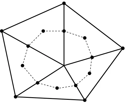
connecting to each cell center to the left and right of the edge as shown in Figure 1.

--Figure 1 - Definition of the Dual Grid.

The solution is advanced in time to a steady state for steady state solutions, or to a

specified time or iteration count for time accurate solutions. In the initial solver, grid

motion was not accounted for in the solution evolution, and grid motion resulted in a

perturbation to the solution. Perturbations from grid motion are iterated out over time for

steady calculations, but these perturbations prevented accurate prediction of unsteady

flows. Extension to time accurate simulations required modification of cell face fluxes to

account for the motion of the grid. Flux calculations at the cell interface are updated to

account for the convective velocity relative to the cell face motion and the integration

scheme is updated to account for the unsteady residual resulting from the volume change

in each cell as the grid moves. The following sections outline the changes to the base two

dimensional flow solver required to produce time accurate predictions for transient flows.

3.1

Modified Integration Scheme

Adaption of two dimensional grids results in volume changes in each cell which must

be accounted for in the integration of the conservation law. The volume is usually

constant for the integral of equation 10, resulting in the form shown in equation 11.

When taken in the context of grid adaption the cell volume is no longer constant and must

be retained as such in the time integration. The result is a non-linear term consisting of

the volume multiplied by the solution vector represented as

) ( ~ )

( 1

1 1

+ +

+

− = ∆

− n

net n

n n n

Q F t

Q V Q V

(12)

Linearization is achieved by expanding the equation at the new time level and

defining an unsteady residual term which incorporates the variation of volume and the

solution as the equations are evolved in time. The resulting unsteady residual is solved

by incorporating sub-iterations to remove the effect of volume change as the solution

) ( ~ , 0 , , 1 1 k n net n n k n n

unsteady F Q

t Q V Q V R + ∆ − = + + (13)

which must be driven to zero to maintain time accuracy. The sub-iterations are

performed using the four stage Runge-Kutta method applied to the unsteady residual. The

modified Runge-Kutta33,38 is defined as

unsteady n n k n R V t Q

Q +1, +1 = ₀ − 1 ∆₊₁

α (14)

where the flux value in equation 11 is replaced by the unsteady residual defined in

equation 13. A new sub-iteration time step has also been introduced. The new timestep is

a pseudo timestep introduced to perform sub-iterations to advance the solution from time

level n to time level n+1. The sub-iteration timestep is defined as

s s i t CFL t t ∆ + ∆ = ∆ 1 1 1 (15)

where CFLsrepresents the CFL value for the sub-iterations and ∆ti represents the pseudo

timestep for the sub-iterations. Converging the sub-iterations to a specified tolerance at

each time step regains the time accuracy after the grid movement.

3.2

Flux Corrections

The flowfields under consideration are governed by the unsteady two dimensional

Euler equations. The equations are modified to include the grid movement terms resulting

equations represent the governing equations for unsteady inviscid flow with grid

movement.

In the context finite volume solvers, the result of the above modification is an

adjustment to the inviscid interface flux to account for the cell face movement. The

modification of the cell face flux is easily made to any upwinding scheme which splits the

inviscid interface flux into convective and pressure contributions, such as AUSM39,

AUSMV40, and LDFSS41. For example consider the flux defined by

P f c f P c E P A E n V A E E

E= + = ρ _int ⋅ˆ~ + ~ (16)

where the flux is split in convective and pressure contributions. A_f represents the area of

the face and V_int is the convective velocity defined at the cell face based on the cell face

outward normal nˆ. The convective and pressure terms are defined as

            =             = 0 0 1 0 ~ ; 1 ~ P E H v u

Ec ρ P (17)

The convective velocity at the cell face must be adjusted to account for the movement

of the cell face after each adaption step. The first attempt to correct the cell face velocity

used the method developed for structured grids. First the cell face velocity is calculated

using a first order difference equation given by

for the x and y coordinate directions respectively. Values of x_tand y_t represent the

velocity of the cell face in the x and y coordinate directions respectively, while x_f and

f

y represent the locations of the cell face midpoint at the n and n+1 timesteps. These

differences are calculated using the cell face centers of the median dual grid, instead of

the coordinate locations. This was found to give a more accurate representation of the

cell face movement for an unstructured grid. Modifying the cell face convective velocity

to account for the grid movement results in the cell interface flux velocity

(

)

(

)

f u x n A v y n A

A n

V_int ⋅ ˆ = − + − (20)

where nˆ =n_xiˆ+n_yˆj.

Using the interface velocity defined by equation 20 introduces an error in the energy

equation arising from the convection of enthalpy term in equation 17, where enthalpy is a

combination of energy and pressure defined as

(

)

ρ

P E

H T +

= (21)

The modified convective velocity produces a non-physical reduction in enthalpy due

to the pressure term in the convection of enthalpy equation in the flux calculation. A

modification to the enthalpy term in the flux calculation is needed to remove the pressure

correction26 by subtracting

(

)

f xn yn

PA + (22)

This single point definition of cell face velocity has been shown to give temporally

undergo pure translation during adaption. However, for unstructured grids, and

structured grids for more general problems, the cell faces will translate, rotate, and stretch

as a result of node movement. In this case, assuming pure translation of the cell face will

not give an accurate calculation of the cell volume change or the cell face flux. Therefore

a new gridspeed definition is needed which will account for all modes of motion.

3.3

Deficiencies in Gridspeed Definition

To illustrate the conservation problems observed using the previous method, a closed

volume with quiescent initial conditions will be examined. The domain is the same

domain used for the shock tube problems with the pressure ratio set to 1:1. When the 1:1

shock tube is started, there should be no perturbation of the quiescent conditions and all

state variables should remain constant. Using the adaption process in this situation causes

small movements in the grid as nodes are relocated by the center of mass algorithm as the

grid is effectively smoothed. This relaxes the grid to a more uniform distribution of areas.

It also results in small distortions and rotations of the cell faces.

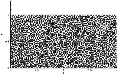
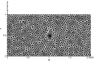
Figure 2 shows the unadapted initial grid. The distribution of cell area in the initial

grid is generally uniform and there are no significant distortions in the cell or node

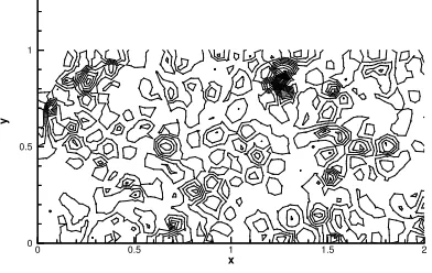
distributions. Figure 3 shows the same section of the domain after five iterations through

the adapter and flow solver, using the initial method of calculating the gridspeed terms

without the averaging process. Since the pressure ratio was 1:1, there are no features

within the flow for the adapter to resolve. To further eliminate any influence from the