ABSTRACT
HUNGERFORD, ASHLEY ELAINE. Three Essays in Spatial Economics. (Under the direction of Barry Goodwin and Sujit Ghosh.)
The first essay examines insurance claims filed with the National Flood Insurance Program. The National Flood Insurance Program (NFIP), a government-run insurance program, has become the largest source of flood insurance in the United States. However, the sustainability of the program has been called into question. The combination of flood insurance rate maps riddled with errors and subsidies to high-risk zones has left the NFIP insolvent. This paper examines alternative methods of premium rating in an attempt to move the NFIP towards solvency. We use single hurdle models to estimate the count of flood insurance claims within the state of Florida. We also model the average indemnity payments for each county. By combining the estimates from the single hurdle models with the estimates for the average indemnity payments, we examine the loss-cost ratios for these counties as well as the expected number of claims. From these results, we can determine the largest problem areas within the state and provide estimates that better reflect flooding risk in Florida.
© Copyright 2014 by Ashley Elaine Hungerford
Three Essays in Spatial Economics
by
Ashley Elaine Hungerford
A dissertation submitted to the Graduate Faculty of North Carolina State University
in partial fulfillment of the requirements for the Degree of
Doctor of Philosophy
Economics
Raleigh, North Carolina 2014
APPROVED BY:
Nicholas Piggott Denis Pelletier
Barry Goodwin
Co-chair of Advisory Committee
Sujit Ghosh
DEDICATION
BIOGRAPHY
Ashley Mabee was born in Santa Maria, California and moved with her family to Bakersfield, California at age 8. She attended California State University, Bakersfield, where she earned a Bachelor of Science degree in Mathematics. At university Ashley met her future husband William Hungerford. Although Bakersfield is renowned for its poor air quality and attempted book bans, Ashley and William left Bakersfield, so Ashley could pursue a PhD in Economics at North Carolina State University. Upon completion of her PhD she will begin employment at Economic Research Services of the United States Department of Agriculture. There she will be reunited with her long-lost office mate, Stephanie Riche.
ACKNOWLEDGEMENTS
TABLE OF CONTENTS
LIST OF TABLES . . . vii
LIST OF FIGURES . . . ix
Chapter 1 Introduction . . . 1
Chapter 2 Modeling of Flood Insurance Claims using Spatially-Varying Zero-Inflated Distributions . . . 4
2.1 Introduction . . . 4
2.2 National Flood Insurance Program . . . 7
2.2.1 History of the National Flood Insurance Program . . . 7
2.2.2 How Flood Insurance Works . . . 8
2.3 Methods . . . 9
2.3.1 Single Hurdle Models . . . 9
2.3.2 Estimating the Expected Number of Claims . . . 13
2.3.3 Modeling Indemnity Payments . . . 14
2.3.4 Implementation . . . 15
2.4 Data . . . 15
2.5 Results . . . 16
2.5.1 Model Estimation . . . 16
2.5.2 Simulating Claims and Indemnity Payments . . . 19
2.5.3 Indemnity Payments . . . 20
2.5.4 Loss Cost Ratio . . . 21
2.6 Discussion . . . 21
2.7 Conclusion . . . 22
2.8 Tables and Figures . . . 24
Chapter 3 Risk Management in Wheat Production . . . 47
3.1 Introduction . . . 47
3.2 Risk Management in Agriculture . . . 48
3.3 Data . . . 51
3.4 Methodology . . . 52
3.4.1 Model for Censored County Yields . . . 52
3.4.2 Prices . . . 55
3.4.3 Risk Management Application . . . 55
3.5 Results . . . 56
3.6 Discussion . . . 60
3.7 Concluding Remarks . . . 61
3.8 Tables and Figures . . . 62
Chapter 4 Spatial Integration of North Carolina Grain Markets . . . 89
4.1 Methodology . . . 91
4.1.1 Mean Modeling . . . 91
4.1.2 Variance Modeling . . . 93
4.1.3 Stochastic Copula Autoregressive Model . . . 94
4.1.4 Comparison to Single Parameter Copulas . . . 96
4.1.5 Non-Linear Impulse Responses . . . 96
4.2 Data . . . 97
4.3 Results . . . 98
4.4 Discussion . . . 102
4.5 Conclusion . . . 103
4.6 Tables and Figures . . . 104
Chapter 5 Conclusion . . . .123
REFERENCES . . . .126
APPENDICES . . . .131
Appendix A Conditional Autoregressive Model (Chapters 1 & 2) . . . 132
Appendix B Prior Distributions for Models (Chapter 1) . . . 133
B.1 Logit Link . . . 133
B.2 Log Link . . . 133
B.3 Modeling Indemnity Payments . . . 134
Appendix C Basics of Copula Modeling (Chapter 3) . . . 135
Appendix D Algorithm for Impulse Responses (Chapter 3) . . . 138
D.1 ObtainingE[Dt+k|t=dt+ν, Dt−1 =dt−1, . . .] . . . 138
D.1.1 Initializing the Shock for an Impulse Response . . . 138
D.1.2 Time Path for Impulse Response After the Shock is Implemented . . 139
LIST OF TABLES
Table 2.1 High risk areas have at least a 1% annual probability of flooding. These areas are referred to as 100-year floodplains. Zones labeled “A” are for inland areas, while zones labeled “V” are reserved for coastal areas. Moderate risk
areas are referred to as 500-year floodplains. . . 24
Table 2.2 Function Forms of the Considered Probability Mass Functions. The function Γ(·) is defined as Γ(n) = (n−1)! and the functionζ(·) is defined asζ(ρ+1) = P∞ k=0 kρ1+1. . . 25
Table 2.3 DIC for Logit Links . . . 30
Table 2.4 DIC for the Log Links . . . 30
Table 2.5 The Chi-Square Statistics for Observations of County-Year Data . . . 30
Table 2.6 The Chi-Squared Statistics for data average over the years for each county. . 31
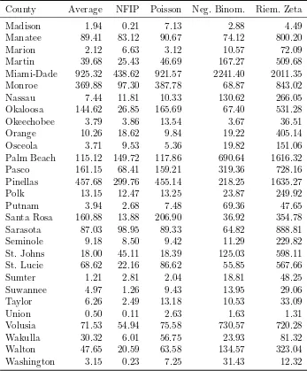
Table 2.7 This table shows the expected losses. The first column is an alphabetical list of all the counties in Florida. The second column is the annual average for historical claims. Third is an approximation of the annual number of claims the NFIP expects. The last three column are show the results for the simulations for each type of hurdle model. For the SHP and SHNB, the simulations for the models with the lowest DIC are shown. . . 32
Table 2.8 DIC for the Indemnity Payment Models . . . 41
Table 2.9 Loss cost ratios . . . 44
Table 2.10 Levee Rating System implemented by the United States Army Corps of Engineers (USACE) . . . 46
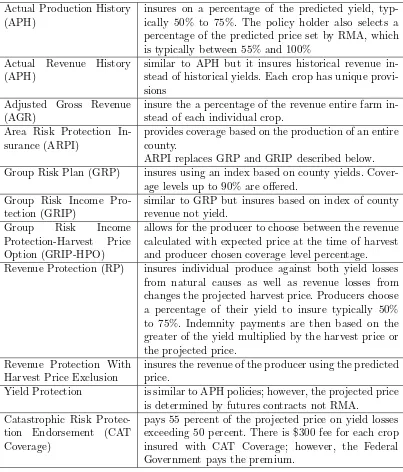
Table 3.1 Descriptions of policies offered by RMA . . . 62
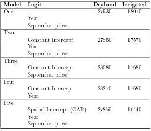
Table 3.2 DIC for the entire model. Here the logit link is varied, while the truncated normal distribution has the spatial intercept, the spatial covariate with the optimal threshold, and the September price. . . 63
Table 3.3 Chi-Squared Discrepancies. “Best-fitting” show the Chi-Square discrepancy of the model that has spatial intercepts with the CAR distribution prior,the optimal threshold covariate in the truncated normal regression, and the September price covariate. “Independent” has different intercepts for each county with independent priors and the September price covariate. These two models have the same logit link. . . 63
Table 4.1 Kendall’s tau coefficient . . . 106
Table 4.2 Results of the Augmented Dickey-Fuller Test conducted on the price series from each terminal grain market. . . 107
Table 4.3 Cointegration Test: Maximal Eigenvalue Likelihood Statistics. An estimate with asterisks ∗ ,∗∗ , or∗∗∗ indicate statistical significance at the α=.10,α= .05 andα=.01, respectively. . . 107
Table 4.4 VAR(1) and GARCH(1,1) estimates and standard errors for the wheat mar-kets. ∆pW G,tand ∆pW S,t are the price different for the wheat markets in
Greenville and Statesville, respectively, on day t. An estimate with aster-isks ∗
,∗∗
, or ∗∗∗
indicate statistical significance at the α =.10,α =.05 and
α=.01, respectively. . . 108
Table 4.5 VAR(1) and GARCH(1,1) estimates and standard errors for the corn mar-kets. ∆pCB,tand ∆pCB,t are the price different for the corn markets in Bar-ber and Laurinburg, respectively, on dayt. An estimate with asterisks ∗ ,∗∗ , or ∗∗∗ indicate statistical significance at the α = .10,α = .05 and α = .01, respectively. . . 108
Table 4.6 VAR(1) and GARCH(1,1) estimates and standard errors for the soybean markets. ∆pSC,tand ∆pSF,t are the price different for the soybean markets in Cofield and Fayetteville, respectively, on dayt. An estimate with asterisks ∗ ,∗∗ , or ∗∗∗ indicate statistical significance at the α = .10,α = .05 and α=.01, respectively. . . 108
Table 4.7 CRPS . . . 109
Table 4.8 Parameter Estimates for the single parameter copulas . . . 109
Table 4.9 Parameter Estimates for SCAR models of Wheat Markets . . . 110
Table 4.10 Parameter Estimates for SCAR models of Corn Markets . . . 110
Table 4.11 Parameter Estimates for SCAR models of Soybean Markets . . . 110
Table 4.12 Half-Lives of Impulse Responses. The half-life is the time (in days) that it takes for the deviation dissipate to half of its distance to the equilibrium. . 122
LIST OF FIGURES
Figure 2.1 Maps Relating to Policies . . . 26 Figure 2.2 Maps Relating to Losses . . . 27 Figure 2.3 The prior and posterior distributions of the covariate of Number of Policies
for the logit link. . . 28 Figure 2.4 For the logit link with the lowest DIC, the 2.5th, 50th, and 97.5th percentiles
of spatial intercepts are shown above. . . 29 Figure 2.5 The prior and posterior distributions of the covariate Number of Policies
for the log link of the SHP model. . . 31 Figure 2.6 For the SHP model with the lowest DIC, the 2.5th, 50th, and 97.5th
per-centiles of random effect intercepts are shown above. . . 34 Figure 2.7 The prior and posterior distributions of τ and the covariate Number of
Policies for the log link of the SHNB model. . . 35 Figure 2.8 For the SHNB model with the lowest DIC, the 2.5th, 50th, and 97.5th
per-centiles of spatial intercepts are shown above. . . 36 Figure 2.9 The prior and posterior distributions of the coefficient for log number of
policies and “Coast” for the SHRZ model. . . 37 Figure 2.10 For the SHRZ model, the 2.5th, 50th, and 97.5th percentiles of spatial
inter-cepts are shown above. . . 38 Figure 2.11 Maps for Expected Losses . . . 39 Figure 2.12 Percentiles for the average indemnity payments (adjusted to 2013 dollars)
for a flood insurance claim. . . 40 Figure 2.13 Percentiles for the simulated average indemnity payments (adjusted to 2013
dollars) for a flood insurance claim. These are based on the model for average indemnity payments, which had the lowest DIC. . . 42 Figure 2.14 Maps of loss cost ratios . . . 43 Figure 3.1 Figures for the entire state of Kansas including the average yield and number
of acres planted. . . 64 Figure 3.2 Wheat price for a per bushel (adjusted to 2013 price) . . . 65 Figure 3.3 Average yield (bushels per acre). Sample period: 1970-2013 . . . 66 Figure 3.4 Prior and posterior distributions of the dryland and irrigated wheat logit
link functions. Note there is noα0 posterior distribution for irrigated wheat
because the intercepts for the best-fit irrigated wheat logit link function are spatially-varying. . . 67 Figure 3.5 Posterior percentiles for the spatial intercepts of the irrigated wheat logit
link. . . 68 Figure 3.6 Prior and posterior distributions for the parameter θ of the dryland wheat
and irrigated wheat . . . 69 Figure 3.7 Posterior percentiles for the spatial intercepts of the dryland wheat
trun-cated normal regression . . . 70 Figure 3.8 Posterior percentiles for the secondary spatial covariate of the dryland wheat
truncated normal regression . . . 71
Figure 3.9 Posterior percentiles for the spatial intercepts of the irrigated wheat
trun-cated normal regression . . . 72
Figure 3.10 Posterior percentiles for the secondary spatial covariate of the irrigated wheat truncated normal regression . . . 73
Figure 3.11 Percentiles for the simulated dryland yields . . . 74
Figure 3.12 Percentiles for the simulated irrigated yields . . . 75
Figure 3.13 Probability for the three coverage levels of dryland wheat of the best fitting model. . . 76
Figure 3.14 Probability for the three coverage levels of dryland wheat of the model with independent counties. . . 77
Figure 3.15 Probability for the three coverage levels of irrigated wheat of the best fitting model. . . 78
Figure 3.16 Probability for the three coverage levels of irrigated wheat of the model with independent counties. . . 79
Figure 3.17 Premium rates for the three coverage levels of dryland wheat of the best fitting model. . . 80
Figure 3.18 Premium Rates for the three coverage levels of dryland wheat of the model with independent counties. . . 81
Figure 3.19 Premium rates for the three coverage levels of irrigated wheat of the best fitting model. . . 82
Figure 3.20 Premium rates for the three coverage levels of irrigated wheat of the model with independent counties. . . 83
Figure 3.21 Distribution of Olympic average of prices . . . 84
Figure 3.22 County probability from the ARC program . . . 85
Figure 3.23 Percentiles of the Olympic averages for dryland wheat. . . 86
Figure 3.24 Percentiles of the Olympic averages for irrigated wheat. . . 87
Figure 3.25 Median of the expected payout for the ARC program. . . 88
Figure 4.1 Acres planted for the three crops of interest . . . 104
Figure 4.2 Daily Market Prices . . . 105
Figure 4.3 Wheat: Gaussian Copula Parameters . . . 111
Figure 4.4 Wheat: Double Clayton Copula Parameters . . . 112
Figure 4.5 Wheat: Double Gumbel Copula Parameters . . . 113
Figure 4.6 Corn: Gaussian Copula Parameters . . . 114
Figure 4.7 Corn: Double Clayton Copula Parameters . . . 115
Chapter 1
Introduction
This dissertation contains three essays that center around spatial relationships. Chapter 2 and Chapter 3 both examine how insurance is affected by the presences of systemic risk. Systemic risk is the probability of losses occurring simultaneously and dependently. If systemic risk is not properly accounted for in insurance ratings, rates may be inefficient and lead to inaccurate probabilities. The third essay, Chapter 4, examines spatial integration of grain markets in North Carolina. If markets are spatially integrated, then the Law of One Price holds. The Law of One Price states that the price of a homogeneous good in different locations is the same when transaction costs are excluded. If the Law of One Price does not hold, this may reflect asymmetric information in the markets.
The first essay examines the National Flood Insurance Program (NFIP). By 2013 the NFIP had accumulated approximately $20 billion in debt, including the losses from Hurricane Kat-rina and Hurricane Sandy, but NFIP collects at most $3.8 billion in premiums per year. Unlike automobile insurance claims or homeowner insurance claims, the correlation among flood in-surance claims is very high. Also some models used for rating flood inin-surance policies, Flood Insurance Rate Maps, are notoriously erroneous. Therefore, we propose a new method for mod-eling flood insurance policies that incorporates the spatial autocorrelation among losses as well as the potential for catastrophic losses as seen during hurricanes.
For our estimation of losses from floods, we use a two part model. The first part of the model estimates the annual count of flood insurance claims in a particular county, and the second
part of the model estimates the average indemnity payment in that county. There are three variations of the model, in which the count part of the model uses different distributions: the Poisson distribution, the Negative Binomial distribution, and the Riemann-Zeta distribution. Both parts of the model account for spatial autocorrelation. This analysis is conducted using data from the 67 counties of Florida during the sample period 1978-2011. The state of Florida is chosen because approximately 40% of flood insurance policies held are for properties located in Florida. After estimating our models, we compare the loss cost ratios derived from the three variations of our model to the observed loss cost ratios of the NFIP.
There has been increasing interest in agricultural risk management, which is reflected in the 2014 Farm Bill; therefore, for the second essay, we turn our attention to crop insurance and the Agricultural Risk Coverage (ARC) program. In this essay, we model yields and prices to determine crop insurance premium ratings and expected payouts from the ARC program. Like flood insurance, crop insurance is susceptible to systemic risk. Natural disasters, such as the drought that struck the Midwest in 2012, cause lower yields for producers over an expansive area. Hence spatial autocorrelation is accounted for in our models of yields. We also expect the spatial autocorrelation to change depending on the quantity of the yield since spatial autocorrelation of yields is expected to be higher during a natural disaster compared to a “good” year. Therefore, we allow for spatial dependency to change based on the quantity yielded.
As mentioned earlier, if markets are not integrated, this could indicate asymmetric informa-tion among markets. Asymmetric informainforma-tion can negatively impact decisions made by market players. The seminal work on market integration kept transaction costs fixed or assumed trans-action costs so high that markets would be isolated. More recent work used regime switching regression models along with impulse response functions that better incorporated transaction costs. Our analysis utilizes non-linear impulse response functions; however, we opt for copula modeling instead of the conventional threshold modeling.
The model estimation in Chapter 4 utilizes weekly price observations from six grain markets in North Carolina. The weekly price series cover a sample period from January 7, 2000 to November 3, 2011 for the two corn markets and two soybean markets, and the sample period for the two wheat markets is from October 7, 2005 to May 27, 2010. The estimation is pairwise, such that the spatial integration is only tested for the same crop markets. After implementing an ARMA-GARCH model on log returns of the prices for each market, we use copula models on the standardized residuals. Therefore, the residuals of the ARMA-GARCH estimations for series of log returns can be correlated, and that correlation is described by a time-varying copula model referred to as a Stochastic Copula Autoregressive (SCAR) model. By using SCAR models in place of regime switching regression to develop impulse responses, changes from equilibrium to disequilibrium and visa-versa are continuous.
Chapter 2
Modeling of Flood Insurance Claims
using Spatially-Varying
Zero-Inflated Distributions
2.1
Introduction
in slightly over $3.8 billion in premiums in 2013. Under the current structure of the NFIP, paying off this amount of debt is impossible. Most of this debt stems from indemnity payments after Hurricane Katrina in Louisana, which amounted to $13.2 billion. The debt accrued from Hurricane Sandy has not been completely realized; however, the federal government did increase the debt ceiling of the NFIP from approximately$20.7 billion to$30.4 billion(GAO, 2013). The current model of the NFIP has grave flaws which allow for these large debts to accumulate. One of the major flaws is the current policy rating system. Therefore, we examine an alternative method of rating that would yield actuarially-fair premiums.
Skees and Barnett (1999) outlined several ideal conditions for insurance including 1) infor-mation between the insurer and insuree should be symmetric, 2) claims should be independent and random, and 3) losses can easily be measured. Flood insurance claims are spatially cor-related due to the systemic nature of flooding. Hence, flood insurance suffers from a lack of independence among claims and systemic risk. Systemic risk is the probability of a large num-ber of losses occurring simultaneously and dependently. Therefore, the second condition listed above is violated. In other insurance markets, such as automobile and fire insurance, loss events are almost completely independent from each other. On the other end of the spectrum, deriva-tives, such as futures contracts and options for a given commodity, are highly correlated. Flood insurance and crop insurance fall in between these two extremes.
The analysis of flood insurance claims and indemnity payments is surprisingly sparse. How-ever, after Hurricane Katrina and more recently Hurricane Sandy, the literature for the supply-side of flood insurance has grown. A series of papers by Kousky and Michel-Kerjan (2009a and 2009b) explore the tail dependence between flood insurance indemnity payments and home-owners insurance indemnity payments from wind damage. Using copula modeling, the authors identify dependence between large volumes of flood insurance indemnity payments and large volumes of wind damage indemnity payments. Similar results were found by Diers et al. (2012) and Pfiefer et al. (2012) for flood insurance indemnity payments and wind insurance indemnity payments in Germany. However, Kousky and Michel-Kerjan (2009a) discarded the observations equal to zero, while Diers et al. (2012) and Pfierfer et al. (2012) aggregated the data, so the
data contained no observations equal to zero. Discarding zeros makes the model conditional on the occurrence of positive observations. Although a conditional model does provide insight, the conditional model cannot be used to rating insurance policies. Also the aggregation performed by Pfiefer et al (2012) is across all of Germany, which would only allow for the calculation of the premium rate for the entire country. Using a model that omits zero values may overstate risk.
2.2
National Flood Insurance Program
2.2.1 History of the National Flood Insurance Program
Before the National Flood Insurance Program (NFIP), flood victims typically had two sources of relief, charities and government disaster relief. Most floods do not warrant government disaster relief, and charities do not offer a stable means of assistance (Federal Emergency Management Agency, 2002). To move the burden of flood disaster relief from taxpayers to floodplain residents and provide a steady means of assistance to flood victims, in the 1950s, Congress attempted to encourage private insurers to provide flood insurance with the Federal Flood Insurance Act of 1956. However, the private sector was not interested in providing flood insurance. After the devastation of Hurricane Betsy in 1965 along the coast of Louisiana and southeastern Florida, Congress stepped forward and passed the National Flood Insurance Act of 1968 (Michel-Kerjan, 2010). From this act, the National Flood Insurance Program (NFIP) was established to provide a government-run flood insurance program to the inhabitants of floodplains.
The NFIP has grown substantially over the last six decades and undergone major reform. Af-ter Tropical Storm Agnes in 1972, Congress passed the Flood Insurance Protection Act of 1973, which required the designation of flood prone areas called Special Flood Hazard Areas (SFHA) and the creation of Flood Insurance Rate Maps (FIRMs). Individuals with federally-backed mortgages for properties located on floodplains are now required to purchase flood insurance. In 1983 the Write Your Own (WYO) program was developed. This program allowed private insurance companies to become intermediaries for the NFIP and sell flood insurance without bearing any risk. Private insurance companies participating in the WYO program receive ap-proximately 30% of the flood insurance premiums. The vast majority of NFIP policies are now purchased through the WYO program. After the devastation of the Midwest Floods of 1993, the National Flood Reform Act of 1994 established initiatives to increase market penetration as well as establishing the Community Rating System (CRS). Communities that enlist in CRS and take preventative measures against floods are able to receive reduced premiums. According to FEMA, the reduction in premiums can be as much as 45% (FEMA, 2013).
For most of the program’s history, the National Flood Insurance Program has offered direct subsidies to approximately 20% of flood insurance policyholders. If flood insurance rate maps were updated and resulted in higher premiums, policyholders with continuous coverage were allowed to “grandfather” their previous insurance rates. The Biggert-Waters National Flood Reform Act of 2012 eliminated subsidies that allowed the grandfathering of rates. These subsi-dies were expected to be completely fade out by 2014. However, in March 2014 the Homeowners Flood Insurance Affordability Act was passed which delayed the elimination of subsidies.
The majority of legislation affecting the National Flood Insurance Program has been enacted to increase market penetration of flood insurance. By increasing market penetration the federal government lessens its obligation to supply disaster assistance after major floods. However, with the focus on increasing market penetration through subsidies, the sustainability of the program has been ignored, except for the short-lived reform of the Biggert-Waters National Flood Reform Act of 2012. Therefore, in order for the NFIP to continue, FEMA must evaluate the premiums needed to achieve solvency.
2.2.2 How Flood Insurance Works
2. Unusual and rapid accumulation or runoff of surface waters from any source, 3. Mudflow, or
4. Collapse or subsidence of land along the shore of a lake or similar body of water as a result of erosion or undermining caused by waves or currents of water exceeding anticipated cyclical levels that result in a flood as defined above.”
Damage caused by wind during a flood is not covered by the NFIP. Likewise, flood damage is not covered by the vast majority homeowners insurance. Property owners who live within a 100-year flood plain (Special Flood Hazard Area) - an area with a 1% or greater annual probability of being flooded- are required to purchase flood insurance if their mortgages are federally-insured. Also many lenders require the purchase of flood insurance if a home is located in a 100-year flood plain. Table 1 shows the Flood Insurance Rate Map (FIRM) designations. Areas designated as a Special Flood Hazard Area (SFHA) also have a “base flood elevation”. This elevation is the expected elevation of flood waters with a 1% probability. The property’s FIRM designation, base flood elevation, and characteristics of the property determines the policyholder’s flood insurance premium.
Interestingly, there is a discrepancy between the definition of a flood and how flood insurance policies are rated. By definition flood insurance policies are covered under the event of a levee breaking. However, the condition of levees is not fully accounted for in policy ratings. This disparity was a contributing factor in the destruction caused by Hurricane Katrina. This issue is yet another reason to consider alternative methods of insurance rating. The Methods section below provides alternative models for rating flood insurance policies. Further information on levee ratings and flood insurance policy ratings is provided in the Discussion.
2.3
Methods
2.3.1 Single Hurdle Models
This paper utilizes Bayesian hierarchical models. Banerjee et al. (2004) provides an excellent overview on spatial Bayesian hierarchical models. In particular we use single hurdle modeling,
which accounts for over-dispersion in the data that may appear due to excess zeros in the count data. If we do not account for the over-dispersion, then the estimated standard errors may be too small and resulting into underreporting Type I error rates within a hypothesis testing scenario. Most counties in Florida exhibit a significant proportion of years having zeros flood insurance claims with the average being 40% of observations for a county. For our modeling, we utilize the single hurdle modifications of the Poisson, Negative Binomial, and Riemann Zeta distributions. The Poisson and Negative Binomial distributions are the workhorses of discrete modeling, while the Riemann Zeta distribution is rarely used the risk management literature.1
The random variable of the annual count of flood insurance claims per a county, denoted as Cit, can be represented as
Cit=Bit(1 +Uit) (2.1)
for County i = 1, . . . , N and Year t = 1, . . . , T. Bit is a random variable distributed as
Bernoulli(Pit), andUitis a discrete random variable with the probability mass functionf(u,θit)
taking values u = 0,1,2, . . .. The representation of Cit leads to the following probability mass
function:
P r(Cit=c|Pit,θit) =
1−Pit if c= 0
Pitf(c−1|θit) if c= 1,2, . . .
. (2.2)
Any single hurdle model can be represented by suitably choosing the parameters Pit’s and
θit’s and the function form f(·|θit).The representation 2.2 can be used to recover the Bit’s and
Uit’s based on observingCit’s in the following manner:
and
Uit=
undefined ifBit= 0
Cit−1 ifBit= 1
. (2.4)
As mentioned earlier,Bitfollows a Bernoulli distribution. The probability parameterPit of this
Bernoulli distribution is modeled using a logit link:
logit(Pit) =αi,0+
B
X
j=1
αijzijt, (2.5)
where (zi1t, . . . , ziBt) denotes the vector of covariates for Countyi and Year t.
To help account for spatial variation among the counties, a Conditional Autoregressive (CAR) model is used for the intercepts of the logit link, such that (α0,1, . . . , α0,N)∼CAR(˜µα, τα2).
The CAR is a popular model based on the notion of Markov Random Fields. The mean (or intercept in our model) of one county is dependent or conditional on the means (intercepts) of other counties and is conditioned on “surrounding” counties. ‘Surrounding” can be defined by distance or contiguity. In this model, we choose contiguity over distance since the counties greatly vary in size and shape. A detailed description of the CAR model is provided in the Appendix A.
Exchangeable prior distributions are used for the covariate coefficients, which are allowed to vary with counties as random effects, such that (αi1, . . . , αiB)iid∼N(¯µα,Σα) fori= 1, . . . , N.
All of the prior distributions are chosen to be vague (i.e. with very large prior variance) but not improper, i.e. the densities of the prior distributions integrate to one. For a detailed list of the prior distributions, refer to the Appendix.
Three different discrete distributions are considered in modeling the unobserved random ef-fects Uit: the Poisson distribution, the Negative Binomial, and the Riemann Zeta distribution.
Table 2.2 shows the functional forms for each of these distributions along with their means and variances. Although the Poisson distribution is a commonly used discrete distribution, the Poisson distribution restricts the mean equal to the variance. Insurance applications pertaining
to natural disasters tend to have extremely large variances relative to the mean value. There-fore, the Negative Binomial distribution is also proposed for our application. The additional parameter,r, allows for a greater range of flexibility to model the variance. Finally, when mod-eling continuous distributions with long tails, the Generalized Pareto distribution is a popular choice as seen in Cooley et al. (2008). The Riemann Zeta distribution is considered the discrete analog of the Generalized Pareto distribution. The Riemann Zeta distribution is capable of hav-ing a very long right tail dependhav-ing on the parameter specification, which makes it a probable candidate for modeling catastrophic risk.
The covariates are liked through the mean, as seen in Table 2, of the unobserved random component Uit. Specifically, letting µit = E(Uit|Zit) we use the following log link function for
the Poisson and Negative Binomial distributions:
log(λit) =β0,i+ B
X
j=1
βjzijt, (2.6)
where zTit = (zi1t, . . . , ziBt) denotes the vector of covariates available for County iand Year t.
The intercepts have the prior (β0,1, . . . , β0,N)iid∼CAR(µβ, σ2β) and the coefficients for the
covari-ates have independent normal distributions for their priors. The parameter r in the Negative Binomial distribution is estimated using a gamma distribution for its prior distribution.
For the Riemann Zeta distribution we must solve for the parameter ρit non-linearly to
obtain the mean of the Riemann Zeta distribution which is µit = ζ(ζρ(itρit+1)) −1 forρit>1, where
ζ(ρit) =P ∞ n=1
1
nρit. We again use the log link function for positive count model, such that
B
following link function:
log(ρit) = log(2) + log(1 +exp(β0,i+ B
X
j=1
βjzijt)). (2.8)
This link function will be used in future research. These single hurdle models are referred to as the Single Hurdle Poisson (SHP) model, the Single Hurdle Negative Binomial (SHNB) model, and the Single Hurdle Riemann Zeta (SHRZ) model.
2.3.2 Estimating the Expected Number of Claims
The purpose of these single hurdle models is to determine the actuarially fair premium rates. The actuarially fair premium rate is the expected value of the number claims for each county, which can be written as
E(Ci,2012) =Pi,2012×E(Ci,2012|Ci,2012 >0), (2.9)
where Ci,2012 is the annual number of claims for county i = 1, . . . , N in the year 2012. The
equation above states that the expected number of claims in a county is equal to the probability of at least one flood claim in that county during 2012 times the expected number of claims for the year 2012 conditioned on at least one flood insurance claim being filed. The actuarially fair premiums can be determined by multiple both sides of the equation above by the coverage. For actuarially fair premiums, premiums should be equal to expected payouts.
For simulating the count of flood insurance claims, we use posterior predictive sampling. Posterior predictive sampling differs from sampling in classical statistics. Posterior predictive sampling is a two part process. Since Bayesian methods treat parameters as random variables, the first part of posterior predictive sampling is drawing parameters from the posterior distri-bution. The samples of parameters drawn from the posterior distributions are then used in the sampling distribution to draw random samples of observations. Posterior predictive sampling allows us to take in to account the uncertainty not only in the sampling distribution but the
uncertainty in the parameters as well. After data are simulated from each type of single hurdle model - the Poisson, Negative Binomial, and Riemann Zeta models, the expected number of flood insurance claims for each county are estimated using Monte Carlo integration. Monte Carlo integration is a method of numeric integration based on simulations that is popular in the insurance industry.
2.3.3 Modeling Indemnity Payments
For modeling indemnity payments, we use the entire monthly data set from January 1978 to June 2012. The indemnity payments are normalized to 2012 dollars. Average indemnity payments are modeled as
Miq =
Riq/Ciq if Ciq >0
Not Available if Ciq = 0
, (2.10)
whereCiq is the number of flood claims andRiq is the total of indemnity payments for county
i= 1, . . . , N during month q= 1, . . . , Q.Miq conditioned on Ciq is modeled with the following
equation:
Miq =φilog(1 +Ciq) +δi,0+
B
X
j=1
δijzijq+ǫiq, (2.11)
where zijq are covariates for county i = 1, . . . , N and month q = 1, . . . , Q. The county level
random effects are modeled as
values in each county, which in turn affects the average indemnity claims. For a detailed list of the prior distributions used in this model, refer to the Appendix.
After estimating the model for the average indemnity payments for each county, average indemnity payments are simulated using posterior predictive sampling. Using these simulated payments in conjunction with the simulations of the count of flood insurance claims, we are able to establish loss cost ratios for each county. The parameters (µφ, σ2φ, ρδ, σδ2, µδ,Σδ) are estimated
using MCMC methods, and posterior inference is obtained.
2.3.4 Implementation
To perform the analysis, the open source softwares R and OpenBUGS are employed. All mod-eling is written in R. Using the software package R2OpenBUGS, the Single Hurdle Poisson model and the Single Hurdle Negative Binomial model are exported to OpenBUGS to perform the Bayesian updating using the Adaptive Sampling Rejection algorithm. This algorithm is discussed by O’Hagan et al. (2004). The Single Hurdle Riemann Zeta model is estimated using the Metropolis-Hasting algorithm, which is discussed by Gilks (1996) but this model is not exported to OpenBUGS because the Riemann Zeta function (a portion of the Riemann Zeta distribution) cannot be estimated in OpenBUGS. Therefore, the modeling of the Riemann Zeta distribution is performed completely in R. The modeling of the average indemnity payments is also performed in OpenBUGS.
2.4
Data
Through two Freedom of Information Act (FOIA) requests, data concerning the National Flood Insurance Program are obtained. Although the first data set obtained from the Federal Emer-gency Management AEmer-gency (FEMA) contained monthly totals of indemnity payments and counts of flood insurance claims for every county in the United States from January 1978 to June 2012, the scope of our analysis is limited to Florida. Florida is chosen because approxi-mately 40% of the flood insurance policies (over 2 million policies in 2012) in the United States
are within Florida and approximately 29% of households in Florida have a flood insurance pol-icy. The data are aggregated annually for the models of the count of flood insurance claims, but we analyze the monthly data when modeling the average indemnity payments. Premiums are determined on an annual basis, hence the use annual aggregation for the count model of flood insurance claims. From the second FOIA request, the data for policies in-force, coverage, and premiums for each county in Florida was obtained. The minimum elevation2 of each county, whether the county is coastal3, and the number of policies are used as covariates through the
link functions as well as modeling the average indemnity payments. Note for the “Number of Policies” covariate, a log transformation is used for an easier interpretation of the covariate and numerical stability.
Figure 2.1 and Figure 2.2 show maps relating to flood insurance policies and losses, respec-tively. The coastal counties, especially southern Florida and the panhandle, have experience the highest losses and have the highest amount of policies in-forced. From causal observation there appears to be spatial correlation, which supports our use of spatially-varying intercepts in the link functions. The highest losses are in counties with a higher cost of living, such as Destin in Okaloosa County (located in the panhandle) and Miami in Miami-Dade County on the southeastern coast of Florida.
2.5
Results
2.5.1 Model Estimation
inclusion of the covariates of “Coast” and “Minimum Elevation” do not improve the estimation of the probability of at least one flood claim occurring. Therefore, when simulated the count of claims for each county, the simplest model, containing only the log “Number of Policies” is included. Figure 2.3 shows the prior and posterior distribution of the coefficient on the log “Number of Policies” for the best fitting logit link based on the DIC. One can see that the prior distribution is very flat compared to the posterior distribution. If the log “Number of Policies” covariate a increases by one unit will lead to approximately a .69% increase in odds of a claim being filed according to the median of the posterior distribution. Figure 2.4 shows the 2.5th,50th,97.5th percentiles of the posterior distributions of the spatial intercepts.
The estimates of the spatial intercepts align with previous expectations that the counties most prone to hurricane exposure have higher intercepts. The maps for the 50thand 97.5thpercentiles show the coastal counties in the southern end of the pennisula, including Miami-Dade, Palm Beach, and Monroe, have the highest spatial intercepts. Other hurricane-prone counties, such as Hilsborough and Pinellas, also have high spatial intercepts.
To compare the positive count component of the single hurdle models, the Poisson, Negative Binomial, and Riemann Zeta distribution estimates, we use DIC as well as Chi-Square statistics. DIC is used to compare the distributions to each other as well as which covariates to include. The Chi-Squared statistics are implemented after selecting the best covariates to include as indicated by DIC. Also the Chi-Squared statistics includes the logit portion of the single hurdle models, but the same logit link is used for all three distributions, so the results of the Chi-Squared statistics reflect only the choice of the positive count distributions. Table 2.4 presents the DIC for the log links of the Poisson, Negative Binomial, and Riemann Zeta components of the single hurdle models with different combinations of the covariates. To assess the predictive abilities of these models, we use the omnibus Chi-squared statistics described by Gelman et al. (2004). Table 2.5 shows Chi-Squared statistics calculated using all 2278 county-year observations, such that 67 X i=1 34 X t=1
(ci,t−E(Ci,t|θi,t))2
V ar(Ci,t|θi,t)
, (2.12)
whereci,t is the observed count of flood insurance claims for Countyiduring Yeart.E(Ci,t|θi,t)
and V ar(Ci,t|θi,t) are calculated from the simulated claims described in the next section.
Intu-itively, the Chi-Squared statistic with the lowest value gives the best fitting model.
Insurance applications are mainly concerned with the average of many years. Even if a model does not predict a flood with a 25 year return interval for a given year, the insurance company can recuperate given the flooding event occurs on average every 25 years. Therefore, we also calculate the Chi-Squared statistic over for the average count of flood insurance claims for each county over the sample period, such that
67
X
i=1
( ¯ci−E( ¯Ci|θ))2
V ar( ¯Ci|θ)
. (2.13)
According to DIC, for the Poisson and Negative Binomial models, the log links that only have the log “Number of Policies” as the covariate are the best fitting, while the Riemann Zeta model has the lowest DIC when the log link contains the covariates log “Number of Policies” and “Coast”. According to DIC the best fitting positive count model is the Negative Binomial model and the worst fitting model is the Poisson model. The Chi-Squared statistics using the county-year observations reflect the DIC for the log links. However, looking at the Chi-Squared statistics for the average count of the flood insurance claims for each county tells a different story. Here the Chi-Squared statistics for the Riemann Zeta model is the worst fitting, while the Negative Binomial and Poisson models show much better fits.
number of claims by .0068 given at least one flood claim is filed. Also Figure 2.7 shows that the posterior distribution ofr for the Negative Binomial model is relatively close to zero, which indicates the Negative Binomial model substantially differs from the Poisson model. Recall that r → ∞, the Negative Binomial model collapses into the Poisson model. Finally, for the Riemann Zeta model with the lowest DIC, the coefficient for the log “Number of Policies” has a median of approximately 1.1, which indicates a 1 unit increase in the log number of policies will increase the number of claims by .0011 given that at least one flood claim has been filed as seen in Figure 2.9. Figure 2.9 also shows the prior and posterior distribution for the covariate “Coast” of the Riemann Zeta model with the lowest DIC. As expected being a coastal county has a positive impact on the number of flood claims. According to the median of the posterior distribution of “Coast”, being a coastal county increases the expected count of flood insurance claims by approximately .5 claims being filed given at least one claim has occurred. Figures 2.6, 2.8, 2.10 for the Poisson, Negative Binomial, and Riemann Zeta models, respectively, show the 2.5%, 50%, and the 97.5% percentile maps for the spatial intercepts. The magnitude of the spatial intercepts for the Riemann Zeta model seem arbitrary. However, the Poisson and Negative Binomial models have the highest spatial intercepts in the coastal counties of the panhandle. This is interesting because the coastal counties of the panhandle have the highest loss cost ratios for flood insurance in Florida. The alignment of the spatial intercepts and high historical losses shows promise in these models.
2.5.2 Simulating Claims and Indemnity Payments
To estimate the actuarially fair premium rates, which is the expected number of claims in a county, we simulate data from the best fitting SHP, SHNB, SHRZ models, according to DIC. Table 2.7 shows the expected average number of claims per county over the sample period according to the NFIP and the three single hurdle models. Note the values for the NFIP are the values predicted by the NFIP and are not the historical averages. Here we see what is reflected by the Chi-Squared statistics for the county average. The SHP and SHNB models are closer to the historical average compared to the SHRZ. Figure 2.11 shows the difference
between the expected average number of claims and the historical average number of claims for each county. Surprisingly, the Single Hurdle Poisson model is the best-fitting model not only compared to the other two single hurdle models but also the current ratings used by the National Flood Insurance Program. The SHNB model has expected county estimates both far below the historical average (underestimating by 301 claims in Escambia County) and far above the historical averages for counties (overestimating by over 1,800 claims in Broward County). The expected average number of claims for the SHRZ is consistently overestimated, indicating the tail of this distribution may be too long.
2.5.3 Indemnity Payments
2.5.4 Loss Cost Ratio
Now that we have modeled both the number of claims and the average indemnity payments, we can use this information to develop loss cost ratios (LCR) to determine the sustainability of the program under the current ratings and the single hurdle models presented in this paper. The loss cost ratio is defined as the total amount paid out in indemnity payouts divided the total collected in premiums.The ideal ratio is one because then the amount paid out is equal to the amount paid in to the insurance program. Therefore, we take the average expected number of claims per county and multiply these by the median simulated average indemnity payments. Figure 2.14 and Table 2.9 show the LCRs for each county given the observed data and the three single hurdle models. These loss cost ratios are based on the aggregation of the 34 years in the sample period. We see that for the observed LCR that half of the counties have paid in three times more in premiums than what has been distributed in premiums, while the counties in the panhandle have LCRs greater than one. Not surprisingly, the LCRs using the SHRZ model are the lowest when compared to the observed LCR and those LCRs of the other single hurdles. This is not surprising because the SHRZ model had the highest estimated number of claims. The LCRs using the SHNB model had the highest loss cost ratio, which is for Escambia County at 125.5. For the LCRs using the SHP model, most counties are greater than one, but there are not the extremely low or extremely high LCRs seen in the LCRs using the other single hurdle models.
2.6
Discussion
Flood insurance maps are infrequently updated due to the high cost. New construction in a community can greatly affect the flood currents and the elevation of flood water. Out-of-date flood maps obviously can not reflect the changes in water flow caused by new construction. Because flood maps cannot be updated frequently, less costly complementary methods, such as the predictions from the SHP model, should be explored and used in conjunction with the flood maps or applied at a finer resolution and stand alone. The use of Bayesian methods allows
for flexible modeling that can easily allow for additional information of the parameters to be included. More importantly, Bayesian methods account for estimation uncertainty when making predictions.
Eight years after levee breaches annihilated Greater New Orleans, the effort to maintain levees seems to have fallen to the way-side. There are no “Acceptable”4 levees within the state of Florida. Several levees in urban areas are considered unacceptable and more than a dozen rural and agricultural levees are unacceptable (USACE, 2013). In fact, approximately one million acres in Florida are protected by levees in “Unacceptable” condition. This is problematic since current flood insurance rates are developed under the assumption that the levees will hold and do not take into consideration the probability of a breach. For this reason, we propose adding a component to the flood insurance premium that incorporates the element of risk involved in a levee breaking. The benefit of this added component would be two-fold: 1) premiums would better reflect the risk of flooding and 2) policyholders would have more information on the risk of flooding.
2.7
Conclusion
payments. The inclusion of home values would be beneficial because neighboring counties may have drastically different median home prices in some regions, but in other regions neighboring counties may have similar home prices. Therefore, home values may not currently be properly accounted for in the spatially-varying intercepts.
This analysis has allowed for areas of interest to be determined and further investigated. Further research will utilize these single hurdles models at a finer spatial resolution within a given county, preferably at the ZIP code or census tract level. This will allow us to explore socio-economic issues within the flood insurance program. We would also like to include information about the Community Rating System (CRS) to determine the effectiveness of CRS and its impact on market penetration. The use of the single hurdle can extend beyond the use flood insurance claims. Other insurance claims caused by natural disasters can be described by the single hurdle models, such as wildfires or landslides. Knowing that ten of the thirty costliest5 hurricanes recorded since 1900 and seven of the thirty most intense6 recorded since 1851 have occurred within the last 25 years, recent history indicates the modeling of catastrophic events will continue to be a relevant topic (Blake and Gibney, 2011).
5This estimate is adjusted for inflation, population, and wealth normalization and only include hurricanes in
the United States.
6Intensity is defined solely by the lowest central pressure of the storm. These records only include hurricanes
that made landfall in the United States.
2.8
Tables and Figures
Table 2.1: High risk areas have at least a 1% annual probability of flooding. These areas are referred to as 100-year floodplains. Zones labeled “A” are for inland areas, while zones labeled “V” are reserved for coastal areas. Moderate risk areas are referred to as 500-year floodplains.
Zone Risk Annual Probability of a Flood
A High ≥1%
V High ≥1%
B Moderate between 0.2% and 1%
X (shaded) Moderate between 0.2% and 1% X (unshaded) Minimal < .02%
C Minimal < .02%
Table 2.2: Function Forms of the Considered Proba-bility Mass Functions. The function Γ(·) is defined as Γ(n) = (n−1)! and the function ζ(·) is defined as ζ(ρ+ 1) =P∞
k=0kρ1+1.
f(Uit=u,θit) µ σ2
Poisson λuu!e−λ
λ λ
Negative λu
u!
Γ(r+u) Γ(r)(r+λ)u(1+1λ
r)r λ
(r+λ)λ r
Binomial
Riemann (u+1)−(ρ+1) ζ(ρ+1)
ζ(ρ)
ζ(ρ+1)
ζ(ρ+1)ζ(ρ−1)−ζ(ρ−2)2 ζ(ρ+1)2
Zeta
31 − 659 659 − 7486 7486 − 25965 25965 − 373958
(a) Policies in Forced
34591 − 451225 451225 − 3184372 3184372 − 12680507 12680507 − 154680410
(b) Premiums for 2012
0 − 2.62 2.62 − 11.49 11.49 − 69.35 69.35 − 925.32
(a) Average Number of Claims
−628.54 − −0.16 −0.16 − 8.54 8.54 − 169.76 169.76 − 2280.03
(b) Total of Premiums - Total of Losses (in millions of dollars)
Figure 2.2: Maps Relating to Losses
0.4 0.5 0.6 0.7
0
2
4
6
8 prior
posterior
Logit Link: Number of Policies
Spatial Intercepts: 2.5th Percentile
−8.71 − −4.66 −4.66 − −4.28 −4.28 − −4.01 −4.01 − −3.29
Spatial Intercepts: 50th Percentile
−7.26 − −3.67 −3.67 − −3.31 −3.31 − −2.91 −2.91 − −1.54
Spatial Intercepts: 97.5th Percentile
−5.98 − −2.78 −2.78 − −2.42 −2.42 − −1.78 −1.78 − 0.99
Figure 2.4: For the logit link with the lowest DIC, the 2.5th, 50th, and 97.5th percentiles of spatial intercepts are shown above.
Table 2.3: DIC for Logit Links
Covariates DIC
Policies 2157.2
Coast + Policies 2157.1
Minimum Elevation + Policies 2157.0 Coast + Minimum Elevation + Policies 2157.3
Table 2.4: DIC for the Log Links
Covariates Poisson Negative Binomial Riemann Zeta
Policies 447672 11135 13485
Coast + Policies 447680 11142 13483
Minimum Elevation + Policies 447682 11137 13520
Coast + Minimum Elevation + Policies 447682 11143 13500
Table 2.5: The Chi-Square Statistics for Observations of County-Year Data
Model Chi-Squared Statistic
Poisson 1539811
Negative Binomial 15298
Table 2.6: The Chi-Squared Statistics for data average over the years for each county.
Model Chi-Squared Statistic
Poisson 0.0258
Negative Binomial 0.0001
Riemann Zeta 115.85
0.69 0.70 0.71 0.72 0.73 0.74 0.75
0
10
20
30
40
50
60 prior
posterior
Poisson Model: Number of Policies
Figure 2.5: The prior and posterior distributions of the covariate Number of Policies for the log link of the SHP model.
Table 2.7: This table shows the expected losses. The first column is an alphabetical list of all the counties in Florida. The second column is the annual average for historical claims. Third is an approximation of the annual number of claims the NFIP expects. The last three column are show the results for the simulations for each type of hurdle model. For the SHP and SHNB, the simulations for the models with the lowest DIC are shown.
County Average NFIP Poisson Neg. Binom. Riem. Zeta
Alachua 2.26 4.51 3.07 19.88 88.55
Baker 1.18 0.28 3.92 4.41 6.02
Bay 120.00 38.51 126.60 68.19 713.63
Bradford 1.15 1.00 2.51 2.86 20.94
Brevard 59.85 56.18 61.15 138.37 1077.98
Broward 323.53 401.59 321.59 2141.05 2220.60
Calhoun 3.44 0.43 8.84 2.41 12.74
Charlotte 38.68 74.24 45.31 425.25 638.25
Citrus 84.53 17.95 110.25 35.67 279.02
Clay 12.71 6.48 16.39 9.12 164.14
Collier 25.94 137.95 33.56 70.24 933.36
Columbia 4.82 21.04 7.43 36.80 678.32
DeSoto 4.76 24.85 7.98 126.60 716.50
Dixie 14.47 25.83 27.12 159.50 657.00
Duval 51.24 35.03 51.69 735.71 651.72
Escambia 306.53 27.28 330.83 28.68 513.08
Flagler 6.29 10.91 8.77 146.02 194.28
Franklin 45.29 10.47 67.81 31.47 154.42
Gadsden 0.53 0.23 1.68 7.74 7.17
Gilchrist 5.24 0.95 15.92 2.68 12.88
Glades 0.68 1.50 2.10 19.74 15.64
Gulf 18.21 2.61 29.16 73.89 101.92
Hamilton 2.68 0.18 9.93 2.13 4.30
Hardee 0.91 0.24 1.92 1.73 8.66
Hendry 0.85 3.46 2.05 32.41 46.22
Hernando 37.56 10.51 45.65 10.75 196.93
Highlands 1.18 1.36 2.52 13.77 34.17
Table 2.7 Continued
County Average NFIP Poisson Neg. Binom. Riem. Zeta
Madison 1.94 0.21 7.13 2.88 4.49
Manatee 89.41 83.12 90.67 74.12 800.20
Marion 2.12 6.63 3.12 10.57 72.09
Martin 39.68 25.43 46.69 167.27 509.68
Miami-Dade 925.32 438.62 921.57 2241.40 2011.35
Monroe 369.88 97.30 387.78 68.87 843.02
Nassau 7.44 11.81 10.33 130.62 266.05
Okaloosa 144.62 26.85 165.69 67.40 531.28
Okeechobee 3.79 3.86 13.54 3.67 36.51
Orange 10.26 18.62 9.84 19.22 405.14
Osceola 3.71 9.53 5.36 19.82 151.06
Palm Beach 115.12 149.72 117.86 690.64 1616.32
Pasco 161.15 68.41 159.21 319.36 728.16
Pinellas 457.68 299.76 455.14 218.25 1635.27
Polk 13.15 12.47 13.25 23.87 249.92
Putnam 3.94 2.68 7.48 69.36 47.65
Santa Rosa 160.88 13.88 206.90 36.92 354.78
Sarasota 87.03 98.95 89.33 64.82 888.81
Seminole 9.18 8.50 9.42 11.29 229.82
St. Johns 18.00 45.11 18.39 125.03 598.11
St. Lucie 68.62 22.16 86.62 55.85 567.66
Sumter 1.21 2.81 2.04 18.81 48.25
Suwannee 4.97 1.26 9.43 13.95 29.06
Taylor 6.26 2.49 13.18 10.53 33.09
Union 0.50 0.11 2.63 1.63 1.31
Volusia 71.53 54.94 75.58 730.57 720.28
Wakulla 30.32 6.01 56.75 23.93 81.32
Walton 47.65 20.59 63.58 134.57 323.04
Washington 3.15 0.23 7.25 31.43 12.32
Intercepts for Poisson Model: 2.5th Percentile
−6 − −3.88 −3.88 − −2.97 −2.97 − −1.77 −1.77 − −0.68
Intercepts for Poisson Model: 50th Percentile
−5.79 − −3.63 −3.63 − −2.78 −2.78 − −1.62 −1.62 − −0.46
Intercepts for Poisson Model: 97.5th Percentile
−5.59 − −3.36 −3.36 − −2.46 −2.46 − −1.48 −1.48 − −0.24
0.26 0.28 0.30 0.32 0.34
0
5
10
15
20
25
30
35
Neg. Bin. Model: r
Density
prior posterior
0.5 0.6 0.7 0.8 0.9
0
1
2
3
4
5
6
Neg. Bin. Model: Number of Policies
Density
prior posterior
Figure 2.7: The prior and posterior distributions ofτ and the covariate Number of Policies for the log link of the SHNB model.
Intercepts for Neg. Bin. Model: 2.5th Percentile
−6.12 − −4.37 −4.37 − −3.55 −3.55 − −2.6 −2.6 − −1.59
Intercepts for Neg. Bin. Model: 50th Percentile
−4.31 − −2.96 −2.96 − −2.24 −2.24 − −1.41 −1.41 − −0.4
Intercepts for Neg. Bin. Model: 97.5th Percentile
−3 − −1.74 −1.74 − −1.02 −1.02 − −0.22 −0.22 − 0.84
0.0 0.5 1.0 1.5
0.0
0.2
0.4
0.6
0.8
1.0
1.2
Riemann Zeta: Number of Policies
prior posterior
−2 −1 0 1 2 3 4
0.0
0.1
0.2
0.3
0.4
0.5
Riemann Zeta: Coast
prior posterior
Figure 2.9: The prior and posterior distributions of the coefficient for log number of policies and “Coast” for the SHRZ model.
Intercepts for R. Zeta Model: 2.5th Percentile
−1.54 − −1.48 −1.48 − −1.46 −1.46 − −1.44 −1.44 − −1.37
Intercepts for R. Zeta Model: 50th Percentile
−0.04 − −0.01 −0.01 − 0 0 − 0.01 0.01 − 0.04
Intercepts for R. Zeta Model: 97.5th Percentile
1.4 − 1.44 1.44 − 1.46 1.46 − 1.49 1.49 − 1.56
Difference between the NFIP and the Historical Mean
−486.7 − −15.75 −15.75 − −1.08 −1.08 − 2.69 2.69 − 112.01
Difference between the SHP and the Historical Mean
−3.75 − 1.15 1.15 − 3.2 3.2 − 7.35 7.35 − 46.02
Difference between the SHNB and the Historical Mean
−301.01 − −1.41 −1.41 − 8.7 8.7 − 68.7 68.7 − 1817.52
Difference between the SHRZ and the Historical Mean
0 − 23.02 23.02 − 155.4 155.4 − 583.49 583.49 − 1897.07
Figure 2.11: Maps for Expected Losses
2.5th Percentile of Average Losses
126 − 210 210 − 282 282 − 420 420 − 854 854 − 3957
50th Percentile of Average Losses
2238 − 4112 4112 − 4963 4963 − 5854 5854 − 6985 6985 − 18845
97.5th Percentile of Average Losses
126 − 23690 23690 − 30709 30709 − 37842 37842 − 51002 51002 − 121955
Table 2.8: DIC for the Indemnity Payment Models
Covariates
Number of Claims 11640.0
Coast + Number of Claims 83780.0
Minimum Elevation + Number of Claims 83770.0 Coast + Minimum Elevation +Number of Claims 83780.0
2.5th Percentile of Simulated Average Losses
0 − 1085 1085 − 1262 1262 − 1496 1496 − 1781 1781 − 7125
50th Percentile of Average Losses
3299 − 4575 4575 − 5434 5434 − 6278 6278 − 8368 8368 − 90972
97.5th Percentile of Simulated Average Losses
14980 − 18772 18772 − 22538 22538 − 26680 26680 − 39696 39696 − 1530106
Observed Loss−Cost Ratio
0 − 0.11 0.11 − 0.334 0.334 − 1.254 1.254 − 9.13
SHP Loss−Cost Ratio
0.055 − 1.212 1.212 − 2.412 2.412 − 4.363 4.363 − 12.643
SHNB Loss−Cost Ratio
0.012 − 0.347 0.347 − 1.078 1.078 − 3.916 3.916 − 125.515
SHRZ Loss−Cost Ratio
0.009 − 0.112 0.112 − 0.363 0.363 − 1.051 1.051 − 7.373
Figure 2.14: Maps of loss cost ratios
Table 2.9: Loss cost ratios
County NFIP Poisson Neg. Bin. R. Zeta Alachua 0.1850 3.2391 0.4997 0.1122
Baker 1.9692 1.2121 1.0784 0.7897
Bay 1.9616 11.6019 21.5397 2.0582
Bradford 0.1893 1.2120 1.0651 0.1453 Brevard 0.1482 5.0855 2.2475 0.2885 Broward 0.0599 2.3746 0.3567 0.3439 Calhoun 2.5284 0.4798 1.7566 0.3330 Charlotte 0.0563 2.6580 0.2832 0.1887 Citrus 1.5603 4.8113 14.8701 1.9010
Clay 0.3659 3.0090 5.4046 0.3004
Collier 0.0304 3.0859 1.4742 0.1109 Columbia 0.0052 1.6806 0.3395 0.0184 DeSoto 0.0056 0.7665 0.0483 0.0085
Dixie 0.0173 1.6059 0.2731 0.0663
Duval 0.2132 5.6419 0.3964 0.4474
Escambia 7.0812 10.8792 125.5146 7.0148 Flagler 0.0740 2.3378 0.1404 0.1055 Franklin 0.9029 2.9357 6.3260 1.2892 Gadsden 0.4683 0.0548 0.0119 0.0128 Gilchrist 1.8067 1.0301 6.1134 1.2724 Glades 0.0665 0.5673 0.0603 0.0762
Gulf 1.3911 2.5224 0.9953 0.7216
Hamilton 4.8751 0.9018 4.1965 2.0812 Hardee 0.8103 1.4223 1.5812 0.3150 Hendry 0.0733 1.2269 0.0777 0.0545 Hernando 1.2077 5.1408 21.8310 1.1916 Highlands 0.1427 1.2810 0.2346 0.0946 Hillsborough 0.1743 4.4056 0.8264 0.5582 Holmes 3.6767 1.4889 0.6586 1.6179
Indian River 0 NaN NaN NaN
Table 2.9 Continued
County NFIP Poisson Neg. Bin. R. Zeta Madison 3.2331 0.4214 1.0450 0.6693 Manatee 0.1312 2.2764 2.7847 0.2579 Marion 0.1714 2.4123 0.7118 0.1043 Martin 0.3574 5.4230 1.5137 0.4968 Miami-Dade 0.3803 5.4900 2.2573 2.5155 Monroe 0.9786 5.2262 29.4271 2.4040 Nassau 0.0787 2.1565 0.1706 0.0837 Okaloosa 3.5213 4.8498 11.9226 1.5125 Okeechobee 0.2043 0.9852 3.6353 0.3655 Orange 0.0604 3.0831 1.5789 0.0749 Osceola 0.0398 1.6716 0.4520 0.0593 Palm Beach 0.0737 3.3779 0.5765 0.2463
Pasco 0.5340 6.6278 3.3042 1.4492
Pinellas 0.2460 4.1228 8.5976 1.1475
Polk 0.3071 2.6789 1.4869 0.1420
Putnam 0.3103 2.0286 0.2188 0.3185 Santa Rosa 9.1296 12.6430 70.8486 7.3732 Sarasota 0.1140 3.6114 4.9771 0.3630 Seminole 0.1854 1.1860 0.9902 0.0486 St. Johns 0.0569 3.8238 0.5625 0.1176 St. Lucie 0.7955 5.0000 7.7550 0.7629 Sumter 0.1896 0.6946 0.0754 0.0294 Suwannee 1.1014 0.2253 0.1523 0.0731 Taylor 0.9442 2.2554 2.8236 0.8984
Union 1.3929 0.4754 0.7638 0.9542
Volusia 0.3013 6.2500 0.6466 0.6558 Wakulla 1.5896 2.8574 6.7761 1.9943 Walton 1.0822 5.9664 2.8189 1.1743 Washington 3.2510 1.2846 0.2962 0.7555
Table 2.10: Levee Rating System implemented by the United States Army Corps of Engineers (USACE)
Rating Description
Acceptable All inspection criteria are rated as Acceptable.
Minimally One or more inspection criteria are rated as Acceptable Minimally Acceptable or Unacceptable. However,
the levee is deemed likely to withstand the next major flooding event.
Chapter 3
Risk Management in Wheat
Production
3.1
Introduction
In 2011 and 2012 severe droughts caused extensive crop damage throughout the Midwest. During 2011 stories flooded news networks of cattle ranchers being unable to feed their herds due to the shortage of feed. The following year proved to be disastrous as well. The loss cost ratio (LCR)1 for corn in 2012 was 2.82, which translates to$12.7 billion of indemnity payments paid
to producers (Summary of Business, 2014). These recent events combined with concerns for climate change have led to a growing focus on risk management in agriculture. The increasing emphasis on risk management is reflected in the 2014 Farm Bill, which replaces direct payments with shallow loss programs.
For this paper we turn our attention to winter wheat production in Kansas. Historically, the majority of winter wheat production in Kansas has been produced without irrigation, also known as dryland production. Although dryland wheat production is typically more cost-effective than irrigated production, if a drought strikes Kansas irrigation could not be used as a means of mitigating damages. Currently, irrigated wheat and dryland wheat have different
1This ratio is indemnity payments divided by premiums.
benchmark yields for crop insurance guarantees, but these benchmarks do not account for dif-ferences in the variances or correlations of yields caused by the different practices. If difdif-ferences in variances and correlations are not properly accounted for in insurance ratings, premiums will be inaccurate due to incorrect probabilities and expected loss estimates.
Using spatial models for winter wheat yields in Kansas, we investigate the ratings of the crop insurance policies as well as expected payouts from the Agricultural Risk Program established under the 2014 Farm Bill. We model irrigated winter wheat and dryland wheat separately since these practices have different benchmarks. The data is censored because some counties during certain years did not plant winter wheat. For this reason we use a Bayesian version of a tobit model. This model allows us to estimate the probability of an observation being censored. Also we look for changes in the spatial relationship among county yields since yields tend to be more spatially correlated during times of drought or other natural disasters.
3.2
Risk Management in Agriculture
The loss cost ratio for a county is ratio of the indemnity payments paid to producers over the premiums collected for the given county. This rate is the anchor rate for insurance policies within the county. The rate is referred to as “unloaded” because it is calculated without the highest 10% of losses for the counties. These large losses are accounted for in the catastrophic loading. The unloaded target rate is a weighted average of the historical LCRs of the county and its neighbors, weights are calculated with the B¨uhlmann method, which is defined as
R=ZX+ (1−Z)µ (3.1)
where
Z = P
P+K and
1. R: county unloaded target rate 2. Z: B¨uhlmann credibility factor
3. X: sample mean of the county of interest
4. µ: the mean of the adjusted LCR of the county group 5. P: exposure units
6. K=ν/α
(a) ν is the sample variance of the adjusted LCR for the county of interest. (b) α is the sample variance of the adjusted LCR for the county group.
Once the unloaded target rate has been established, COMBO policies are rated with the Iman Conover (1982) procedure. The Iman Conover procedure generates correlated random draws of yields for a given county and price deviates. These correlated random draws of yield and price deviates are then used to establish then premium rate for 65% coverage. The premium rate is the expected loss divided by liability, which can be defined asE(Y|Yˆ)/(λYˆ)−1, where Y is the realized yield, ˆY is the predicted yield, andλis the coverage level (Goodwin and Ker, 1998).
Disaster assistance for farmers was first established in 1938. For many years crop insurance was offered for only a few crops and remained rather experimental. However, modern day crop
insurance was established by the Federal Crop Insurance Act of 1980. The legislation created the Federal Crop Insurance Corporation under the jurisdiction of the Risk Management Agency. Also the Federal Crop Insurance Act of 1980 permitted 30% of premiums to be subsidized for 65% coverage policies (History of Crop Insurance Program, 2014). The federal crop insurance program floundered through the 1980s and was on the brink of extinction in the early 1990s, the program was revitalized by the Federal Crop Insurance Reform Act of 1994 (Glauber, 2004) . This new legislation permitted premium subsidies for higher coverage levels, created catas-trophic (CAT) coverage, and made program participation mandatory. However, the mandatory participation requirement was repealed in 1996. The 2000 Farm Bill has allowed for private entities to carry out research and create new insurance products through a partnership with RMA (History of Crop Insurance Program, 2014). The most recent agriculture legislation, 2014 Farm Bill, made notably changes involving RMA.