Three Essays in Trade and Health.

(1)

ABSTRACT

RICHE, STEPHANIE MORGAN. Three Essays in Trade and Health. (Under the direction of Barry K. Goodwin and Ivan Kandilov.)

The first piece of research in this dissertation involves an analysis of the price impact

of an embargo. I conduct an event study of the United States’ four-day soybean export

embargo and subsequent licensing in 1973. I follow an econometric model similar to that

of a difference-in-differences (DID) model. First, I use a relative price of a substitute

good method to estimate the price impact of the event. I compare the prices of soybeans

to those of substitutes not impacted by this embargo. I also look at domestic prices

ver-sus world prices in a similar fashion. I apply time-series analysis techniques appropriate

for nonstationary and potentially cointegrated price series in measuring the impacts of

the embargo on equilibrium price relationships. The“event study” analysis begins with

an analysis of long-run structural breaks at known and unknown joint points.

Implica-tions for the substantial rise in the prominence of Brazilian soybean exports and the

concomitant adjustments realized in the United States’ export market are discussed.

In Chapter Three, I explore international real interest rates. The real interest rate

parity (RIP) hypothesis is one of the tenets of international economics. Due to the

devel-opment of financial markets over the past few decades, it is likely that capital markets

are more integrated now than in the past. I analyze the dynamic linkages between real

ex ante interest rates using nonlinear models. I, first, use a threshold model to analyze

the dynamic linkages of various countries’ ex ante real interest rates. To begin, I consider

(2)

(1998) respectively. Next, I develop copula-based models that consider the joint

distri-bution of different national interest rates. This allows attention to be given to the nature

of the jointness or correlation between these interest rates. I allow for the correlation

to be state-dependent and depend on market conditions at any point in time. This is

analogous to the regime-switches in the above models. Copula models use a copula to tie

together two marginal probability functions that may (or may not) be related to one

an-other. The copula method offers an alternative approach to representing the multivariate

distribution in terms of its dependent marginals. In this paper, I utilize many nonlinear

and nonparametric techniques for assessing the dynamic linkages in international interest

rates. These methods show the level of integration within the market and stress the level

to which policy makers have the ability to independently influence their home country’s

interest rate.

Finally, in Chapter Four, I examine the relationship between Methicillin-resistant

Staphylococcus aureus (MRSA) and swine farms. In recent years, there have been

nu-merous headlines about ”Superbugs.” These infections exhibit antibiotic resistance and

are increasingly difficult to treat. In the decades following its discovery, hospital-acquired

MRSA (HA-MRSA) strains have become resistant to a myriad of commonly used

an-tibiotics. In the last twenty years, many people have been increasingly diagnosed with

MRSA without having had contact with a hospital setting. These strains are known as

community-acquired MRSA (CA-MRSA). Currently, MRSA kills more people each year

than AIDS. MRSA can also be spread between humans and animals from close contact,

such as in a farm setting. Specifically, in Canada, 20 percent of swine farm workers, 25

(3)

of MRSA. In all countries with MRSA colonization in swine farms, the workers on those

farms and their families are found to test positive in large proportions.The goal of this

paper is to test whether there is a link between the increasing presence of MRSA on

swine farms with the uptick in CA-MRSA using North Carolina hospital discharge data

in logistic regression models and county level data using count and fractional models. The

results of this paper show whether a person’s proximity to swine farms and

concentra-tion of said swine farms is related to their likelihood of contracting CA-MRSA. This has

many implications for public health officials. With the increasing numbers of CA-MRSA

infections and the high number of people dying from MRSA infections, officials are eager

(4)

(5)

Three Essays in Trade and Health

by

Stephanie Morgan Riche

A dissertation submitted to the Graduate Faculty of North Carolina State University

in partial fulfillment of the requirements for the Degree of

Doctor of Philosophy

Economics

Raleigh, North Carolina

2014

APPROVED BY:

Nicholas Piggott Mehmet Caner

Barry K. Goodwin

Co-chair of Advisory Committee

Ivan Kandilov

(6)

DEDICATION

This dissertation is dedicated to my parents, as well as Schatzi and Toby for their

un-conditional love.

(7)

BIOGRAPHY

Stephanie was born in Monrovia, California on July 26, 1985. Her family moved to

Orlando, Florida when she was quite young where Stephanie graduated from high school

in 2002 in just three years, graduating in the top of her class. She continued on to the

University of Florida on scholarship. She graduated cum laude in 2005.

After high school, Stephanie taught high school mathematics at Winter Spring High

School as a long-term substitute. After the term was over, Stephanie worked for a custom

home builder in Winter Park, Florida as at the Assistant Director of Operations. Shortly

thereafter, she applied and enrolled in Rollins College’s Crummer School of Management

for an M.B.A. with concentrations in international business and finance. During this

degree, she fell in love with economics and enrolled in additional economics courses at

University of Central Florida.

In the fall of 2008, Stephanie enrolled at North Carolina State University to

pur-sue a Ph.D. in economics. Her fields of specialization are International Trade, Applied

Econometrics, Health Economics and Agricultural and Resource Economics. Her studies

(8)

ACKNOWLEDGEMENTS

Over the tenure of my Ph.D. I have received amazing support, guidance and advice from

so many people I could never acknowledge all properly. This is a poor substitute, but I

will attempt to distribute my gratitude here.

First, I would like to thank my advisor and committee co-chair, Dr. Barry Goodwin.

You have continually supported and guided me through the dissertation process. Without

your encouragement and belief in me, I would not be submitting this dissertation today.

Thank you Dr. Goodwin, for all your time, energy, patience and effort over these past

few years. You have been a great mentor. I hope to continue to collaborate with you in

the future.

Second, I would like to thank my co-chair Dr. Ivan Kandilov. Your enthusiasm for

eco-nomics is contagious. I always came out of meetings with you amazed at your knowledge

of what at times seemed like an infinite spectrum of topics. Your advice was indispensable

during the entire dissertation process. Any issue I ran in to you always were willing to

help, even when I stopped by while you ate lunch or were trying to leave the office.

Dr. Nick Piggot has been an amazing resource this past year. You have incredible

patience and was genuinely invested in my success. Dr. Piggott went above and beyond

helping me prepare for the job market and I will forever be indebted to you for the time

you have invested in me.

Next, Dr. Mehmet Caner has been an incredible resource throughout my entire Ph.D.

The training I received in your econometrics courses is invaluable. Thank you for agreeing

to serve on my committee. I thoroughly have enjoyed getting to know you over the past

few years and will never forget our conversations dissecting the plot of Lost.

(9)

To Dr. Melinda Morrill, while you did not sit on my committee, I would like to thank

you for all of your help during my Ph.D. You have given me more advice than you realize.

From helping me narrow my research interests, to career advice, you have always been a

person I trust and turn to. Thank you for all your help.

My parents, David and Mary Riche, have provided me with limitless support, love

and patience while I completed this dissertation. I appreciate all of their understand for

the time that I had to spend away from the family during holidays and other major

events. The care packages (consisting of mostly food at this point) were amazing and

always came at the exact moment I was at my highest stress level. You two have always

supported me through this insanely long journey, and I promise this is my last degree.

Thank you and I love you both.

Finally, I would like to thank all of the other faculty members at North Carolina State

University that have helped me over the years, be in during a course, in a hallway or

in a seminar presentation. All of you have helped me become who I am today and I am

forever indebted. Thank you Dr. Tamah Morant, for all of your guidance from start to

(10)

LIST OF TABLES

Table 2.1 Cointegration Tests on Daily Prices . . . 24

Table 2.2 Determination of Number of Structural Breaks . . . 25

Table 2.3 Pre-Embargo Vector Error Correction Model Estimates For Daily Prices . . . 26

Table 2.4 Cointegration Tests for Monthly Domestic and Rotterdam Soybean Prices . . . 27

Table 2.5 Pre-Embargo Vector Error Correction Model Estimates for Monthly Domestic and Rotterdam Soybean Prices . . . 28

Table 2.6 Cointegration Tests for Monthly Soybean and Corn Prices . . . 29

Table 2.7 Pre-Embargo Vector Error Correction Model Estimates for Monthly Soybean and Corn Prices . . . 30

Table 3.1 Descriptive Statistics - Pre Euro . . . 65

Table 3.2 Descriptive Statistics - Post Euro . . . 66

Table 3.3 Pre Euro Results from Frankel Method Estimation of (iτ1−iτ2)t= α+β(iτ1₋_iτ2₎ t−1+ut . . . 67

Table 3.4 Post Euro Results from Frankel Method Estimation of (iτ1−iτ2)t= α+β(iτ1−iτ2)t−1+ut . . . 68

Table 3.5 Pre Euro AR and TAR Estimates . . . 69

Table 3.6 Pre Euro AR and TAR Estimates . . . 70

Table 3.7 Post Euro AR and TAR Estimates . . . 71

Table 3.8 Post Euro AR and TAR Estimates . . . 72

Table 3.9 Pre Euro Markov Switching Model Estimates . . . 73

Table 3.10 Post Euro Markov Switching Model Estimates . . . 74

Table 3.11 Pre Euro Copula Parameter Estimates (With Empirical Marginals) C(∆(ri t−r j t),(rit−1−r j t−1)) . . . 75

Table 3.12 Post Euro Copula Parameter Estimates (With Empirical Marginals) C(∆(ri t−r j t),(rit−1−r j t−1)) . . . 76

Table 4.1 Descriptive Statistics - All Patient Data . . . 103

Table 4.2 Descriptive Statistics - All County Data . . . 104

Table 4.3 Individual Level Analysis - All Years . . . 105

Table 4.4 Individual Level Analysis - 2007 - 2011 Separately . . . 106

Table 4.5 County Regression Results - All Years . . . 107

(12)

LIST OF FIGURES

Figure 2.1 Daily Log Prices Before Event . . . 31

Figure 2.2 Daily Log Relative Prices with Break . . . 32

Figure 2.3 Forecasted Daily Prices from VECM with Observed Prices . . . . 33

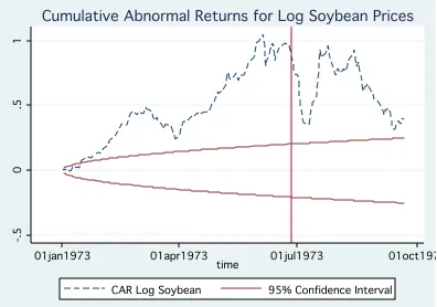
Figure 2.4 Cumulative Abnormal Returns for Log(Soy) . . . 34

Figure 2.5 Cumulative Abnormal Returns for Log(Corn) . . . 35

Figure 2.6 Monthly Prices of Domestic Soy and Export Soy . . . 36

Figure 2.7 Monthly Log Relative Prices of Domestic Soy and Export Soy . . 37

Figure 2.8 Forecasted Monthly Prices from VECM with Observed Prices

(Do-mestic and Exported Soybeans) . . . 38

Figure 2.9 Cumulative Abnormal Returns for Monthly Domestic Log Soybean

Prices . . . 39 Figure 2.10 Cumulative Abnormal Returns for Monthly World Log Soybean

Prices . . . 40

Figure 2.11 Monthly Log Prices of Soy and Corn . . . 41

Figure 2.12 Monthly Log Relative Prices of Soy and Corn . . . 42

Figure 2.13 Forecasted Monthly Prices from VECM with Observed Prices (Soy-beans and Corn) . . . 43

Figure 3.1 Pre Euro Ex Ante Expected Real Interest Rates and Ex Post Real

Interest Rates . . . 77

Figure 3.2 Pre Euro Distributions and Kernel Densities for Real Interest Rate

Differentials . . . 78

Figure 3.3 Pre Euro Distributions and Kernel Densities for First-Differenced

Real Interest Rate Differentials . . . 79

Figure 3.4 Pre Euro ECM Copulas . . . 80

Figure 3.5 Pre Euro Estimated Copula Function Mean Relationships (From

Nonparametric Marginals):C(∆(r_ti−rj_t),(r_ti₋₁−rj_t₋₁)) . . . 81

Figure 3.6 Derivatives of Standard Linear VEC Models and Copula Models . 82

Figure 3.7 Pre Euro Ex Ante Expected Real Interest Rates and Ex Post Real

Interest Rates . . . 83 Figure 3.8 Post Euro Distributions and Kernel Densities for Real Interest Rate

Differentials . . . 84

Figure 3.9 Post Euro Distributions and Kernel Densities for First-Differenced

Real Interest Rate Differentials . . . 85

Figure 3.10 Post Euro ECM Copulas . . . 86

(13)

Figure 3.11 Post Euro Estimated Copula Function Mean Relationships (From

Nonparametric Marginals):C(∆(r_ti−rj_t),(r_ti₋₁−rj_t₋₁)) . . . 87

Figure 3.12 Derivatives of Standard Linear VEC Models and Copula Models . 88 Figure 4.1 Number of Swine Farms by County in North Carolina . . . 109

Figure 4.2 Number of Hogs by County in North Carolina . . . 110

Figure 4.3 Concentration of Swine Farms by County in North Carolina . . . 111

Figure 4.4 All Years - MRSA Infections by County in North Carolina . . . . 112

Figure 4.5 2007 MRSA Infections by County in North Carolina . . . 113

Figure 4.10 All Years - MRSA Incidence Rate per 100,000 People by County in North Carolina . . . 118

Figure 4.11 2007 MRSA Incidence Rate per 100,000 People by County in North Carolina . . . 119

(14)

Chapter 1 Introduction

The following dissertation is broken in to three chapters of work. Each chapter delves

into a separate topic. Below are brief descriptions of each chapter.

1.1 Price Impact of an Embargo - The 1973 Soybean

Embargo in the United States

In 1973, soybeans in the United States were in short supply and prices were increasing

rapidly. The failure of the Peruvian anchovy catch in 1972 dramatically decreased the

availability of high-protein feed for livestock and thereby greatly increased demand for

soybean meal, a high-protein substitute in livestock feed. In January 1973, the USDA

released restrictions on ”set-aside” cropland to help ease the tensions in the market and

increase the production of soybeans. To make matters worse, flooding hindered planting

in the spring of 1973. The U.S. dollar was devalued by approximately ten percent on

(15)

February 15, 1973, contributing to a marked increase in foreign demand for U.S. exports.

As an attempt to stabilize prices and ensure adequate domestic supply, the United States

implemented an export embargo of soybeans, cottonseed and their byproducts on June

27, 1973. The response from importers of these goods was so intense, the embargo was

swiftly lifted less than one week later, on July 2, 1973. The embargo was replaced with

an export-licensing system that was discontinued on September 21, 1973.

I follow a similar econometric model to that of Carter and Smith (2007) in their

analysis of the effect of a food scare due to genetically modified corn not approved for

human consumption being found in the food supply. As in Carter and Smith (2007), I use

a relative price of a substitute good method to estimate the price impact of the embargo.

I compare the prices of soybeans to those of a primary substitute, corn. Corn is a valid

substitute for soybeans due to the fact that they are production substitutes as well as

both are used primarily for animal feed. Also, corn was not affected by the embargo in

1973.

The Carter and Smith relative price of a substitute method exploits the time series

nature of the price of a commodity relative to the price of a substitute good to infer the

price impact of an event that did not impact the substitute good. This allows general

market fluctuations to be accounted for without the need for a formal structural supply

and demand model to be developed. To see the relative price dynamics of the two goods,

the relative price of the two goods must be stable prior to the event of interest. Once

shown stable, any change in the relative price implies a change in the underlying supply

and demand relationship. This allows for a direct estimation of the price impact of the

(16)

I apply time-series analysis techniques appropriate for nonstationary and potentially

cointegrated price series in measuring the impacts of the embargo on equilibrium price

relationships. The ”event study” analysis begins with an analysis of long-run structural

breaks at known and unknown joint points. To this end, I apply a conventional Chow

test for known structural breaks as well as the structural change tests of Hansen (1992),

Hansen (2001), Andrews, Lee and Ploberger (1996), Ploberger and Kramer (1992), and

Bai and Perron (1998). The latter tests are appropriate when the timing of a structural

break is unknown. In such a case, standard Chow-type tests have nonstandard

distribu-tions due to the presence of parameters that are unidentified under the null hypothesis of

no structural break. Upon confirming the presence of a statistically significant structural

break, I undertake estimation that identifies the multiple regimes corresponding to the

periods before and after the embargo.

1.2 Modeling Nonlinear Dynamic Linkages Among

Real Interest Rates

The real interest rate parity (RIP) hypothesis is one of the tenets of international

eco-nomics. Under RIP, well-functioning capital markets would allow for national real interest

rates to be tied to a world interest rate that is determined in the world credit market.

Due to the development of financial markets over the last few decades through removal

of capital controls and other investment barriers, it is likely that capital markets are

more integrated now than in the past. This is important for policy makers, especially in

countries that are small relative to the world credit market, because it ties a country’s

(17)

policy instrument to a world interest rate, thus limiting their abilities to effectively enact

policy independently.

I add to the literature by analyzing the dynamic linkages between real ex ante interest

rates using multivariate threshold models and copulas. First, I follow Frankel (1982) in

his calculation of ex ante real interest rates by deflating the nominal rate by a measure

of the ex ante inflation rate. I apply tests for nonstationarity and cointegration. Then,

I use a threshold model to analyze the dynamic linkages of various countries’ ex ante

real interest rates. To begin, I consider Markov switching models and threshold models

examined by Krolzig (1997) and Tsay (1998) respectively.

Finally, I develop copula-based models that consider the joint distribution of different

national interest rates. This allows attention to be given to the nature of the jointness or

correlation between these interest rates. I allow for the correlation to be state-dependent

and depend on market conditions at any point in time. This is analogous to the

regime-switches in the above models. Copula models use a copula to tie together two marginal

probability functions that may (or may not) be related to one another.

The copula method offers an alternative approach to representing the multivariate

distribution in terms of its dependent marginals. In the case of interest rate parity, the

degree of dependence that characterizes relationships in the tails of the distribution is

of particular relevance. The different types of copulas capture different aspects of this

behavior. To see which copula models fit best, I utilize sequential maximum likelihood

estimation of the copula model for each pair of interest rates. The optimal copula

func-tion(s) for each pair are then chosen using the minimized value of the Bayesin information

(18)

den-sities associated with higher-ordered, multivariate copula models of the elliptical and

Archimedean families as well as in vine copulas.

In this paper, I utilize many nonlinear and nonparametric techniques for assessing

the dynamic linkages in international interest rates. These methods show the level of

integration within the market and stress the level to which policy makers have the ability

to independently influence their home country’s interest rate.

1.3 A Spatial Analysis of MRSA and Livestock Farms

In recent years, there have been numerous headlines about ”Superbugs.” These infections

exhibit antibiotic resistance and are increasingly difficult to treat. Staphylococcus aureus

is a broad grouping of bacteria that tend to live inside the nose and on the skin. Most

of the time it is completely harmless and people don’t realize they are carrying what is

known as a colonization of the bacteria. This bacteria is easily spread from person to

person. Some strains of Staphylococcus aureus exhibit a resistance to a number of

an-tibiotics including methicillin. This is where Methicillin-resistant Staphylococcus aureus

(MRSA) gets its name. MRSA was first reported in 1961, shortly after methicillin was

introduced as treatment for strains that had developed a penicillin resistance. MRSA’s

origins were in hospitals, and it was mostly a hospital-acquired infection (HAI). In the

decades following its discovery, hospital-acquired MRSA (HA-MRSA) strains have

be-come resistant to a myriad of commonly used antibiotics. In the last twenty years, many

people have been increasingly diagnosed with MRSA without having had contact with

a hospital setting. These strains are known as community-acquired MRSA (CA-MRSA).

(19)

Currently, MRSA kills more people each year than AIDS.

MRSA can also be spread between humans and animals from close contact. This has

actually been found in some increasingly common strains, specifically ST398. The first

documented case of ST398 was in the early 2000s in the Netherlands. This is especially

noteworthy since the Dutch have incredibly low levels of HA-MRSA. This strain has been

found on many swine farms in Europe, Canada and the United States. Specifically, in

Canada, 20 percent of swine farm workers, 25 percent of pigs and 45 percent of farms

were reported to be colonized with various strains of MRSA. In all countries with MRSA

colonization in swine farms, the workers on those farms and their families are found to

test positive in large proportions. Strains of MRSA commonly found on swine farms

and in swine farm workers (specifically ST398), have resistance to many antibiotics, but

one that stands out is tetracycline. Tetracycline is used often in the raising of hogs and

not often used in humans. This has led some researchers to postulate that this strain of

MRSA developed its antibiotic resistance on said farms.

The goal of this paper is to test whether there is a link between the increasing presence

of MRSA on swine farms with the uptick in CA-MRSA using North Carolina hospital

discharge data in logistic regression models and county level data using count and

frac-tional models. The results of this paper show whether a person’s proximity to swine

farms and concentration of said swine farms is related to their likelihood of contracting

CA-MRSA. This has many implications for public health officials. With the increasing

numbers of CA-MRSA infections and the high number of people dying from MRSA

(20)

Chapter 2 The Price Impact of an Embargo:

The 1973 Soybean Embargo in the

United States

2.1 Introduction

In mid-1973, soybeans in the United States were in short supply and prices were increasing

quickly. The failure of the Peruvian anchovy catch in 1972 dramatically decreased the

availability of high-protein feed for livestock and thereby greatly increased demand for

soybean meal, a high-protein substitute in feed. In January 1973, the USDA released

restrictions on “set-aside” cropland1 to help ease the tensions in the market and increase

1_{“Set-aside was an agricultural policy that required farmers to set aside a certain percentage of their}

total planted acreage to devote to approved conservation uses. The policy has not been used since the late 1970s and authority for “set-aside” was eliminated by the 1996 Farm Bill.

(21)

the production of soybeans. To make matters worse, flooding hindered planting in the

spring of 1973. Furthermore, the U.S. dollar was devalued against major trading partners

by approximately ten percent on February 15, 1973, contributing to a marked increase

in foreign demand for U.S. exports.

As an attempt to stabilize prices and ensure adequate domestic supply, the United

States implemented an export embargo of soybeans, cottonseed and their byproducts on

June 27, 1973. This was carried out under the ”short supply” provision of The Export

Administration Act of 1969, which delegated the authority to control exports from the

United States for three purposes:

“(A) to the extent necessary to protect the domestic economy from the

exces-sive drain of scarce materials and to reduce the serious inflationary impact of

abnormal foreign demand, (B) to the extent necessary to further significantly

the foreign policy of the United States and to fulfill its international

respon-sibilities, and (C) to the extent necessary to exercise the necessary vigilance

over exports from the standpoint of their significance to the national security

of the United States.”2

The response from importers of these goods was so intense, namely Japan and European

countries, the embargo was swiftly lifted less than one week later, on July 2, 1973.

The embargo was replaced with an export-licensing system. Export licenses were

issued against each contract for 50 percent of unfilled soybean contracts and 40 percent of

unfilled meal and cake contracts. This strict licensing system was relaxed for soybean meal

(22)

and cake in August and in September for soybeans. Licensing was altogether discontinued

on September 21, 1973. This coincided with the new soybean harvest in the United States.

This embargo was not only short; it actually did not impact any contracted shipments

to the largest importer of United States’ soybeans, Japan. In 1973, Japan, in the midst

of an already highly inflationary period, obtained over 88 percent of its soybean imports

from the United States. This was approximately 84 percent of its total supply of soybeans.

A disruption in supply of soybeans from the United States would have been detrimental

to Japan as soybeans were (and still are) a major staple of the country’s diet. It was also

used extensively in animal feed. It is important to note that there are differences in

feed-grade and food-feed-grade soybeans. Six percent of Japan’s supply of soybeans was produced

domestically at this time. In addition, the United States produced approximately 68

percent of the world’s soybeans during this period.

The embargo came without warning for Japan, and there were fears about future

disruptions to trade between the United States and Japan. To ease tension, even after

the end of the embargo and licensing period, Secretary of Agriculture, Earl Butz, visited

the Japanese Minister of Agriculture, Tadao Kuraishi, in Tokyo in April 1974 to guarantee

the Japanese government of the reliability of American exports. These guarantees were

followed by the Butz-Abe Agreement in 1975; a bilateral agreement that set minimum

annual quantities of wheat, feed grains and soybeans the United States would supply to

Japan over the 1976-1978 period. All of these minimum quantities were exceeded in all

of the years of the agreement.

Since the embargo was so short and did not impact any contracted shipments, I

investigate whether or not it was still able to impact the price of soybeans. As it turns

(23)

out, the embargo was able to temporarily stabilize prices, but once it’s short duration

was discovered, uncertainty intensified immensely, and prices increased even more.

Embargoes are relatively rare in United States’ history, but are more common in

other countries, especially developing countries. In this particular case, the United States

enacted a ban on the trade of soybeans and its byproducts as well as cottonseed and

its byproducts with all countries. This was put into effect due to a shortage of soybeans

at home as well as an attempt to stabilize prices. This was essentially a food security

issue. Some embargoes are put in to place for political reasons as opposed to food security

reasons. The issue with embargoes is that they cause increased volatility in a market. They

also cause the enacting country to be viewed as an unreliable supplier. Thinking about

this from the other country’s side (in this case think of Japan), these extreme non-tariff

barriers are a justification for the role of government intervention in agricultural markets.

Japan had very little domestic production of soybeans and essentially one supplier. An

argument could be made for government intervention to encourage increased growth at

home and for the diversification of suppliers.

In the following sections, I explore the price impact of the embargo on soybean prices.

Section 2.2 details the background and methodology, Section 2.3 presents the data and

results, Section 2.4 continues with a discussion of the results and Section 2.5 concludes

(24)

2.2 Background and Methodology

I follow a similar econometric model to that of a differnce-in-differences model. I use a

relative price of a substitute good method to estimate the price impact of the embargo,

as in Carter and Smith (2007). I compare the prices of soybeans to those of a primary

substitute, corn. Corn is a valid substitute for soybeans due to the fact that they are

production substitutes, as well as both used primarily for animal feed. Corn is used as a

calorie supplement and soymeal is used as a protein source. Also, corn was not affected

by the embargo in 1973. Essentially, corn is used as the control in this model.

The relative price of a substitute method exploits the time series properties of the

price of a commodity considered relative to the price of a substitute good to infer the

price impact of an event that did not impact the substitute good. This allows general

market fluctuations to be accounted for without the need for a formal structural supply

and demand model to be developed. To see the relative price dynamics of the two goods,

the relative price of the two goods must be stable prior to the event of interest. Once

shown stable, any change in the relative price implies a change in the underlying supply

and demand relationship. This allows for a direct estimation of the price impact of the

event.

I apply time-series analysis techniques appropriate for nonstationary and potentially

cointegrated price series in measuring the impacts of the embargo on equilibrium price

relationships. The ”event study” analysis begins with an analysis of long-run structural

breaks at known and unknown joint points. To this end, I apply a conventional Chow

test for known structural breaks as well as the structural change tests of Hansen (1992),

Hansen (2001), Andrews, Lee and Ploberger (1996), Ploberger and Kramer (1992), Bai

(25)

and Perron (1998) and Bai and Perron (2003). The latter tests are appropriate when the

timing of a structural break is a priori unknown. In such a case, such Chow-type tests

have nonstandard distributions due to the presence of parameters that are unidentified

under the null hypothesis of no structural break.

Upon confirming the presence of a statistically significant structural break, I

under-take estimation that identifies the multiple regimes corresponding to the periods before

and after the embargo. The dynamics of adjustments to market shocks across different

commodity markets are evaluated. The embargo and its implications for the substantial

rise in the prominence of Brazilian soybean exports and the concomitant adjustments

realized in the United States’ export market are discussed in Section 2.4.

2.3 Data and Results

My analysis uses daily cash closing price data from the Chicago Board of Trade for

Chicago #2 soybeans and Chicago #2 yellow corn. The price of soybeans tended to

move with corn prices before the embargo. The relative prices were very stable. Figure

1 shows the prices of soybeans and corn in log terms prior to the embargo. In 1962,

the soybean harvest was approximately 19% of the corn harvest and by 1972 it was

approximately 27%. Soybean production increased about 69% during this period while

corn increased only 15%. Even as production changed drastically, relative prices stayed

rather stable showing that demand for soybeans and corn was elastic, implying close

substitutability. From 1962 to 1970 the average log price difference between soybeans and

(26)

was 1.1551, or about 115.51%. Thus, soybeans went from having a 79.66% premium over

corn to having a 115.51% premium.

To illustrate the long-run stability in the relative price of soybeans to corn, prior to

the embargo, I show that absolute soybean and corn prices were cointegrated with a (1,

-β) cointegrating vector. A pair of time series data are cointegrated if they have a common

stochastic trend as shown in Engle and Granger (1987). When viewed separately, each

series exhibits a stochastic trend or a unit root, but when viewed as a linear combination

of the series, there is no unit root or trend. Here, the cointegration between soybeans and

corn can be represented by the following model:

st=µ+βct+zt (2.1)

wherestdenotes the log price of soybeans,ctis the log price of corn, andztis a stationary

error term. Now, I apply the augmented Dickey-Fuller test to the log price of soybeans

and corn separately to demonstrate the presence of a unit root in both series, then to the

log relative price of soybeans to corn to show the lack of a unit root, thus showing the

two series are cointegrated. The results of these tests using data prior to the embargo

(from 1960 - 1972) are presented in Table 2.1. The tests show that the prices of soybeans

and corn were cointegrated prior to 1973.

To start with the breaks testing, I run a standard Chow test for one known break at

the time of the embargo. Based on the results, I reject the null hypothesis of no structural

break at the time of the embargo. Next, I use the structural breaks tests of Bai and Perron

(1998 and 2003) to determine whether or not the log relative price stayed stable beyond

1972, through the period containing the embargo. To do this, I expand the sample of

(27)

data to include the embargo, through 1975. A break in the relative price of soybeans to

corn would indicate that whatever shock caused the break had a lasting impact on the

long-run pricing relationship. Since the data were cointegrated prior to 1973, this would

suggest that there were no pre-1973 breaks, otherwise the series would not have been

cointegrated. Thus, the breaks tests provide a robustness check on the aforementioned

cointegration results.

First, break dates are determined using an algorithm developed by Bai and Perron

(2003). The algorithm computes estimates of break points that are global minimizers

of the sum of squared residuals based on the principle of dynamic programming. For

each number of breaks, m, parameters are estimated and the resulting residual sum of

squares is stored. For each number of breaks, the estimated regression that minimizes

the residual sum of squares is selected. Then to select the number of breaks, I use the

Bayesian Information Criterion (BIC) from the estimated regression for each number of

breaks. The BIC is minimized at one break as shown in Table 2.2. I also test for breaks

using sequential sup-F tests and recursive estimates tests and these tests confirm the

presence of just one break3_{. This procedure provides strong evidence of one break in}

early July 1973. This is after the announcement (and end) of the embargo.

The finding of a break in mid July is corroborated by Figure 2.2, which shows the log

relative price of soybeans and corn through the entire sample. The relative price stayed

rather stable through the pre-embargo period, then around the break date found by the

Bai and Perron process, which is referenced by the vertical line, the log relative price

increased substantially.

(28)

Next, I want to analyze the price impact of this event. To do so, I form a vector error

correction model (VECM) for forecasting. The VECM is:

∆st=αszt−1+γs(L)∆st−1+δc(L)∆ct−1+st (2.2)

∆ct=αczt−1+γc(L)∆ct−1 +δs(L)∆st−1+st

where γs(L), δs(L), γc(L), δc(L) are polynomials in the lag operator andzt =st−ct−µ

is the error correction term. The parameters αsand αcare terms measuring the response

of soybean and corn prices to deviations from the long-run trend. The closer these values

are to zero, the longer it takes for the series to return to the long-run trend after a shock.

The results of the estimation of equation (2.2) are in Table 2.3 using data through 1973

(before the embargo).

The error correction parameter for soybeans,αs, is -0.00016, which is not significantly

different from zero. The error correction parameter for corn,αc, is 0.0039. This indicates

that on average the daily price of corn changes to correct any deviation from long-run

trend by 0.39%. This is very small and suggests a slow reversion, but it is significantly

different from zero. This suggests that soybean and corn can deviate from the long-run

stable relationship for long periods of time, but eventually retire to a stable equilibrium

relationship. Calculating a half-life from the error correction parameter for corn, it takes

178 days, approximately 35 to 36 weeks for prices to return to the long-run stable trend.

Using the estimates from the VECM, I compute forecasts of the log prices of

soy-beans and corn over the window of the embargo and beyond. The abnormal returns are

calculated as the difference between the forecasted values and the observed values as

(29)

ARs

t = ∆st−∆ˆst−1 for soybeans and ARct = ∆ct−∆ˆct−1 for corn. The results of this

are shown in Figure 2.3. If one sums over the window of interest, cumulative abnormal

returns are revealed as

CARs =

k

X

t=s

(∆st−∆ˆst−1) =sk−sˆk (2.3)

CARc =

k

X

t=s

(∆ct−∆ˆct−1) = ck−ˆck

where s is the start of the window and k is the end. Therefore, the CAR is the error in

forecast of soybean or corn prices at the end of the window. Note that my definition of

CAR is not the same as traditional event studies, but better fits the analysis performed

in this paper. The CAR for soybeans and corn with confidence intervals are presented

in Figure 2.4 and 2.5, respectively. Both corn and soybean prices are well above their

forecasted values for the whole period of the embargo and export license system, but

until mid-September, the CAR of soybeans was much above the CAR of corn. On the

day that the embargo was enacted, the CAR of the log price of soybeans was 0.8893 while

the CAR of the log price of corn was only 0.4008. By July 5th, days after the embargo

officially ended, the CAR of the log price of soybeans was down to 0.4089, very close to

corn which was 0.3501. It would appear that the embargo was able to calm some of the

drastic rise in domestic prices. After the end of the embargo and the start of the export

licensing system, both corn and soybean prices increased. The CAR for soybeans show

that on average the log price of soybeans was approximately 0.5235 above its predicted

(30)

Next, I run the whole process again with soybean prices received by farmers from

the USDA National Agricultural Statistics Service (NASS) and with Rotterdam, c.i.f.

monthly soybean prices from the World Bank. These data span from January 1960

through December 1989 to ensure a substantial number of observations.

The Rotterdam monthly soybean prices with the NASS soybean prices reveal similar

results. The two series are plotted in Figure 2.6 with the embargo month highlighted.

The results of Augmented Dickey-Fuller tests are in Table 2.4. The log of domestic

monthly soybean prices and the log of Rotterdam monthly soybean prices both show

the presence of a unit root, but the log relative price of the two series does not have

a unit root and are therefore the prices are cointegrated, thus implying a cointegrating

vector of [1,−1]. The Bai and Perron test shows one break in April 1973. This is shown

in Figure 2.7. Once again, the vector error correction model estimates are presented

in Table 2.5. The error correction parameter for domestic soybeans, αd, is -0.2895 and

is significant at a ten percent level. This indicates that the average monthly price of

domestic soybeans changes to correct any deviation from the long-run trend by about

-28.95%. The error correction parameter for Rotterdam soybeans, αe, is 0.4185, which

is not statistically different from zero. The half-life calculation from the error correction

parameter on domestic soybeans implies that it takes almost 3 months for prices to return

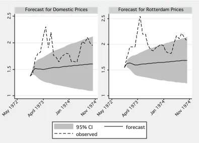
to the long-run stable relationship. The forecasts for monthly prices during the period of

the embargo from the VECM are in Figure 2.8.

The cumulative abnormal returns for domestic soybeans and Rotterdam soybeans are

in Figures 2.9 and 2.10, respectively. These show something quite interesting. In April

1973, when the break was estimated by the Bai and Perron tests, the CAR for domestic

(31)

log soybean prices was 0.3063 and 0.3410 for Rotterdam prices. In May both CAR’s had

almost doubled to 0.5999 for domestic prices and 0.6621 for Rotterdam prices. By June,

when the embargo was put into place, the domestic CAR increased to only 0.7824, while

the Rotterdam CAR increased to 0.9317. Following this marked increase for both sets

of prices, July’s domestic CAR was 0.3743 and 0.5750 for Rotterdam prices. This would

appear to indicate that the embargo stabilizing domestic prices, while not impacting the

Rotterdam price as much.

Rotterdam represents a global price discovery point for soybeans. In the 1973/1974

production year the United States produced approximately 78 percent of the soybeans

in the world according to the USDA Foreign Agricultural Service. As the United States

was the majority producer of soybeans, it is not surprising that changes in the price

of United States’ soybeans affected the Rotterdam price of soybeans. Interestingly, the

United States’ market share for soybeans started to drop in 1975, coinciding with the

advent of the Brazilian soybean market, in which Japan was a major investor.

Finally, as a robustness check, I run the analysis on NASS soybean and corn monthly

prices. The data span from January 1960 through December 1989 as with the Rotterdam

analysis. Figure 11 plots the monthly log prices of soybeans and corn. Table 6 presents

the results of the Augmented Dickey-Fuller tests. Both the log of soybean monthly prices

and the log of monthly corn prices exhibit a unit root, but the log difference of the

two series do not, thus suggesting that they are cointegrated series with a cointegrating

vector of [1,−1]. It is clear from the figure that there is indeed a structural break in the

relationship between the prices. The results of the breaks tests are remarkably similar to

(32)

Perron test for unknown breaks reveals one break in the log relative price of soybeans

and corn. This break is in March 1973, just before the embargo. The break is plotted in

the log relative prices in Figure 2.12. This pre-embargo break in monthly prices further

proves a substantial change in the conditions of the soybean market. The fact that it

occurs before the embargo implies that the market was already in the process of a change

before the embargo was implemented. This could be the policy being anticipated by the

market.

The vector error correction model estimates are presented in Table 2.7. The error

correction parameter for soybeans, αs, is -0.139, which is not significantly different from

zero. The error correction parameter for corn,αc, is 0.0934. This indicates that on average

the monthly price of corn changes to correct any deviation from long-run trend by 9.34%.

The forecasts from the VECM for the period of the embargo are in Figure 2.13. The

half-life from the error correction parameter for corn implies that it takes between 7 and 8

months for prices to return to the long-run stable relationship.

2.4 Discussion

In this paper, I have used the relative price of a substitute method developed by Carter

and Smith (2007) to show the impact of a very short embargo on the price of soybeans.

This approach is quite novel, and allows for estimation of a price impact without the

need for a formal structural supply and demand model. This is attractive because any

misspecification in the structural model will bias the results. This method, by using a

substitute good, allows for general market fluctuations to be accounted for while teasing

(33)

out the event that happened to the commodity of interest.

I use the relative price of a substitute good method to estimate the price impact of this

embargo with daily price data. Initially, using corn as a substitute not impacted by the

embargo, I am able to capture the relative change in the price of soybeans. I apply

time-series analysis techniques appropriate for nonstationary and cointegrated prices time-series in

measuring the impacts of the embargo on equilibrium price relationships. Testing for

long-run structural breaks at known and unknown points is done, followed by the estimation

of a vector error correction model that allows the creation of forecasts for the prices had

such a break not occurred. The forecast error from this model is used to estimate the

price impact of the embargo. The process is repeated with monthly prices for corn and

soybeans as well as with monthly domestic and export prices for soybeans.

The VECM models in all cases above forecasted soybean prices to be lower than what

happened in reality. The daily data showed a break happening after the embargo had

ended, but still during the export licensing program. The monthly data for soybeans and

corn showed the break happening just before the embargo began, similar to the results

from the Rotterdam and domestic soybean analysis. These results show that there was

indeed a structural change in the market for soybeans around the time of the embargo

being enacted.

The embargo did in fact have an impact on the price of soybeans, a statistically

significant one at that. From the daily price analysis, the cumulative abnormal return

calculated from the vector error correction model of the log price of soybeans was much

above that of corn. On the day that the embargo was enacted, the CAR of soybeans

(34)

embargo was lifted, the CAR of soybeans was 0.4089, close to the CAR of corn, 0.3501.

After the embargo the CAR of soybeans increased. From January 1973 through the end

of the export licensing system, the CAR for soybeans and corn show that on average the

log price of soybeans was approximately 0.5235 above its predicted value and the average

log price of corn was approximately 0.2531 above its predicted value. These results are

very similar to the monthly price analysis for both soybean and corn prices as well as the

Rotterdam and domestic soybean prices.

The relationship between the United States and Japan was disturbed by the

im-position of an embargo in June of 1973. Since the embargo came without warning for

Japan, there were fears about further disruptions to trade between the two countries.

Even though efforts were made to minimize the impacts on the Japanese, Japan made

strategic investments to diversify the supply of soybeans in the future by investing heavily

in the infant Brazilian soybean market. Brazil now is second only to the United States

in soybean production.

Using the soybean embargo as a starting point, I looked to other embargoes by the

United States. The wheat embargo to the Soviet Union in 1980 is one example. I ran the

above analysis on this event and found that it did not impact wheat prices (using corn as

a substitute) in the way that soybeans were impacted. Wheat and corn were cointegrated

over the period leading up the the wheat embargo. With this result in hand, the relative

price of a substitute good method revealed that there was in fact no price impact from

the wheat embargo. First, I used a standard Chow test for one known break at the time

of the embargo. I was unable to reject the null hypothesis of no structural break at the

time of the embargo against the Soviet Union. To ensure there were no breaks around this

(35)

time, I used the Bai and Perron test for unknown structural breaks. Again, I was unable

to reject the first null hypothesis of no structural break over the whole time period which

was from 1960 through 1999. This makes sense because the embargo only was placed

against one country and there were many options for wheat for the Soviet Union outside

of the United States such as Canada, Argentina, and Australia. There are also indications

that the Soviet Union was able to skirt the embargo by the use of intermediaries. This

embargo, unlike the soybean embargo, was put in to place for political reasons as well.

2.5 Concluding Remarks

The purpose of this paper was to test if the soybean embargo of 1973 had a price impact

on the market price of soybeans even though it did not impact any contracted shipments.

While the results show that the embargo was able to stabilize prices for a very short period

of time, the aftermath was substantially higher prices. The embargo and the export

licensing system appear to have increased uncertainty even more than the other market

conditions and therefore caused prices to increase further. This shows that policy makers

should exercise caution when enacting trade policies of this sort. Even short embargoes

that do not impact any contracted shipments are able to exacerbate uncertainty and

cause our trading partners to seek diversity in sources for necessities like Japan did with

investing in the Brazilian soybean market.

Embargoes are relatively rare in United States’ history, but are more common in

other countries, especially developing countries. In this particular case, the United States

(36)

byproducts with all countries. This was put into effect due to a shortage of soybeans at

home as well as an attempt to stabilize prices. This was essentially a food security issue.

Some embargoes are put in to place for political reasons as opposed to food security

reasons. The issue with embargoes is that they cause increased volatility in a market.

They also cause the enacting country to be viewed as an unreliable supplier. The purpose

of this paper was to analyze whether or not this particular embargo was able to do what

it set out to: stabilize prices. It did.

The implications for unexpected trade embargoes are large and in the future I plan to

analyze the rise in the Brazilian soybean market and its impact on the United States’

soy-bean market. Using a structural model, I plan to investigate how non-tariff barriers such

as embargoes impact the market share of countries’ exports for different commodities,

and if barriers to one commodity affect other commodities.

(37)

Table 2.1: Cointegration Tests on Daily Prices

Test Statistic 5% Critical Value Conclusion

Log Soybeans -1.34 -2.86 Unit Root

Log Corn -2.71 -2.86 Unit Root

Log Difference -2.92 -2.86 Cointegrated

Note: All ADF tests include an intercept, no trend, and 5 lags (as determined by FPE,

(38)

Table 2.2: Determination of Number of Structural Breaks

Number of Breaks BIC

0 -21,749.29

1 -21,849.36

2 -21,833.15

3 -21,782.34

4 -21,734.07

5 -21,682.87

Note: Modeled using the log difference of soybeans and corn with 5 lags (as determined

by FPE, AIC and LR).

(39)

Table 2.3: Pre-Embargo Vector Error Correction Model Estimates For Daily Prices

Parameter Soybeans Corn

α -0.0016 0.0039**

γ1 -0.0337* 0.0153

γ2 -0.0465** 0.0105

γ3 0.0486* 0.0180

γ4 0.0059 0.0552**

δ1 0.0292 0.0438**

δ2 0.0300* -0.0170

δ3 0.0094 -0.0078

δ4 0.0094 -0.0146

Note: Sample period is 1960-1972. Estimation by Johansen’s (1995) maximum likelihood

(40)

Table 2.4: Cointegration Tests for Monthly Domestic and Rotterdam Soybean Prices

Log Domestic Soybeans -1.809 -2.887 Unit Root

Log Rotterdam Soybeans -1.104 -2.887 Unit Root

AIC and LR). Log Difference is log(Soybeans/Corn).

(41)

Table 2.5: Pre-Embargo Vector Error Correction Model Estimates for Monthly Domestic and Rotterdam Soybean Prices

Parameter Domestic Soybeans Rotterdam Soybeans

α -0.2895* 0.4185

γ1 0.0449 0.5580**

γ2 -0.3202** -0.0316

δ1 0.5361** -0.0511

δ1 0.1548 -0.1231

(42)

Table 2.6: Cointegration Tests for Monthly Soybean and Corn Prices

Log Soybeans -1.409 -2.887 Unit Root

Log Corn -2.448 -2.887 Unit Root

AIC and LR). Log Difference is log(Soybeans/Corn).

(43)

Table 2.7: Pre-Embargo Vector Error Correction Model Estimates for Monthly Soybean and Corn Prices

Parameter Soybeans Corn

α -0.139 0.0934**

γ1 0.543** 0.278**

γ2 -0.3114** -0.1271

γ3 0.1395 0.1760**

δ1 -0.0136 0.1473*

δ2 -0.0155 -0.0216

δ3 -0.0513 -0.1029

(44)

4.5 4. 5 4.5 5 5 5 5.5 5. 5 5.5 6 6 6 01jul1962 01jul1962 01jul1962 01jan1963 01jan 1963 01jan1963 01jul1963 01jul1963 01jul1963 01jan1964 01jan 1964 01jan1964 01jul1964 01jul1964 01jul1964 01jan1965 01jan 1965 01jan1965 01jul1965 01jul1965 01jul1965 01jan1966 01jan 1966 01jan1966 01jul1966 01jul1966 01jul1966 01jan1967 01jan 1967 01jan1967 01jul1967 01jul1967 01jul1967 01jan1968 01jan 1968 01jan1968 01jul1968 01jul1968 01jul1968 01jan1969 01jan 1969 01jan1969 01jul1969 01jul1969 01jul1969 01jan1970 01jan 1970 01jan1970 01jul1970 01jul1970 01jul1970 01jan1971 01jan 1971 01jan1971 01jul1971 01jul1971 01jul1971 01jan1972 01jan 1972 01jan1972 01jul1972 01jul1972 01jul1972 time time time Log Soybean Log Soybean Log Soybean Log Corn Log Corn Log Corn

Log Soybean and Log Corn Prices Pre-Embargo 1962-1972

Figure 2.1: Daily Log Prices Before Event

(45)

July 12, 1973

July 12, 1973 July 12, 1973

.6 .6 .6 .8 .8 .8 1 1 1 1.2 1. 2 1.2 1.4 1. 4 1.4 1.6 1. 6 1.6 Log Difference Log D iff er en ce Log Difference 01jan1960 01jan 1960 01jan1960 01jan1961 01jan 1961 01jan1961 01jan1962 01jan 1962 01jan1962 01jan1963 01jan 1963 01jan1963 01jan1964 01jan 1964 01jan1964 01jan1965 01jan 1965 01jan1965 01jan1966 01jan 1966 01jan1966 01jan1967 01jan 1967 01jan1967 01jan1968 01jan 1968 01jan1968 01jan1969 01jan 1969 01jan1969 01jan1970 01jan 1970 01jan1970 01jan1971 01jan 1971 01jan1971 01jan1972 01jan 1972 01jan1972 01jan1973 01jan 1973 01jan1973 01jan1974 01jan 1974 01jan1974 01jan1975 01jan 1975 01jan1975 time time time

Log Relative Prices (Soybean/Corn) by Day

(46)

6 6 6 6.5 6. 5 6.5 7 7 7 5 5 5 5.5 5. 5 5.5 6 6 6 12/13/72 12/ 13/ 72 12/13/72 2/28/73 2/28/ 73 2/28/73 5/10/73 5/10/ 73 5/10/73 7/24/73 7/24/ 73 7/24/73 10/3/73 10/ 3/73 10/3/73 12/13/72 12/ 13/ 72 12/13/72 2/28/73 2/28/ 73 2/28/73 5/10/73 5/10/ 73 5/10/73 7/24/73 7/24/ 73 7/24/73 10/3/73 10/ 3/73 10/3/73

Forecast for Log Soybean Prices

Forecast for Log Soybean Prices Forecast for Log Soybean Prices

Forecast for Log Corn Prices

Forecast for Log Corn Prices Forecast for Log Corn Prices

95% CI 95% CI 95% CI forecast forecast forecast observed observed observed

Figure 2.3: Forecasted Daily Prices from VECM with Observed Prices

(47)

-.5

-.5 0

0

0 .5

.5

.5 1

1

01jan1973

01jan1973 01jan1973 01apr1973

01apr1973 01apr1973

01jul1973

01jul1973 01jul1973

01oct1973

01oct1973 01oct1973

time

time time

CAR Log Soybean

CAR Log Soybean CAR Log Soybean

95% Confidence Interval

95% Confidence Interval 95% Confidence Interval

Cumulative Abnormal Returns for Log Soybean Prices

(48)

-.2 -.2 -.2 0 0 0 .2 .2 .2 .4 .4 .4 .6 .6 .6 .8 .8 .8 01jan1973 01jan1973 01jan1973 01apr1973 01apr1973 01apr1973 01jul1973 01jul1973 01jul1973 01oct1973 01oct1973 01oct1973 time time time

CAR Log Corn

CAR Log Corn CAR Log Corn

Cumulative Abnormal Returns for Log Corn Prices

Figure 2.5: Cumulative Abnormal Returns for Log(Corn)

(49)

June 1973 June 1973 June 1973 .5 .5 .5 1 1 1 1.5 1. 5 1.5 2 2 2 2.5 2. 5 2.5 01jan1960 01jan 1960 01jan1960 01jan1962 01jan 1962 01jan1962 01jan1964 01jan 1964 01jan1964 01jan1966 01jan 1966 01jan1966 01jan1968 01jan 1968 01jan1968 01jan1970 01jan 1970 01jan1970 01jan1972 01jan 1972 01jan1972 01jan1974 01jan 1974 01jan1974 01jan1976 01jan 1976 01jan1976 01jan1978 01jan 1978 01jan1978 01jan1980 01jan 1980 01jan1980 01jan1982 01jan 1982 01jan1982 01jan1984 01jan 1984 01jan1984 01jan1986 01jan 1986 01jan1986 01jan1988 01jan 1988 01jan1988 01jan1990 01jan 1990 01jan1990 time time time Rotterdam Rotterdam Rotterdam Domestic Domestic Domestic

Log Rotterdam Soy and Log Domestic Soy Prices by Month

(50)

April 1973 April 1973 April 1973 -.4 -.4 -.4 -.3 -.3 -.3 -.2 -.2 -.2 -.1 -.1 -.1 0 0 0

Log Difference D-R

Log D iff er en ce D -R

Log Difference D-R 01jan1960 01jan 1960 01jan1960 01jan1962 01jan 1962 01jan1962 01jan1964 01jan 1964 01jan1964 01jan1966 01jan 1966 01jan1966 01jan1968 01jan 1968 01jan1968 01jan1970 01jan 1970 01jan1970 01jan1972 01jan 1972 01jan1972 01jan1974 01jan 1974 01jan1974 01jan1976 01jan 1976 01jan1976 01jan1978 01jan 1978 01jan1978 01jan1980 01jan 1980 01jan1980 01jan1982 01jan 1982 01jan1982 01jan1984 01jan 1984 01jan1984 01jan1986 01jan 1986 01jan1986 01jan1988 01jan 1988 01jan1988 01jan1990 01jan 1990 01jan1990 time time time

Log Relative Prices (domestic/export) by Month

Figure 2.7: Monthly Log Relative Prices of Domestic Soy and Export Soy

(51)

1 1 1 1.5 1. 5 1.5 2 2 2 2.5 2. 5 2.5 1 1 1 1.5 1. 5 1.5 2 2 2 2.5 2. 5 2.5 May 1972 May 1 972 May 1972 April 1973 April 1 973 April 1973 Jan 1974 Jan 1 974 Jan 1974 Nov 1974 Nov 197 4 Nov 1974 May 1972 May 1 972 May 1972 April 1973 April 1 973 April 1973 Jan 1974 Jan 1 974 Jan 1974 Nov 1974 Nov 197 4 Nov 1974

Forecast for Domestic Prices

Forecast for Domestic Prices Forecast for Domestic Prices

Forecast for Rotterdam Prices

Forecast for Rotterdam Prices Forecast for Rotterdam Prices

(52)

-.5 -.5 -.5 0 0 0 .5 .5 .5 1 1 1 April 1973 April 1 973 April 1973 May 1973 May 1 973 May 1973 June 1973 June 197 3 June 1973 July 1973 July 1 973 July 1973 Aug 1973 Aug 1 973 Aug 1973 Sept 1973 Sept 197 3 Sept 1973 time time time

CAR Domestic Soybeans

CAR Domestic Soybeans CAR Domestic Soybeans

Cumulative Abnormal Returns for Log(Soybean) Prices

Figure 2.9: Cumulative Abnormal Returns for Monthly Domestic Log Soybean Prices

(53)

-.5 -.5 -.5 0 0 0 .5 .5 .5 1 1 1 April 1973 April 1 973 April 1973 May 1973 May 1 973 May 1973 June 1973 June 197 3 June 1973 July 1973 July 1 973 July 1973 Aug 1973 Aug 1 973 Aug 1973 Sept 1973 Sept 197 3 Sept 1973 time time time

CAR Rotterdam Soybeans

CAR Rotterdam Soybeans CAR Rotterdam Soybeans

Cumulative Abnormal Returns for Log(Rotterdam) Prices

(54)

0 0 0 .5 .5 .5 1 1 1 1.5 1. 5 1.5 2 2 2 2.5 2. 5 2.5 01jan1960 01jan 1960 01jan1960 01jan1962 01jan 1962 01jan1962 01jan1964 01jan 1964 01jan1964 01jan1966 01jan 1966 01jan1966 01jan1968 01jan 1968 01jan1968 01jan1970 01jan 1970 01jan1970 01jan1972 01jan 1972 01jan1972 01jan1974 01jan 1974 01jan1974 01jan1976 01jan 1976 01jan1976 01jan1978 01jan 1978 01jan1978 01jan1980 01jan 1980 01jan1980 01jan1982 01jan 1982 01jan1982 01jan1984 01jan 1984 01jan1984 01jan1986 01jan 1986 01jan1986 01jan1988 01jan 1988 01jan1988 01jan1990 01jan 1990 01jan1990 time time time Log Corn Log Corn Log Corn Log Soybean Log Soybean Log Soybean

Log Corn and Log Soybean Prices by Month

Figure 2.11: Monthly Log Prices of Soy and Corn

(55)

March 1973 March 1973 March 1973 .6 .6 .6 .8 .8 .8 1 1 1 1.2 1. 2 1.2 1.4 1. 4 1.4 1.6 1. 6 1.6 Log Difference Log D iff er en ce Log Difference 01jan1960 01jan 1960 01jan1960 01jan1962 01jan 1962 01jan1962 01jan1964 01jan 1964 01jan1964 01jan1966 01jan 1966 01jan1966 01jan1968 01jan 1968 01jan1968 01jan1970 01jan 1970 01jan1970 01jan1972 01jan 1972 01jan1972 01jan1974 01jan 1974 01jan1974 01jan1976 01jan 1976 01jan1976 01jan1978 01jan 1978 01jan1978 01jan1980 01jan 1980 01jan1980 01jan1982 01jan 1982 01jan1982 01jan1984 01jan 1984 01jan1984 01jan1986 01jan 1986 01jan1986 01jan1988 01jan 1988 01jan1988 01jan1990 01jan 1990 01jan1990 time time time

Log Relative Prices (soybean/corn) by Month

(56)

1 1 1 1.5 1. 5 1.5 2 2 2 2.5 2. 5 2.5 0 0 0 .5 .5 .5 1 1 1 1.5 1. 5 1.5 May 1972 May 1 972 May 1972 April 1973 April 1 973 April 1973 Jan 1974 Jan 1 974 Jan 1974 Nov 1974 Nov 197 4 Nov 1974 May 1972 May 1 972 May 1972 April 1973 April 1 973 April 1973 Jan 1974 Jan 1 974 Jan 1974 Nov 1974 Nov 197 4 Nov 1974

Forecast for Log Soybean Prices

Forecast for Log Soybean Prices Forecast for Log Soybean Prices

Forecast for Log Corn Prices

Forecast for Log Corn Prices Forecast for Log Corn Prices

Figure 2.13: Forecasted Monthly Prices from VECM with Observed Prices (Soybeans and Corn)

(57)

Chapter 3 Modeling Nonlinear Dynamic

Linkages Among Real Interest Rates

3.1 Background

The real interest rate parity (RIP) hypothesis is one of the tenets of international

eco-nomics. Under RIP, well-functioning capital markets would allow for national real interest

rates to be tied to a world interest rate that is determined in the world credit market.

Due to the development of financial markets over the last few decades through the

re-moval of capital controls and other investment barriers, it is likely that capital markets

are more integrated now than in the past. This is important for policy makers, especially

in countries that are small relative to the world credit market, because it ties a country’s

policy instrument to a world interest rate, thus limiting their abilities to effectively enact

policy independently.

A large body of literature has been devoted to the investigation of these international

interest rate linkages. Early studies used conventional regression techniques to test for

Three Essays in Trade and Health.

ABSTRACT

DEDICATION

BIOGRAPHY

ACKNOWLEDGEMENTS

TABLE OF CONTENTS

LIST OF TABLES

LIST OF FIGURES

Chapter 1

Introduction

1.1

Price Impact of an Embargo - The 1973 Soybean

Embargo in the United States

1.2

Modeling Nonlinear Dynamic Linkages Among

Real Interest Rates

1.3

A Spatial Analysis of MRSA and Livestock Farms

Chapter 2

The Price Impact of an Embargo:

The 1973 Soybean Embargo in the

United States

2.1

Introduction

2.2

Background and Methodology

2.3

Data and Results

2.4

Discussion

2.5

Concluding Remarks

Log Soybean and Log Corn Prices Pre-Embargo 1962-1972

Log Soybean and Log Corn Prices Pre-Embargo 1962-1972

Log Soybean and Log Corn Prices Pre-Embargo 1962-1972

Log Relative Prices (Soybean/Corn) by Day

Log Relative Prices (Soybean/Corn) by Day

Log Relative Prices (Soybean/Corn) by Day

Cumulative Abnormal Returns for Log Soybean Prices

Cumulative Abnormal Returns for Log Soybean Prices

Cumulative Abnormal Returns for Log Soybean Prices

Cumulative Abnormal Returns for Log Corn Prices

Cumulative Abnormal Returns for Log Corn Prices

Cumulative Abnormal Returns for Log Corn Prices

Log Rotterdam Soy and Log Domestic Soy Prices by Month

Log Rotterdam Soy and Log Domestic Soy Prices by Month

Log Rotterdam Soy and Log Domestic Soy Prices by Month

Log Relative Prices (domestic/export) by Month

Log Relative Prices (domestic/export) by Month

Log Relative Prices (domestic/export) by Month

Cumulative Abnormal Returns for Log(Soybean) Prices

Cumulative Abnormal Returns for Log(Soybean) Prices

Cumulative Abnormal Returns for Log(Soybean) Prices

Cumulative Abnormal Returns for Log(Rotterdam) Prices

Cumulative Abnormal Returns for Log(Rotterdam) Prices

Cumulative Abnormal Returns for Log(Rotterdam) Prices

Log Corn and Log Soybean Prices by Month

Log Corn and Log Soybean Prices by Month

Log Corn and Log Soybean Prices by Month

Log Relative Prices (soybean/corn) by Month

Log Relative Prices (soybean/corn) by Month

Log Relative Prices (soybean/corn) by Month

Chapter 3

Modeling Nonlinear Dynamic

Linkages Among Real Interest Rates

3.1

Background