Equivalent Keys in Multivariate Quadratic Public Key Systems

Equivalent Keys in

Multivariate

Quadratic Public Key Systems

Christopher Wolf1,2_{, and Bart Preneel}1 1_{K.U.Leuven, ESAT-COSIC}

Kasteelpark Arenberg 10, B-3001 Leuven-Heverlee, Belgium {Christopher.Wolf, Bart.Preneel}@esat.kuleuven.be

or chris@Christopher-Wolf.de http://www.esat.kuleuven.ac.be/cosic/

2_{Ecole Normale Sup´erieure, D´epartement d’Informatique´} 45 rue d’Ulm, F-75230 Paris Cedex 05, France Christopher.Wolf@ens.frorchris@Christopher-Wolf.de

Abstract

Multivariate Quadratic public key schemes have been suggested back in 1985 by Mat-sumoto and Imai as an alternative for the RSA scheme. Since then, several other schemes have been proposed, for example Hidden Field Equations, Unbalanced Oil and Vinegar schemes, and Stepwise Triangular Schemes. All these schemes have a rather large key space for a secure choice of parameters. Surprisingly, the question of equivalent keys has not been discussed in the open literature until recently. In this article, we show that for all basic classes mentioned above, it is possible to reduce the private — and hence the public — key space by several orders of magnitude. For the Matsumoto-Imai scheme, we are even able to show that the reductions we found are the only ones possible, i.e., that these reductions are tight. While the theorems developed in this article are of independent interest themselves as they broaden our understanding of MultivariateQuadratic public key systems, we see applications of our results both in cryptanalysis and in memory efficient implementations ofMQ-schemes.

Keywords: MultivariateQuadratic Polynomials, Public Key signature, Hidden Field Equations, Matsumoto-Imai scheme A, C∗_{, Unbalanced Oil and Vinegar, Stepwise Triangular Systems}

Date: 2005-12-22

1

Initial Considerations

In the last 20 years, several schemes based on the problem ofMultivariateQuadratic equations (or MQfor short) have been proposed. The most important ones certainly are MIA / C∗_{[MI88] and} Hidden Field Equations (HFE, [Pat96b]) plus their variations MIA- / C∗−−_{, HFE-, HFEv, and} HFEv- [KPG99, Pat96a, Pat96b]. Both classes have been used to construct signature schemes for the European cryptography project NESSIE [NES], namely the MIA- variation in Sflash [CGP03], the HFEv- variation in Quartz [CGP01] and the HFE- variation in the tweaked version Quartz-7m [WP04]. Unbalanced Oil and Vinegar schemes [KPG99] and Stepwise Triangular Schemes [WBP04] are also important in practice. While the first is secure with the correct choice of parameters, the second forms the basis of nested constructions like the enhanced TTM [YC04], Tractable Rational Maps [WHL+_{05], or Rainbow [DS05].}

The aim of this paper is to systematically study the question of equivalent keys ofMQ-schemes. At first glance, this question seems to be purely theoretical. But for practical applications, we need memory and time efficient instances of Multivariate Quadratic public key systems. One important point in this context is the overall size of the private key: in restricted environments such as smart cards, we want it as small as possible. Hence, if we can show that a given private key is only a representative of a much larger class of equivalent private keys, it makes sense to compute (and store) only a normal form of this key. Similar, we should construct newMultivariate Quadratic schemes such that they do not have a large number of equivalent private keys but only a small number, preferable only one, per equivalence class. This way, we make optimal use of the randomness in the private key space and neither waste computation time nor storage space without any security benefit.

All systems based onMQ-equations use a public key of the form

pi(x1, . . . , xn) :=

X

1≤j≤k≤n

γi,j,kxjxk+ n

X

j=1

βi,jxj+αi,

with n ∈ Z+ _{variables and m ∈} Z+ _{equations. Moreover, we have 1 ≤ i ≤ m; 1 ≤ j ≤ k ≤ n}

and αi, βi,j, γi,j,k ∈ F (constant, linear, and quadratic terms). We write the set of all such

whereS ∈Aff−1(Fn_{), T ∈Aff}−1_(Fm_{) are bijective affine transformations. Details on affine}

trans-formation are given in Section 2.1). Moreover, we haveP0 _{∈ MQ(F}n_,Fm_{) is a polynomial-vector}

P0 _{:= (p}0

1, . . . , p0m) withmcomponents; each component is a polynomial innvariablesx01, . . . , x0n.

Throughout this paper, we will denote components of this private vector P0 _{by a prime} 0_{. In} contrast to the public polynomial vectorP ∈ MQ(Fn_,Fm_{), the private polynomial vectorP}0 _does

allow an efficient computation ofx0

1, . . . , x0n for giveny01, . . . , y0m. Still, the goal of MQ-schemes

is that this inversion should be hard if the public keyP alone is given. The main difference be-tweenMQ-schemes lies in their special construction of the central equationsP0 _{and consequently} the trapdoor they embed into a specific class ofMQ-problems. An introduction toMultivariate Quadratic public key systems is given in [WP05c].

1.1

Related Work

In their cryptanalysis of HFE, Kipnis and Shamir report the existence of “isomorphic keys” [KS99]. A similar observation for Unbalanced Oil and Vinegar Schemes can be found in [KPG99]. In both cases, there has not been a systematic study of the structure of equivalent key classes. In addition, Patarin observed the existence of some equivalent keys for MIA / C∗ _{[Pat96a] — however, his} method is different from the one presented in this article, as he concentrated on modifying the central monomial rather than using special affine transformations. Moreover, Toli observed that there exists an additive sustainer in the case of Hidden Field Equations [Tol03] but did not extend his result to other Multivariate Quadratic schemes. Additive sustainers will be introduced in Section 3.1. In the case of symmetric ciphers, [BCBP03] used a similar idea in the study of S-boxes. A different angle of the idea of equivalent keys can be found in [HWyCL05] where the authors compute normal forms of the public key. Main reason here is to save some memory in the public but particularily in the private key. Using the techniques suggested in [HWyCL05], the latter can be reduced by up to 50%.

This article is based on the two conference papers [WP05b, WP05a] which deal with the classes MIA, HFE, and UOV. In this article, the proofs have been simplified and also extended to the STS class. In addition, a tightness proof for the case of MIA is given.

1.2

Outline

This paper is organized as follows: after this general introduction, we move on to the necessary mathematical background in Section 2. This includes particularly a definition of the termequivalent keys. In Section 3, we concentrate on a subclass of affine transformations, denoted sustaining transformations, which can be used to generate equivalent keys. These transformations are applied to different variations ofMultivariateQuadratic equations in Section 4. In Section 5, we give a tightness proof for the case of MIA/MIO. This paper concludes with Section 6.

2

Mathematical Considerations

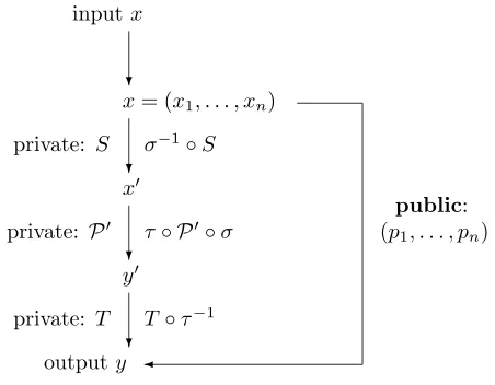
Before discussing concrete schemes, we start with some general observations and definitions. Ob-viously, the most important term in this article is “equivalent private keys”. We give a graphical representation of this idea in Figure 1. We can also express this idea in the following definition:

Definition 2.1 _{We call two private keys}

(S,P0_{, T),( ˜S,P˜}0_,T˜_)∈Aff−1_(Fn_{)× MQ(F}n_,Fm_)×Aff−1_(Fm₎

“equivalent” if they lead to the same public key, i.e., if we have

T◦ P0_{◦S =P = ˜T◦P˜}0_{◦S .}˜

In the above definition, Aff−1_{(·) denotes the class of bijective affine transformations. We give more} details on affine transformations in Section 2.1. In order to find equivalent keys, we consider the following transformations:

Definition 2.2 _{Let (S,P}0_{, T) ∈ Aff}−1_(Fn_{)× MQ(F}n_,Fm_)×Aff−1_(Fm_{), and consider the four}

transformationsσ, σ−1_∈Aff−1_(Fn_{) andτ, τ}−1_∈Aff−1_(Fm_{). Moreover, let}

P =T◦τ−1_{◦τ◦ P}0_◦σ◦σ−1_{◦S . (1)}

We call the pair(σ, τ)∈Aff−1(Fn_)×Aff−1₍Fm_{)“sustaining transformations” for anMQ-system}

inputx

?

x= (x1, . . . , xn)

?

private: S σ−1_◦S

x0

?

private: P0 _{τ◦ P}0_◦σ

y0

?

private: T T◦τ−1 outputy ¾

public: (p1, . . . , pn)

Fig. 1: Equivalent private keys using affine transformationsσ, τ

(S,P0_{, T)for (2.2) and (σ, τ)sustaining transformations. This idea has already been outlined in} Figure 1.

Remark. In the above definition, the meaning of “shape” is still open. In fact, its meaning has to be defined for each MQ-system individually. For example, in HFE (cf Section 4.1), it is the bounding degree d∈ Z+ _{of the polynomial P}0_(X0_{) ∈}E_[X0_{]. In the case of MIA, the “shape” is}

the fact that we have a single monomial with factor 1 as the central equation (cf Section 4.2). In general and for σ, τ sustaining transformations, we are now able to produce equivalent keys for a given private key by (σ, τ)•(S,P0_{, T). A trivial example of sustaining transformations is the} identity transformation,i.e., to setσ=τ=id.

Lemma 2.3 Let σ ∈Aff−1_(Fn_{), τ ∈Aff}−1_(Fm_{) be sustaining transformations. If the two}

struc-tures G := (σ,◦) and H := (τ,◦) form a subgroup of the affine transformations, they produce equivalence relations within the private key space.

Proof. _{We start with a proof of this statement for G := (σ,◦). First, we have reflexivity as}

the identity transformation is contained in the subgroupG. Second, we also have symmetry as subgroups are closed under inversion. Third, we have transitivity as subgroups are closed under composition. Therefore, the subgroupGpartitions the private key space into equivalence classes.

The proof for the subgroupH := (τ,◦) is analogous. ¤

Remark. We want to point out that the above proof does not use special properties of sustaining transformations, but the fact that we dealt with subgroups of the group of affine transformations. Hence, the proof does not depend on the term “shape” and is therefore valid even if the latter is not rigorously defined yet. In any case, instead of proving that sustaining transformations form a subgroup of the affine transformations, we can also consider normal forms of private keys. As we see below, normal forms have some advantages to avoid double counts in the private key space.

2.1

Affine Transformations

Given that our main tool to construct equivalent keys are special subclasses of affine transfor-mations, we start with some general observations on them. As we only deal with bijective affine transformations Aff−1(·) and bijective linear transformations Hom−1(·) in this article, the following lemma proves useful:

Lemma 2.4 Let F _{be a finite field withq:=|}F_{| elements. Then we have} Qn−1

i=0 qn−qi invertible (n×n)-matrices over F_.

Next, we recall some basic properties of affine transformations over the finite fieldsF_andE_.

Definition 2.5 _{Let MS ∈} Fn×n _{be an invertible (n×n) matrix and v}

s ∈ Fn a vector and let

Definition 2.6 _{Moreover, lets1, . . . , snbenpolynomials of degree 1 at most over}F_{, i.e.,si(x1, . . . , xn) :=}

βi,1x1+. . .+βi,nxn+αi with 1 ≤i, j ≤n and αi, βi,j ∈F. Let S(x) := (s1(x), . . . , sn(x)) for

x:= (x1, . . . , xn)as a vector overFn. We call this the “multivariate representation” of the affine

transformationS.

Remark. The multivariate and the matrix representation of an affine transformationS are inter-changeable. We only need to set the corresponding coefficients to the same values: (MS)i,j↔βi,j

and (vS)i ↔ αi for 1 ≤ i, j ≤ n. However, the first is useful in the context of matrix

equa-tions while the latter is preferable when dealing with affine transformaequa-tions in the context of term substitution.

In addition, we can also use the “univariate representation” over the extension field E_{of the}

transformationS.

Definition 2.7 _{Let0≤i < nandA, Bi∈}E_{. Moreover, let the polynomialS(X) :=}Pn−1

i=0 BiXq i

+

Abe an affine transformation. We call this the “univariate representation” of the affine transfor-mationS(X).

Lemma 2.8 An affine transformation in univariate representation can be transfered efficiently in multivariate representation and vice versa.

Proof. _{This lemma follows from [KS99, Lemmata 3.1 and 3.2] by a simple extension from the}

linear to the affine case. A more elaborated proof can be found in [Wol05, Lemma 2.2.7]. ¤

3

Sustaining Transformations

In this section, we discuss several examples of sustaining transformations. In particular, we consider their effect on the central transformationP0_.

3.1

Additive Sustainer

Forn=m,i.e., the number of equations is equal to the number of variables, letσ(X) := (X+A) andτ(X) := (X+A0_{) for some elementsA, A}0 _{∈E. As long as the transformations σ, τ keep the} shape of the central equationsP0 _{invariant, they form sustaining transformations.}

In particular, we are able to change the constant parts vs, vt ∈ Fn or VS, VT ∈ E of the

two affine transformations S, T ∈ Aff−1(Fn_{) to zero, i.e., to obtain a new key ( ˆS,P}ˆ0_,Tˆ_{) with} ˆ

S,Tˆ ∈Hom−1(Fn_{). The constant terms ofS, T have now been moved to the central equationP}0 and as a result, ˆS,Tˆ are now linear rather than affine transformations overFn_.

Remark. This result is very useful for cryptanalysis as it allows us to “collect” the constant terms in the central equationsP0_{. For cryptanalytic purposes, we therefore only need to consider the} case of linear transformationsS, T ∈Hom−1(Fn_).

The additive sustainer also works if we interpret it over the vector space Fn _{rather than the}

extension fieldE_{. To distinguish this case from the setting above, we write a∈}Fn_{, a}0 _∈Fm _here.

In particular, we can also handle the casen6=mnow. However, in this case it may happen that we have a0 _{∈ F}m _{and consequently τ : F}m _{→ F}m_{. Nevertheless, we can still collect all constant}

terms in the central equationsP0_.

If we look at the central equations as multivariate polynomials, the additive sustainer will affect the constants αi and βi,j ∈ F for 1 ≤i ≤m and 1 ≤ j ≤n. A similar observation is true for

central equations over the extension fieldE_{: in this case, the additive sustainer affects the additive}

constantA∈E_{and the linear factorsBi∈}E_{for 0≤i < n.}

3.2

Big Sustainer

We now consider multiplication in the (big) extension field E_{, i.e., we have σ(X) := (BX) and}

τ(X) := (B0_{X) for B, B}0 _{∈ E}∗_{. Again, we obtain a sustaining transformation if this operation} does not modify the shape of the central equations as (BX),(B0_X)∈Aff−1_(Fn_).

3.3

Small Sustainer

We now consider vector-matrix multiplication over the (small) ground fieldF_{,i.e., we haveσ(x) :=}

Diag(b1, . . . , bn)xandτ(x) :=Diag(b01, . . . , b0m)xfor the non-zero coefficientsb1, . . . , bn, b01, . . . , b0m∈ F∗ _{andDiag(b),Diag(b}0_{) the diagonal matrices on both vectorsb∈}Fn _andb0_∈Fm_{, respectively.}

In contrast to the big sustainer, the small sustainer is useful if we consider schemes which define the central equations over the ground fieldF_{as it only introduces a scalar factor in the polynomials}

(p0

1, . . . , p0m). As for the big sustainer, we require non-zero elements,i.e., we havebi, b0i∈F∗.

3.4

Permutation Sustainer

For the transformation σ, this sustainer permutes input-variables of the central equations while for the transformationτ, it permutes the polynomials of the central equations themselves. As each permutation has a corresponding, invertible permutation-matrix, both σ ∈ Sn and τ ∈ Sm are

also affine transformations. The effect of the central equations is limited to a permutation of these equations and their input variables, respectively.

3.5

Gauss Sustainer

Here, we consider Gauss operations on matrices,i.e., row and column permutations, multiplication of rows and columns by scalars from the ground fieldF_{, and the addition of two rows/columns. As}

all these operations can be performed by invertible matrices, they form a subgroup of the affine transformations and are hence a candidate for a sustaining transformation.

The effect of the Gauss sustainer is similar to the permutation sustainer and the small sustainer. In addition, it allows the addition of multivariate quadratic polynomials. This will not affect the shape of someMQ-schemes.

3.6

Frobenius Sustainer

Definition 3.1 _Let F _{be a finite field with q:=|}F_{| elements and} E_{its n-dimensional extension.}

Moreover, let H := {i ∈ Z _{: 0 ≤i < n}. For a, b ∈ H we call σ(X) := X}qa _{and τ(X) := X}qb

Frobenius transformations.

Obviously, Frobenius transformations are linear transformations with respect to the ground field

F_{. The following lemma establishes that they also form a group:}

Lemma 3.2 Frobenius transformations are a subgroup in Hom−1(Fn_).

Proof. _{First, Frobenius transformations are linear transformations, so associativity is inherited}

from them. Second, the setH from Definition 3.1 is not empty for any givenF_andn∈Z+_{. Hence,}

the corresponding set of Frobenius transformations is not empty either. In particular, we notice that the Frobenius transformationXq0

coincides with the neutral element of the group of linear transformations (Hom−1(Fn_),◦).

In addition, the inverse of a Frobenius transformation is also a Frobenius transformation: Let

σ(X) :=Xqa

for somea∈ H. Working in the multiplicative group E∗ _{we observe that we need}

qa_·A0_{≡1 (modq}n_{−1) forA}0_∈Z+_{to obtain the inverse function ofσ. We notice thatA}0_:=qa0 for

a0_{:=n−a (mod n) yields the required and moreoverσ}−1_:=Xqa0

is a Frobenius transformation asa0_∈H.

So all left to show is that for any given Frobenius transformations σ, τ, the compositionσ◦τ

is also a Frobenius transformation,i.e., that we have closure. Letσ(X) :=Xqa

andτ(X) :=Xqb

for somea, b∈H. So we can write σ(X)◦τ(X) =Xqa+b

. If a+b < n we are done. Otherwise n ≤ a+b < 2n, so we can write qa+b _{= q}n+s _{for some}

s∈H. Again, working in the multiplicative groupE∗ _yieldsqn+s_≡qs _{(mod q}n_{−1) and hence,}

we established that σ◦τ is also a Frobenius transformation. This completes the proof that all

Frobenius transformations form a group. ¤

Frobenius transformations usually change the degree of the central equation P0_{. But taking}

τ := σ−1 _{cancels this effect and hence preserves the degree ofP}0_{. Therefore, we can speak of a} Frobenius sustainer (σ, τ). Fore a given extension fieldE_{, there are nFrobenius sustainers.}

It is tempting to extend this result to the case of powers of the characteristic ofF_{. However,}

this is not possible as xcharF _{is not a linear transformation in} F _{for q 6= p where p denotes the}

Remark. All six sustainers presented so far form groups and hence partition the private key space into equivalence classes. The relation between partitions and groups has been previously discussed in Lemma 2.3.

3.7

Reduction Sustainer

Reduction sustainers are quite different from the transformations studied so far, because they are applied with a different construction of the trapdoor ofP. In this new construction, we define the public key equations asP :=R◦T◦ P0_◦SwhereR:Fn_→Fn−r _{denotes areductionorprojection}

whileS,P0_{, T have the same meaning as before,i.e., they are affine invertible transformations and} a system ofMultivariateQuadratic polynomials, respectively. Less loosely speaking, we consider the functionR(x1, . . . , xn) := (x1, . . . , xn−r),i.e., we neglect the lastrcomponents of the vector

(x1, . . . , xn). Although this modification looks rather easy, it proves powerful to defeat a wide class

of cryptographic attacks against severalMQ-schemes, including HFE and MIA, e.g., the attack introduced in [FJ03].

For the corresponding sustainer, we consider the affine transformationT in matrix representa-tion,i.e., we haveT(x) :=M x+vfor some invertible matrixM ∈Fm×m_{and a vectorv∈}Fm_{. We}

observe that any change in the lastrcolumns ofM orvdoes not affect the result ofR(and hence P). Therefore, we can choose these last r columns without affecting the public key. Inspecting Lemma 2.4, we see that this gives us a total of

qr n−1

Y

i=n−r−1

¡

qn_−qi¢

choices forv andM, respectively, that do not affect the public key equationsP.

When applying the reduction sustainer together with other sustainers, we have to make sure that we do not count the same transformation twice. We will show how to deal with this difficulty in the corresponding proofs.

4

Application to

M

ultivariate

Q

uadratic Schemes

Having all necessary tools at hand, we show now how to apply suitable sustaining transformations to theMultivariateQuadratic schemes. We want to stress that the reductions in size we achieve in this section represent lower rather than upper bounds: additional sustaining transformations may further reduce the key space of these schemes. The only exception for this rule are the MIA/MIO class: due to the tightness proof in Section 5, we know that only the big sustainer and the Frobenius sustainer can be applied here. Unfortunately, the details of this tightness proof are cumbersome and we do not see how it can be extended to the other schemes discussed in this section.

4.1

Hidden Field Equations

We start with the HFE class as the overall proof ideas can be demonstrated most clearly here. In fact, we will use some of these ideas again for the MIA class. The Hidden Field Equations (HFE) have been proposed by Patarin [Pat96b]. Its main characteristic is the exceptional low degree of the central polynomialP0_(X0_)∈E[X0_].

Definition 4.1 _Let E_{be a finite field andP}0_(X0_{) a polynomial overE. For}

P0_(X0_{) :=} X

0≤i,j≤d qi_+qj_≤d

C0

i,jX

0qi_+qj

+ X

0≤k≤d qk_≤d

B0

kX

0qk

+A0

where

  

C0

i,jX qi_+qj

forC0

i,j∈Eare the quadratic terms,

B0

kX qk

forB0

k∈E are the linear terms, and

A0 _forA0_{∈Eis the constant term}

and a degreed∈Z+_{, we say the central equationsP}0 _{are in HFE-shape.}

Due to the special form ofP0_(X0_{), we can express it as aMultivariateQuadratic equationP}0_over

F_{. A proof of this fact for the case}F_{=GF(2) can be found in [MIHM85]. It has been elaborated}

hence necessary to obtain efficient schemes. So theshape of HFE is in particular this degree dof the private polynomial P. Moreover, we observe that there are no restrictions on its coefficients

C0

i,j, Bk0, A0∈Efori, j, k∈Z+ andq

i_{, q}i_+qj _{≤d. Hence, we can apply both the additive and the}

big sustainer from sections 3.1 and 3.2 without changing the shape of this central equation.

Theorem 4.2 ForK:= (S, P, T)∈Aff−1(Fn_)×E_[X0_]×Aff−1₍Fn_{)a private key in HFE, we have}

n.q2n(qn−1)2

equivalent keys.

Proof. _{To prove this theorem, we consider normal forms of private keys: let ˜S ∈ Aff}−1₍Fn₎

being the affine transformation we start with. First we compute ˆS(X) := ˜S(X)−S˜(0), i.e., we apply the additive sustainer. Obviously, we have ˆS(0) = 0 after this transformation and hence a special fix-point. Second we define S(X) := ˆS(X).Sˆ(1)−1_{, i.e., we apply the big sustainer. As} the transformation ˆS : E_→ E_{is a bijection and we have ˆS(0) = 0, we know that ˆS(1) must be}

non-zero. Hence, we haveS(1) = 1,i.e., we add a new fix-point but still keep the old fix-point as we haveS(0) = ˆS(0) = 0. Similar we can compute an affine transformation T(X) with T(0) = 0 andT(1) = 1 as a normal form of the affine transformation ˜T ∈Aff−1(Fn_{). Note that both the}

additive sustainer and the big sustainer keep the degree of the central polynomialP(X) so we can apply both sustainers on both sides without changing the “shape” ofP(X).

Applying the Frobenius sustainer is a little more technical. First we observe that this sustainer keeps the fix-points S(0) = T(0) = 0 and S(1) = T(1) = 1 so we are sure we still deal with equivalence classes,i.e., each given private key has a unique normal form, even after the Frobenius sustainer has been applied. Now we pick an element C ∈ E_{\{0,1} for which g := S(C) is a}

generator of E∗_{, i.e., we haveE}∗ _={gi _{| 0 ≤ i < q}n_{}. As E is a finite field we know that such}

a generator g exists. Given that S is surjective we know that we can find the corresponding

C ∈ E_{\{0,1}. Now we compute gi :=S(C)}q

i

for 0 ≤i < n. Using any total ordering “<”, we obtain gc := min{g0, . . . , gn−1} for some c∈ Nas the smallest element of this set. One example of such a total ordering would be to use a bijection between the sets E _{↔ {0, . . . , q}n_{−1} and}

then exploiting the ordering of the natural numbers to derive an ordering on the elements of the extension fieldE_{. Finally, we defineS(X) := [S(X)]}qc _{as new affine transformation. To cancel the}

effect of the Frobenius sustainer, we defineT(X) := [T(X)]qn−c

.

Hence, we have now computed a unique normal form for a given private key. Moreover, we can “reverse” these computations and derive an equivalence class of sizen.q2n_.(qn₋₁₎2_{this way as we} have

(BXqc

+A, B0_Xqn−c

+A0_)•(S,P0_{, T) forB, B}0_∈E∗_{, A, A}0_{∈Eand 0≤c < n .}

¤

Remark. To the knowledge of the authors, the additive sustainer for HFE has first been reported in [Tol03]; it was used there for reducing the affine transformations to linear ones. In addition, a weaker version of the above theorem can be found in [WP05b].

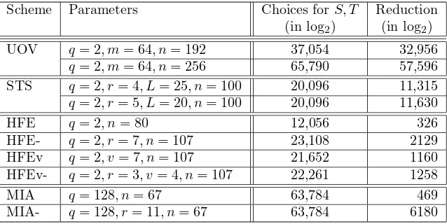
Forq= 2 andn= 80, the number of equivalent keys per private key is≈2326_{. In comparison,} the number of choices forS andT is≈212,056_{. This special choice of parameters has been used in} HFE Challenge 1 [Pat96b].

4.1.1

HFE-We recall that HFE- is the original HFE-class with the minus modification from Section 3.7 applied. In particular, this means that the “shape” of the central polynomialP0_(X0_{) is still the same, i.e.,} all considerations from the previous theorem also apply to HFE-.

Theorem 4.3 ForK := (S, P, T)∈Aff−1(Fn_)×E_[X]×Aff−1₍Fn_{) a private key in HFE and a}

reduction parameterr∈Z+ _{we have}

n.q2n_(qn_−1)(qn−r₋₁₎ n−1

Y

i=n−r−1

(qn_−qi₎

Proof. _{This proof uses the same ideas as the proof of Theorem 4.2 to obtain a normal form of the}

affine transformationS,i.e., applying the additive sustainer, the big sustainer and the Frobenius sustainer on this side. Hence, we have a reduction byn.qn_(qn_{−1) keys here.}

For the affine transformation T, we also have to take the reduction sustainer into account: we use ˜T(X) : Fn _→ Fn−r _{and fix ˜T(0) = 0 by applying the additive sustainer and ˜T(1) =}

1 by applying the big sustainer, which gives us qn−r _{and q}n−r _{−1 choices, respectively. To}

avoid double counting with the reduction sustainer, all computations were performed in ˜E _:=

GF(qn−r_{) rather thanE. Again, we can compute a normal form for a given private key and reverse}

these computations to obtain the full equivalence class for any given private key in normal form. Moreover, we observe that the resulting transformation ˜T allows forqrQn−1

i=n−r−1(qn−qi) choices for the original transformationT :Fn_→Fn _{without affecting the output of ˜T and hence, keeping}

the two fix points ˜T(0) = 0 and ˜T(1) = 1. Therefore, there are a total ofqn−r_·qr_·(qn−r_−1)·

Qn−1

i=n−r−1(q

n_−qi_{) possibilities for the transformationT without changing the public key equations.}

Multiplying out the intermediate results forS andT yields the theorem. ¤

Forq= 2, r= 7 andn= 107, the number of equivalent keys for each private key is≈22129_{. In} comparison, the number of choices forS andT is≈223,108_{. This special choice of parameters has} been used in Quartz-7m [WP04].

4.1.2 HFEv

Another important variation of Hidden Field Equations is HFEv. In particular, it was used in the signature scheme Quartz [CGP01]. HFEv was introduced in [KPG99]. The HFEv scheme is characterized in the following definition.

Definition 4.4 _Let E _{be a finite field with degree n}0 _{over F, v ∈ Z}+ _{the number of vinegar} variables, and P(X) a polynomial overE_{. Moreover, let (z1, . . . , zv) :=sn−v+1(x1, . . . , xn), . . . ,}

sn(x1, . . . , xn)forsithe polynomials ofS(x)in multivariate representation andX0:=φ−1(x01, . . . , x0n0), using the canonical bijectionφ−1_:Fn _→Eandx0

i:=si(x1, . . . , xn)for1≤i≤n0 as hidden

vari-ables. Then define the central equation as

P0

z0

1,...,z0v(X

0_{) :=} X

0≤i,j≤d qi_+qj_≤d

Ci,jX0q i_+qj

+ X

0≤k≤d qk_≤d

Bk(z1, . . . , zv)X0q k

+A0_(z0

1, . . . , zv0)

where

       

      

C0

i,jX0q i_+qj

forC0

i,j∈Eare the

quadratic terms,

B0

k(z10, . . . , zv0)X0q k

forB0

k(z10, . . . , zv0) depending

linearly on z0

1, . . . , z0v and

A0_(z0

1, . . . , zv0) forA0(z10, . . . , zv0)depending

quadratically onz0 1, . . . , zv0

and a degreed∈Z+_{, we say the central equationsP}0 _{are in HFEv-shape.} The condition that theB0

k(z10, . . . , z0v) are affine functions (i.e., of degree 1 in thezi0 at most) and

A0_(z0

1, . . . , z0v) is a quadratic function overFensures that the public key is still quadratic over F.

Theorem 4.5 For K := (S, P0_{, T) ∈ Aff}−1_(Fn_)×E[X0_]×Aff−1_(Fm_{) a private key in HFEv,}

v∈Z+_{the number of vinegar variables,}E_ann0_{-dimensional extension ofFwheren}0_:=n−v=m we have

n0qn+n0+vm(qn0−1)2

v−1

Y

i=0

(qv−qi)

equivalent keys. Hence, the key-space of HFEv can be reduced by this number.

Proof. _{In contrast to HFE-, the difficulty now lies in the computation of a normal form for the}

affine transformationS rather than the affine transformationT. For the latter, we can still apply the big sustainer and the additive sustainer and obtain a total ofqm_·(qm_{−1) =q}n0

·(qn0 −1) equivalent keys for a given transformationT. Moreover, the HFEv modification does not change the “absorbing behaviour” of the central polynomialP0 _{and hence, the proof from Theorem 4.2 is} still applicable.

This reduces the key-space by qn_{. In order to make sure that we do not count the same linear}

transformation twice, we consider a normal form for the now (linear) transformationS

µ

Em Fvm

0 Iv

¶

withEm∈Fm×m, Fvm∈Fm×v.

In the above definition, we also haveIvthe identity matrix inFv×v. Moreover, the left-lower corner

is the all-zero matrix inFv×m_{. The reason for this non-symmetry: we may not introduce vinegar}

variables in the set of oil variables, but due to the form of the vinegar equations, we can introduce oil variables in the set of vinegar variables. This is done by the following matrix. In particular, for each invertible matrixMS, we have a unique matrix

µ

Im 0

Gv m Hv

¶

with an invertible matrixHv∈Fv×v.

which transfers MS to the normal form from above. Again, Im is an identity matrix in Fm×m.

Moreover, we have some matrix Gv

m∈Fv×m. This way, we obtain qvm

Qv−1

i=0(q

v_−qi_{) equivalent}

keys in the “v” modification alone. As stated previously, the identity matrixImensures that the

input of the HFE component is unaltered. However, we do not have such a restriction on the input of the vinegar part and can hence introduce the two matricesGv

m and Hv: they are “absorbed”

into the random terms of the vinegar polynomialsB0

k(z10, . . . , zv0) andA0(z10, . . . , zv0).

For the HFE component overE_{, we can now apply the big sustainer toS and obtain a factor}

of (qn0

−1). In addition, we apply the Frobenius sustainer to the HFE component, which yields an additional factor ofn0_{. Note that the Frobenius sustainer can be applied both toS andT, and} hence, we can make sure that it cancels out and does not affect the degree of the central polynomial

Pz1,...,zv(X). Again, we can reverse all computations and therefore obtain equivalence classes of

equal size for each given private key in normal form. ¤

For the caseq= 2, v= 7 andn= 107, the number of equivalent keys for each private is≈21160_. In comparison, the number of choices forS andT is≈221,652_.

4.1.3

HFEv-Here, we combine both the HFEv and the HFE- modification to obtain HFEv-. In fact, the original Quartz scheme [CGP01] was of this type.

Theorem 4.6 For K := (S, P0_{, T) ∈ Aff}−1_(Fn_)×E[X0_]×Aff−1_(Fm+v_,Fm+r_{) a private key in}

HFEv-,v∈Z+_{vinegar variables, a reduction parameterr∈}Z+ _andE_ann0_{-dimensional extension} ofF _wheren0_{:=n−v andn}0 _{=m+rwe have}

n0_qr+2n0_+vn0 (qn0

−1)2

v−1

Y

i=0

(qv_−qi₎ n0₋₁

Y

i=n0−r−1 (qn0

−qi₎

equivalent keys. Hence, the key-space of HFEv- can be reduced by this number.

Proof. _{This proof is a combination of the two cases HFEv and HFE-. Given that the difficulty}

for the HFE- modification was in the T-transformation while the difficulty of HFEv was in the

S-transformation, we can safely combine the known sustainers without any double-counting. ¤

For the caseq= 2, r= 3, v= 4 andn= 107, n0_{= 103, the number of redundant keys is≈2}1258_. In comparison, the number of choices forS andT is ≈222,261_{. This special choice of parameters} has been used in the original version of Quartz [CGP01], as submitted to NESSIE [NES].

4.2

Matsumoto-Imai Scheme A

As HFE, the MIA class uses a finite fieldF _{and an extension field} E_{. However, the choice of the}

central equation is far more restrictive than in HFE as we only have one monomial here.

Definition 4.7 _Let E_{be an extension field of dimensionnover the finite field}F_{with even}

char-acteristic and λ ∈ Z+ _{an integer with gcd(q}n _{−1, q}λ_{+ 1) = 1. We then say that the following}

central equation is of MIA-shape:

The restriction gcd(qn_{−1, q}λ_{+ 1) = 1 is necessary first to obtain a permutation polynomial and}

second to allow efficient inversion ofP0_(X0_{). In this setting, we cannot apply the additive sustainer} as this monomial does not allow any linear or constant terms. Moreover, the monomial requires a factor of one. Hence, we have to preserve this property. As we will see in Section 5, the only sustainers suitable here are the big sustainer, see Section 3.2, and the Frobenius sustainer from Section 3.6.

Remark. In the paper [MI88], MIA was introduced under the name C∗_{. Moreover, it used the} branching modifier [WP05c, 4.4] by default. As branching has been attacked very successfully, C∗ _{has been used without this modification for any later construction, e.g., [CGP00b, CGP02,} CGP00a, CGP03]. However, without the branching condition, the “new” scheme C∗_{coincides with} the previously suggested “Scheme A” from [IM85]. To acknowledge this historical development, we decided to come back to the earlier notation and call the scheme presented in this section “MIA” for “Matsumoto-Imai Scheme A”. This has been previously suggested in [WP05c].

Theorem 4.8 ForK:= (S, P0_{, T)∈Aff}−1_(Fn_)×E[X0_]×Aff−1_(Fn_{)a private key in MIA we have}

n(qn−1)

equivalent keys. Hence, the key-space of MIA can be reduced by this number.

Proof. _{To prove this statement, we consider normal forms of keys in MIA. In particular, we}

concentrate on a normal form of the affine transformationSwhereSis in univariate representation. As for HFE and w.l.o.g., letB :=S(1) be a non-zero coefficient on Input 1. Unlike HFE we cannot enforce thatS(0) = 0, so we may haveS(1) = 0. However, in this case setB :=S(0). Applying

σ−1_{(X) :=B}−1_{X will ensure a normal form forS. In order to “repair” the monomial P}0_(X0_{), we} have to apply an inverse transformation toT. So letτ(X) := (Bqλ₊₁

)−1_{X. This way we obtain} P = T◦τ−1◦τ◦P0◦σ◦σ−1◦S

= T˜◦(B(qλ+1).(−1)_.Bqλ+1_.X0qλ+1_)◦S˜ = T˜◦P0_{◦S ,˜}

where ˜Sis in normal form. In contrast to HFE in Theorem 4.2, we cannot chose the transformations

σand τ independently: each choice of σ implies a particularτ and vice versa. However, the fix point 1 is still preserved by the Frobenius sustainer and so we can apply this sustainer to the transformation S. As for HFE, we compute a normal form for a given generator and a total ordering ofE_{; again, we “repair” the monomialX}0qλ+1_{by applying an inverse Frobenius sustainer} toT and hence have

(BXqc_{, B}−qλ−1_Xqn−c

)•(S, P0_{, T) whereB ∈E}∗ _{and 0≤c < nforc∈N,}

which leads to a total ofn·(qn_{−1) equivalent keys for any given private key. Since all these keys}

form equivalence classes of equal size, we reduced the private key space of MIA by this factor. ¤

We want to point out that there is also a variation of MIA defined overodd characteristic. This variation has been suggested in [WP05c, Sect. 7.1] and uses exactly the same structure for the private key. For technical reasons, the condition on the gcd is replaced by gcd(qn_{−1, q}λ_{+ 1) = 2.}

However, this is irrelevant for our purpose and we have hence the following corollary.

Corollary 4.9 For K := (S, P0_{, T) ∈ Aff}−1_(Fn_)×E[X0_]×Aff−1_(Fn_{) a private key in MIO we}

have

n(qn−1)

equivalent keys. Hence, the key-space of MIO can be reduced by this number.

The above corollary can be proved in exactly the same way as Theorem 4.8. In particular, the fact that MIO is defined over odd rather than even characteristic does not impose a restriction in this context.

Remark. Patarin observed that it is possible to derive equivalent keys by changing the monomial

P0 _{[Pat96a]. As the aim of this article is the study of equivalent keys by chaining the affine} transformationsS, T alone, we did not make use of this property. A weaker version of the above theorem can be found in [WP05b]; in particular, it does not take the MIO class into account.

Moreover, we observed in this section that it is not possible for MIA to change the transforma-tionsS, T from affine to linear. But Geiselmannet al.showed how to reveal the constant parts of these transformations [GSB01]. Hence, having S, T affine instead of linear does not enhance the overall security of MIA.

4.2.1

MIA-We want to point out that MIA itself is insecure, due to a very efficient attack by Patarin [Pat95]. However, for well-chosen parametersq, r, its variation MIA- (also known as C∗−−_{) is believed to} be secure: as in the case of HFE and HFE-, we use the original MIA scheme and apply the minus modification from Section 3.7.

Theorem 4.10 ForK:= (S, P, T)∈Aff−1_(Fn_)×E[X]×Aff−1_(Fn_{)a private key in MIA and a}

reduction numberr∈Z+ _{we have}

n.(qn_−1)qr n−1

Y

i=n−r−1

(qn_−qi₎

equivalent keys. Hence, the key-space of MIA- can be reduced by this number.

Proof. _{This proof is similar to the one of MIA, i.e., we apply both the Frobenius and the big}

sustainer to S and the corresponding inverse sustainer to the transformation T. This way, we “repair” the change on the central monomialXqλ₊₁

. All in all, we obtain a factor of n·(qn₋₁₎

equivalent keys for a given private key.

Next we observe that the reduction sustainer applied to the transformation T alone allows us to change the last r rows of the vectorvT ∈Fn and also the lastrrows of the matrixMT ∈Fn×n.

This yields an additional factor ofqrQn−1

i=n−r−1(qn−qi) on this side.

Note that the changes on the side of the transformation S and the changes on the side of the transformation T are independent: the first computes a normal form for S while the second computes a normal form onT. Hence, we may multiply both factors to obtain the overall number

of independent keys. ¤

For q = 128, r = 11 and n = 67, we obtain ≈ 26180 _{equivalent private keys per class. The} number of choices forS, T is≈263,784 _{in this case. This particular choice of parameters has been} used in Sflashv3 _[CGP03].

4.3

Unbalanced Oil and Vinegar Schemes

In contrast to the two schemes before, we now consider a class of MQ-schemes which does not mix operations over two different fieldsE_and F_{but only performs computations over the ground}

fieldF_{. Moreover, Unbalanced Oil and Vinegar schemes (UOV) omit the affine transformation T}

but useS ∈Aff−1_(Fn_{). To fit in our framework, we set it to be the identity transformation,i.e.,}

we haveT :=τ:=id. UOV were proposed in [KPG99].

Definition 4.11 _LetF_{be a finite field andn, m∈}Z+_{withn≥2m. Moreover, letα}0

i, βi,j0 , γi,j,k0 ∈ F_{. We say that the polynomials below are central equations in UOV-shape:}

p0

i(x

0

1, . . . , x0n) := m

X

j=1

n

X

k=1

γ0

i,j,kx

0

jx

0

k+ n

X

j=1

β0

i,jx

0

j+α

0

i.

In this context, the variables x0

i for 1 ≤ i ≤ m are called the “vinegar” variables and x0i for

m < i≤n the “oil” variables. Note that the vinegar variables are combined quadratically while the oil variables are only combined with vinegar variables in a quadratic way. Therefore, assigning random values to the vinegar variables, results in a system of linear equations in the oil variables which can than be solved, e.g., using Gaussian elimination. So the “shape” of UOV is the fact that a system in the oil variables alone is linear. Hence, we may not mix oil variables and vinegar variables in our analysis but may perform affine transformations within one set of these variables. So for UOV, we can apply the additive sustainer and also the Gauss sustainer, introduced in sections 3.1 and 3.5. However, in order to ensure that the shape of the central equations does not change, we have to ensure that the Gauss sustainer influences the vinegar and oil variables separately.

Theorem 4.12 LetK:= (S,P0_,id)∈Aff−1_(Fn_{)× MQ(F}n_,Fm_)×Aff−1_(Fm_{)be a private key in}

UOV. Then we have

qn+mn n−m−1

Y

i=0

(qn−m_−qi₎ m−1

Y

i=0

(qm_−qi₎

Proof. _{As in the case of the schemes before, we compute a normal form for a given private key.}

First, applying the additive sustainer reduces the affine transformationSto a linear transformation. This results in a factor ofqn _{in terms of equivalent keys. Second, applying the Gauss sustainer}

separately within vinegar and oil variables, we can enforce the following structure, denotedR ∈

Fn×n_{, on the matrixMS ∈}Fn×n _{of the (now only) linear transformation S:}

R:=





Im 0 Am

0 In−2m Bmn−2m

0 0 Im



 .

In this context, the matricesIm, In−2m are the identity elements of Fm×m and F(n−2m)×(n−2m),

respectively. Moreover, we have the matricesAm∈Fm×m andBmn−2m∈F(n−2m)×m. For a given

central equationP0_{, each possible matrixR leads to the same number of equivalent keys. Let}

E:=

µ

Fn−m 0

Gm

n−m Hm

¶

be an (n×n)-matrix. Here, we require that the matricesFn−m∈F(n−m)×(n−m)andHm∈Fm×m

are invertible and hence the counting from Lemma 2.4 applies. ForGm

n−m∈Fm×(n−m), we have

no restrictions. This way, we define the transformationσ(x) :=Exwherex∈Fn_{. Note that these}

transformationsσform a subgroup within the affine transformations. So we have

(Ex+a,id)•(S,P0_{,id) fora∈F}n _{andE as defined above.}

As this choice ofσpartitions the private key space into equivalence classes of equal size, and due to the restrictions onE, we reduced the size of the private key space by an additional factor of

qmnQn−m−1

i=0 (q

n−m_−qi₎Qm−1

i=0 (q

m_−qi_).

¤

For q = 2, m = 64, n = 192, we obtain 232,956 _{equivalent keys per key — in comparison to} 237,054 _{choices for S. If we increase the number of variables to n = 256, we obtain 2}57,596 _and 265,790_{, respectively. Both choices of parameter have been used in [KPG03].}

4.4

Stepwise-Triangular Systems

Unbalanced Oil and Vinegar schemes and Stepwise-Triangular Systems (STS) are quite similar as both are defined over small ground fields rather than ground fields and extension fields. In addition, they enforce a special structure on the input variables. In the case of UOV we have two sets of variables while we useL∈Z+_{such sets in the case of STS, each forming onelayer orstep.}

These layers form a generalized triangular structure, hence the name of these schemes. We capture this intuition more formally below. Stepwise Triangular Schemes were introduced in [WBP04].

Definition 4.13 _{Let n1, . . . , nL ∈}Z+ _{be L integers such thatn1+· · ·+nL =n, the number of}

variables, and m1, . . . , mL∈Z+ such that m1+· · ·+mL=m, the number of equations. Herenl

represents the number of new variables (step-width) andml the number of equations (step-height),

both in Step l for 1≤l ≤L. By convention, we set n0 :=m0 := 0. Now let P0 ∈ MQ(Fn,Fm) be a system ofMultivariateQuadratic polynomials such that theml private quadratic polynomials

p0

m0+...+ml−1+1, . . . , p 0

ml of each layer l contain only the variables x

0

k with k ≤

Pl

j=1nj, i.e.,

only the variables defined in all previous steps plus nl new ones. Then we call (S,P0, T,) ∈

Aff−1(Fn_{)× MQ(}Fn_,Fm_)×Aff−1₍Fm_{) a private key in Stepwise Triangular System shape. If}

n1=. . .=nL=m1=. . .=mL=r for somer∈Z+, we call this a regularStepwise Triangular

System.

We want to stress in this context that we do not assume any additional structure for the private polynomialsp0

1, . . . , p0mhere. In particular, all coefficientsγi,j,k0 , β

0

i,j, α0i ∈F for these polynomials

may be chosen at random.

As STS and UOV are based on a similar concept, the following proof on Stepwise Triangular Schemes uses the same ideas as the proof for the UOV class. As for UOV we exploit the fact that we can use Gauss operations within any given layer — and use again the fact that equations of Layer l depend on all variables of the layers 1, . . . , l, i.e., we may also perform Gauss operations on these previous layers, as long as the result only affects the given Layerl.

Theorem 4.14 Let F _{be a finite field with q := |}F_{| elements, n ∈} Z+ _{the number of variables,}

(Z+₎L _{be a vector of integers such thatn1+. . .+nL=nandm1, . . . , mL∈}Z+ _{integers such that}

m1+. . .+mL=m. Then forK:= (S,P0, T)∈Aff−1(Fn)× MQ(Fn,Fm)×Aff−1(Fm)a private

key in STS we have

qm+n L

Y

i=1



q

ni(n−Pij=1nj)

ni−1

Y

j=0

(qni_−qj₎

  L Y i=1  q

mi(m−Pij=1mj)

mi−1

Y

j=0

(qmi_−qj₎





equivalent keys. Hence, the key-space of STS can be reduced by this number.

Proof. _{For this proof, we apply both the additive sustainer and the Gauss sustainer. The latter}

is applied independently on each layer.

First, we observe that we can apply the additive sustainer both to the transformation S ∈ Aff−1(Fn_{) andT ∈Aff}−1₍Fm_{) to obtain the fix point S(0) =T(0) = 0. As a result, we obtain a}

factor of qm+n _{and may assume S ∈Hom}−1_(Fn_{) and T ∈Hom}−1_(Fm_{) for the remainder of this}

proof.

As in the proof of Theorem 4.12, we impose a special structure on the linear transformation S. Therefore, we consider the matrix

MS :=

              

In1 ∗ ∗ · · · ∗ ∗

0 In2 ∗ ∗

0 0 In3

..

. . .. ...

InL−2 ∗ ∗

0 0 InL−1 ∗

0 0 · · · 0 0 InL

              

In MS ∈ Fn×n, sub-matrices Ini are identity matrices in F

ni×ni _{for 1 ≤i ≤ n. The left lower}

portion ofMS is zero while the upper right portion ofMS consists of elements ofF. To obtain this

matrixMS, we make use of

E :=               

An1 0 0 · · · 0 0

∗ An2 0 0

∗ ∗ An3

..

. . .. ...

AnL−2 0 0

∗ ∗ AnL−1 0

∗ ∗ · · · ∗ ∗ AnL

              

In this matrixE ∈Fn×n_{, we have invertible componentsAni ∈}Fni×ni _{for 1≤i≤L. Moreover,}

the upper right portion of the matrixEis zero while the left lower portion ofEconsists of elements ofF_{. We see that the above matrix is sufficient to impose this special structure onMS. Moreover,}

for each choice ofE, we obtain another linear transformationS and hence,MS is a normal form

ofS.

Using Lemma 2.4, we can now count the number of possible matricesE and obtain

L

Y

i=1



q

ni(n−Pij=1nj) ni−1

Y

j=0

(qni_−qj₎





for the number of possibilities. To see the correctness of the above computation, we specialise it forn1: here we have the termQnj=01−1(qn1−q

j

) which computes the number of choices for the matrix

An1 while q

n1(n−n1) _{gives the number of choices in the (n}

1×(n−n1)) column overF below the matrixAn1. By induction onniwe obtain the above formula for 1≤i≤L. In particular, asMSis in normal form, there exists exactly one matrixEof the above form for any givenS ∈Hom−1_(Fn_).

Hence, we have established the existence of an equivalence class of this size.

The corresponding proof for the transformationT is analogous, so we can define matrixE0_∈

different roles the transformations S and T play. Note that we are allowed to add equations of lower layers to equations of higher layers and hence, may perform the same Gauss operations on equations that we could apply on variables. So we have

(Ex+a, E0_x+a0_)•(S,P0_{, T) fora∈F}n

, a0_∈Fm

andE, E0 _{defined as above.}

As this choice ofσ, τ partitions the private key space into equivalence classes of equal size, and due to the restrictions onE, E0_{, we reduced the size of the private key space by the above number. ¤}

Corollary 4.15 For regular STS with step-width r ∈Z+_{,L ∈}Z+ _{layers and n:=Lr variables,}

the above formula simplifies to

q2n

Ã_L Y

l=1

qr(n−(l−1)r)

r−1

Y

i=0

(qr−qi)L

!2

.

Choosing a regular STS scheme andq= 2, r= 4, L= 25, n= 100, we obtain 211,315_equivalent keys for each given private key. For comparison: the number of choices for the two affine transfor-mationsS, T is 220,096_{. Changing the number of layers to 20, and consequently having r= 5, we} obtain a total of 211,630 _{equivalent keys. These special choices of parameters have been suggested} in [KS04].

5

Tightness for MIA and MIO

All theorems in the previous section suffer from the same problem: we do not know if the size-reductions are “tight”,i.e., if the sustainers applied are the only ones possible. In this section we proof that for the MIA/MIO class, the big sustainer and the Frobenius sustainer are actually the only possible way to achieve equivalent keys for MIA and MIO. We recall that both classes use a finite field F _{with q := |}F_{| elements and an extension field} E _{of dimension n over} F_{. Over} E_,

they use the monomial Y0 _{:= X}0qλ₊₁

as central equation for 1 ≤λ < n. While MIA needs q to be even, MIO is defined forq being odd. The proof for the MIA case is based on an unpublished observation by Dobbertin. Its extension to the MIO class is due to the authors.

The starting point of the proof is the following equation which needs to hold for any two equivalent keys for the MIA / MIO class. This is due to the fact that Definition 2.1 restricts us to affine transformations to transfer one private key into. Hence we have the following equation:

Xqλ₊₁

=T◦Xqλ₊₁

◦S ,

which we can rewrite as

Xqλ+1◦S−1_=T◦Xqλ₊₁

. (2)

We know from Section 2.1 that affine transformations form a group. Moreover, we can use Defi-nition 2.7 to obtain a univariate representation for any given affine transformation. We can hence express (2) as

Ã_n−1 X

i=0

BiXq i

+A

!qλ+1

=

n−1

X

i=0 ˜

Bi

³

Xqλ₊₁´qi

+ ˜A ,

for some coefficientsA,A, B˜ i,B˜i ∈E. Note that we have (A+B)p =Ap+Bp in a finite field of

characteristicpand consequently (A+B)q _=Aq_+Bq _forq=pk_{and somek∈Z}+_{. We now use a} matrix representation of the above equation, similar to the matrix used by Kipnis and Shamir in their cryptanalysis of HFE [KS99]. This yields

      

Aqλ+1 _ABqλ

0 Xq

λ

ABqλ+1

1 Xq

λ+1

. . . ABqλ+n−1 n−1 X

qλ+n−1

B0Aq

λ

X Bqλ+1

0 Xq

λ₊₁

B0Bq

λ

1 Xq

λ+1₊₁

B0Bq

λ

n−1X

qλ+n−1+1

B1Aq

λ

Xq _B

1Bq

λ

0 Xq

λ₊

q _Bqλ+1

1 Xq

λ+1₊

q _{. . . B}

1Bq

λ

n−1X

qλ+n−1+q

. . . . . . . .. ...

Bn−1A

qλ_Xqn−1_B n−1B

qλ

0 Xq

λ₊

qn−1_B n−1B

qλ

1 Xq

λ+1₊

qn−1_{. . . B}qλ+1 n−1 X

qλ+n−1+qn−1        =        ˜

A 0 . . . 0

0 B˜qλ+1

0 Xq

λ₊₁

0 0

0 B˜qλ+1+q

1 Xq

λ+1₊

q ₀

. .

. . .. ...

0 0 0 . . . B˜qλ+(n−1)+qn−1

n−1 X

As we work inE _{which has a multiplicative group ofq}n_{−1 elements, we can reduce all powers}

larger than or equal toqn _byqn_−1.

Lemma 5.1 ForF _{a finite field withq > 2 elements, we can only use the big sustainer and the}

Frobenius sustainer to derive equivalent private keys within the MIA and the MIO class.

Proof. _{For this proof we show that the equations given by (∗) imply thatA= 0 and allBi for}

0≤n < nexcept one are zero. Note thatB0=. . .=Bn−1= 0 implies thatS(X) is no bijection anymore but the transformation S(X) =A for any inputX ∈E _{and fixedA ∈}E_{. Hence, there}

must exist at least one non-zero coefficientBi. W.l.o.g., we assume thatB0 is non-zero. Note that this lemma is trivially true for an extension field of degreen= 1. Hence, we assume thatE _{is a}

proper extension ofF _{and thereforen≥2.}

For the proof, we make use of the fact that we can reduce all powers in E _{by q}n _{−1. For}

powers of the formqi _{this means that we can reduce the poweri byn,i.e., all computations are}

done in the ringZ_/nZ_{and we can hence assume 0≤a, b, c, d < nin the sequel. Moreover, we can}

distinguish the following three types of equations in (∗):

1. Equations of the formABqλ+a_+Bqb b A

qλ _{= 0 fora+λ≡b (mod n). We call themequations}

of type A. Note that they are related to terms with monomial of the formXqb _{for 0≤b < n.}

2. Equations of the formBqλ+a

a B

qb

b = 0 with the conditiona+λ≡b (mod n) on the powers.

We call themequations of Hamming weight 1 and say that they areself-dual. Note that each row / column in the above matrix contains exactly one equation of Hamming weight 1 and that they correspond to terms with a monomial of the formX2qb

for 0≤b > n. As we have

q >2 there is no reduction of the power here.

3. Equations of the form Bqλ+a

a B

qb b +B

qλ+c

c B

qd

d = 0 with the following conditions on their

powers: first, we have a 6= b, c 6= d, as we otherwise would include equations from the diagonal. Obviously, we cannot make the assumption anymore that the right-hand side is equal to zero in this case. Second, we havea+λ6≡b (modn) andc+λ6≡d (modn) as we obtain equations of Hamming weight 1 otherwise. Third, we needa+λ ≡d (modn) and

c+λ≡b (modn) to ensure that the powers in the monomial Xqb_+qd

actually match. We call the pair (a, b) thedual of the pair (c, d). Note that this relation is reflexive,i.e., (c, d) is the dual of (a, b). We call theseequations of type B.

Note that equations of type A and equations of Hamming weight 1 do not mix as we haveq >2. Moreover, equations of Hamming weight 1 may not lie on the diagonal as we would haveλ+a≡a

(modn) in this case and hence λ≡0 (modn), but this violates 0 < λ < n. So far, we did not include any equation from the diagonal in our analysis. We come back to them later.

Inspecting the equation B0qλB

qλ

λ = 0 of Hamming weight 1, we see that it impliesBλ = 0 as

we haveB06= 0 (see above). In addition, this implies A= 0 as we haveABq

λ

0 +B

qλ λ A

qλ

= 0 as an equation of type A. Forn= 2, we are done. For n≥3, we can now use all equations of type B of the formBq0λB

qb b +B

qλ+c

c B

qλ

λ = 0. We notice that we need to meet the following conditions:

b6= 0, λ and c 6= 0, λ but c+λ≡b (mod n). We see that we can construct pairs (b, c) meeting this conditions for all b ∈ Z_/nZ_{\{0, λ,2λ} with 0 < b < n. Using the above equation we have}

established that all coefficients Bb = 0 asB06= 0 and Bλ= 0. Note that λ6≡2λ (modn) as we

have 0< λ < n. Moreover, 2λ6≡ 0 (modn) is not true either, which we see with the following argument: due to the size condition onλ, we know that we need to have 2λ=nto make the above equation hold. We use the condition gcd(qn_−1qλ_{+ 1) = 1 for MIA and gcd(q}n_−1qλ_{+ 1) = 2 for}

MIO to show that 2λ=n is impossible. Therefore we observe that (q2λ_{−1) = (q}λ_{+ 1)(q}λ_−1),

i.e., the gcd condition is violated for n= 2λ.

All left to show is that the coefficientB2λis also equal to zero. To this end, we use the equation

B₂qλ3λB q0 0 +B

q0 −λB

q3λ

3λ = 0 of type B. In order to force the coefficient B2λ equal to zero, we need

B−λ = 0 orB3λ= 0. Therefore, we use the equationB−λq0B0q0= 0 of type Hamming weight 1. As we haveB06= 0, this impliesB−λ and henceB2λ= 0.

We have now established that all coefficientsA=B1=. . .=Bn−1= 0. Using the equations on the diagonal, these conditions also propagate through to the coefficients of the affine transformation

T,i.e., to ˜A,B˜afor 0< a < n. Given that all coefficients butB0are zero, all equations which have terms of the formBaBb fora6= 0, b6= 0 on the left hand side are now also zero, i.e., they do not

influence the equations of the formBiqλ+iB qi i = ˜B

qλ+j j B˜

qj

j for somei, j with 0≤i, j < n. We can