Using Multi-Class Machine Learning Methods to Predict Major League Baseball Pitches.

(1)

ABSTRACT

SIDLE, GLENN DANIEL. Using Multi-Class Machine Learning Methods to Predict Major League Baseball Pitches. (Under the direction of Hien Tran.)

As the field of machine learning and its applications grow, there is a need to expand the ability to classify and predict beyond just being able to handle a binary problem. While the ability to predict a yes or no answer is still valuable, in a world of increasing complexity, machine learning methods are now employed in a multi-class problem setting more than ever.

Major League Baseball provides a rich and detailed data set with its PITCHf/x system that tracks every baseball pitch thrown in every stadium in every game. Pitch prediction has been a topic of previous research that has mostly focused on the binary split between fastballs and other pitch types. We extend the binary problem to a multi-class one that involves up to seven unique pitch types. The work done with baseball pitches can be used as a template to expand a wide variety of other binary predictions into accommodating more than a simple two class approach. To accomplish the multi-class prediction, we examine multiple machine learning methods to find the most efficient and accurate algorithm.

(2)

(3)

Using Multi-Class Machine Learning Methods to Predict Major League Baseball Pitches

by

Glenn Daniel Sidle

A dissertation submitted to the Graduate Faculty of North Carolina State University

in partial fulfillment of the requirements for the Degree of

Doctor of Philosophy

Applied Mathematics

Raleigh, North Carolina

2017

APPROVED BY:

John Griggs Negash Medhin

Kevin Flores Hien Tran

(4)

DEDICATION

(5)

BIOGRAPHY

(6)

ACKNOWLEDGEMENTS

I would like to thank my advisor, Dr. Hien Tran, for all the help and guidance he has given over the past four years, as well as his willingness to let me spend years working on sports analytics research. Also, I want to thank Dr. John David, who was the first person to ever introduce me to the world of machine learning and who encouraged me to pursue topics that I was passionate about. And I will always be grateful to Dr. Stacey Levine, my advisor at Duquesne, who sparked my passion for research and problem solving.

I would like to thank my parents, my brothers, my aunt and uncle, and the rest of my family for their support and the motivation to research something that I can explain at Thanksgiving. I am, and always will be, indebted to my friends for their round-the-clock help, advice, and availability whenever I need them.

(7)

TABLE OF CONTENTS

LIST OF TABLES . . . vii

LIST OF FIGURES. . . .viii

Chapter 1 INTRODUCTION . . . 1

1.1 Prior Work . . . 2

1.2 Overview and Contributions . . . 4

Chapter 2 Feature Selection . . . 5

2.1 PITCHf/x . . . 5

2.2 Training and Testing Sets . . . 7

2.3 Input Features . . . 7

2.3.1 Expert Feature Selection . . . 9

2.4 Contributions . . . 11

Chapter 3 METHODS . . . 12

3.1 Linear Discriminant Analysis . . . 13

3.1.1 Fisher’s Linear Discriminant . . . 13

3.1.2 Binary Classificiation . . . 14

3.1.3 Multi-Class Classification . . . 16

3.2 Support Vector Machines . . . 17

3.2.1 Linearly Separable Case . . . 17

3.2.2 Nonseparable Case . . . 20

3.2.3 Kernel Function . . . 23

3.2.4 Multi-Class SVM . . . 25

3.3 Classification Trees . . . 26

3.3.1 Random Forests . . . 28

3.4 DIRECT Algorithm . . . 29

3.5 Committee Approach . . . 31

Chapter 4 PREDICTION RESULTS. . . 35

4.1 Comparison of Methods . . . 36

4.2 Results Analysis . . . 37

4.2.1 Results by Type of Pitcher . . . 37

4.2.2 Individual Results . . . 38

4.2.3 Results by Count . . . 40

4.2.4 Correlation with Standard Statistics . . . 41

Chapter 5 DDAGs AND FEATURE ANALYSIS . . . 44

(8)

5.2.1 F-Scores . . . 47

5.2.2 ROC Curves . . . 48

5.2.3 Reduced Subset Results . . . 50

5.3 Variable Importance . . . 53

Chapter 6 LIVE IMPLEMENTATION . . . 58

6.1 Conversion to Python . . . 59

6.1.1 Live Prediction Limitations . . . 63

6.2 iOS App Development . . . 63

Chapter 7 CONCLUSION AND FUTURE WORK . . . 67

7.1 Summary of Contributions . . . 67

7.2 Pitch Prediction Future Work . . . 68

BIBLIOGRAPHY . . . 70

APPENDIX . . . 74

(9)

LIST OF TABLES

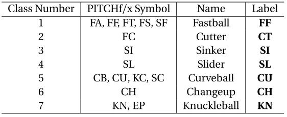
Table 2.1 The different types of pitches considered. . . 7

Table 2.2 Properties of the training and testing sets for individual pitchers. . . 8

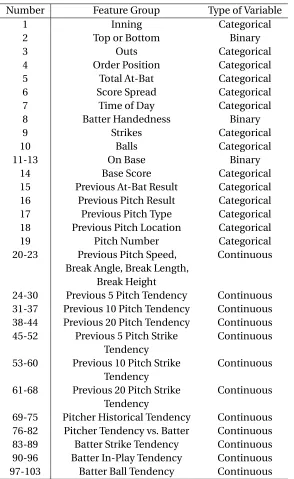
Table 2.3 Feature groups for each pitch. Numbers are given if the pitcher throws all seven pitch types. Tendency refers to the percentage of each pitch type. . . 10

Table 4.1 Average parameters values for all committee members for all pitchers. . . 36

Table 4.2 Comparison of prediction results for each method. . . 37

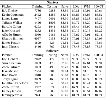
Table 4.3 Comparison of prediction results for starters and relievers. . . 38

Table 4.4 10 highest predicted starters and 10 highest predicted relievers by the random forests, training and testing set sizes, naive guesses, and comparison to LDA and SVM results. . . 39

Table 4.5 100 CTpitch-specific model predictions for Jeremy Guthrie, overall accuracy 37.94%. . . 40

Table 4.6 100 CTpitch-specific model predictions for Odrisamer Despaigne, overall accuracy 53.30%. . . 40

Table 4.7 Average Prediction accuracy for each pitch count for the100 CT method. Pitcher favored counts are shown in bold, batter-favored counts in italics. . . . 41

Table 4.8 Number of pitchers predicted 100% accurate for each count. . . 42

Table 4.9 100 CT Prediction Improvement Compared to FIP and WAR. . . 42

Table 5.1 Average features remaining given different thresholding measures for F-Scores and ROC AUC. . . 50

Table 5.2 Average values comparing different preprocessing techniques for the reduced subset of 282 pitchers. . . 52

Table 5.3 Variable Importance for LDA Delta Predictor and CT Permuted Variable Delta Error for all pitchers. 1 means highest importance, 29 means lowest importance. 55 Table 5.4 Variable Importance for LDA Delta Predictor and CT Permuted Variable Delta Error broken down by starts and relievers. . . 56

Table 6.1 Details of the testing dataset from 9/1/2016 to 10/2/2016 used for the live predictions. . . 60

Table 6.2 Results of the live prediction method for September 1st, 2016 through October 2nd, 2016. . . 62

Table 6.3 Python live pitch predictions for September 1st through October 2nd, 2016, with overall accuracy 58.69%. . . 62

(10)

LIST OF FIGURES

Figure 2.1 A sample at-bat screenshot from the gd2.mlb.com site. . . 6

Figure 2.2 The zones used to determine the location where the pitch crosses home plate. 8 Figure 3.1 Example of a bad (a) and good (b) hyperplanes found for LDA. . . 15

Figure 3.2 An example of a linearly separable binary problem with SVM. . . 17

Figure 3.3 An example of a nonseparable binary problem with SVM. . . 21

Figure 3.4 Example of a kernel function mapping. . . 24

Figure 3.5 A visual representation of the one-vs-all method (thin lines) compared to the one-vs-one method (thick line) from[2]. . . 26

Figure 3.6 Basic Classification Tree for Pitch Selection. . . 27

Figure 3.7 Two sample splits for a decision tree with four unique classes. The split on the left is better, as total impurity is lower due to having higher proportions of fewer classes present in each leaf, minimizing the gdi. Taken from[30]. . . . 28

Figure 3.8 An example initialization of the DIRECT method for two parameter optimiza-tion. . . 30

Figure 3.9 An example of four iterations of the DIRECT algorithm. Possible optimal rectangles are highlighted in yellow for each iteration. . . 31

Figure 3.10 A visual representation of the three reasons why an ensemble method works better than a single one, taken from[15]. Each committee member is repre-sented in blue, with the true classifier labeled in red. . . 33

Figure 5.1 A DAG visualization for the classification of five pitch types. A binary classifier is trained for each pair of pitch types in the ellipses. . . 46

Figure 5.2 An example of how the DAG classifier labels an unknown input. . . 46

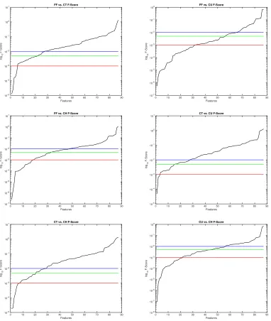
Figure 5.3 Score plots for the six binary splits of pitches thrown by Corey Kluber. F-Scores are shown in log₁₀. Thresholding levels of 0.01, 0.005, and 0.001 are shown in blue, green, and red, respectively. . . 49

Figure 5.4 Highest two AUCs and lowest two AUCs for Corey Kluber for Fastball vs. Curve-ball split. The highest AUC, 0.8414, for his historical tendency to throw a fastball, is shown in green; the second-highest, 0.7123, for the percent of the last five pitches that were curveballs in blue; the second-lowest, 0.322, for his historical tendency to throw a changeup in magenta, and lowest, 0.1219, for his historical tendency to throw a slider in red. The black line in the middle has an AUC of 0.5. . . 51

Figure 6.1 Example of the Python interface for live pitch prediction on the command line in OSX. . . 61

Figure 6.2 Progression of daily prediction accuracy from September 1st to October 2nd. 63 Figure 6.3 Histogram of error between predicted pitch speed and actual pitch speed. . . 64

Figure 6.4 Histogram overlay between the predicted zones and actual zones. . . 65

(11)

CHAPTER

1 INTRODUCTION

Major League Baseball (MLB) is a massive organization with close to 10 billion dollars in revenue in 2015[10], and is only getting bigger. One of the biggest draws to a baseball game is scoring, and as pitching skill has increased over the past few years, it has become more and more important for a runner to get on base. Of the 31 teams that advanced to the postseason over the past three seasons, 25 of those teams ranked in the top half of the league in on-base-percentage (OBP), and 21 of those were in the top ten teams in OBP[17]. OBP is a measure not only of a batter’s ability to get a hit, but also draw a walk or, in rare cases, get an intentional walk, get hit by a pitch, or have a third strike dropped. As statistical analysis has become more and more common in baseball, OBP is replacing batting average as a true mark of a batter’s ability[31]. Being able to anticipate the next type of pitch that will be thrown would help a batter decide to swing or not, given the tendency of some pitches to result in balls or strikes.

While we employ machine learning in an effort to predict the type of pitch that will be thrown, the initial classification of a pitch is a difficult problem alone. MLB Advanced Media (MLBAM) employs a neural network algorithm that automates this task, and we consider seven unique pitch types as classified by MLBAM.

(12)

pitch, we create individual models for each pitcher. Being able to predict from up to seven different pitch types is not a trivial problem, however, as many machine learning methods were designed originally for binary type prediction. Extending these methods from two classes to more involves an exponential increase in complexity and computation time, as well as being susceptible to large class imbalances. We measure our success not only in overall accuracy but also relative to the best naive guess, as well as the ability of the method to beat the naive guess for the set of pitchers.

1.1 Prior Work

Much of the previous work has focused on a binary split between baseball pitches into the categories of fastball and not fastball. In[23], Guttag et al., looked at 359 pitchers, training the model with data from 2008 and testing with data from 2009 and comparing their models predictive accuracy against a naive guess (which we will discuss in Chapter 4). They achieved an average accuracy of 70%, with varying degrees of success depending on the pitcher’s initial naive guess and amount of available data.

With feature selection, this binary prediction has achieved close to 80% accuracy[27], but has many problems associated with it. There is no unifying definition of a "fastball." While two and four seam fastballs are the most obvious members of the category, pitches such as sliders, sinkers, and cutters can often be included as well, despite having very different appearances and behavior when thrown. Our initial work involved using at least five different types of pitches, but we eventually extended our prediction to incorporate seven pitch classes. Guttag et al., also modified the binary approach to consider other types of pitches against the others, and in doing so addressed up to six different types of pitches: fastballs, changeups, sliders, curveballs, split-finger fastballs, and cutters[23]. To our knowledge no other binary approaches have been modified this way to consider pitch types other than fastballs as the "positive" class.

Bock et al.,[7]is the only publication in a scientific journal that has used a multi-class approach to pitch prediction, predicting up to four unique pitch types. The authors of the paper employed a one-versus-all (which we will discuss more in Chapter 3) support vector machine based method using a linear and radial basis kernel functions. Using a data set of 402 pitchers from the 2011, 2012, and 2013 seasons, they used the cross validation accuracy as a measure of predictability. Across all pitchers, they report an average cross-validation accuracy of 74.5%. The authors then examine the correlation between the predictability of the pitcher and some standard statistics, looking to forecast pitcher success. They examined the ERA and FIP of each pitcher, eventually determining there was "no significant relationship" between predictability and performance.

(13)

of set sample taken only from a subset of pitchers who pitched in the 2013 World Series. Because the focus of the paper was on using predictability to gauge long term pitcher performance, the out of sample accuracy was only briefly mentioned. The authors used a range of 14 pitchers from the World Series who faced as few as five batters and as many as 60, resulting in possibly skewed or class imbalanced datasets. While this out of sample accuracy is a proof of concept, the number of pitchers and size of the datasets used do not give a well-tested measure of the model’s ability to predict pitches it hasn’t seen before.

Another multi-class prediction method was proposed in[53]where the author employed a decision tree based method. This work again only examined four different pitch types and also restricted the results to a proof of concept based on the prediction performance for two pitchers. Woodward discusses the results for Justin Verlander and Clayton Kershaw, stating that overall prediction for Verlander is 50%, well below the naive guess for Verlander. He does, however, examine the performance of the decision tree classifier measured against totally random guessing. Our work incorporates many of the ideas proposed in[7]and[53], but we extend the number of classes and the research to optimize our methods in a much more thorough manner.

While multi-class machine learning methods have not been applied to the problem of pitch prediction outside of[7]and[53], they have been implemented to predict or classify other types of problems. Multi-class support vector machines are used on a number of standard datasets from the UCI machine learning repository in[29]and[51]. Both[29]and[51]are comparison papers, giving an overview of the different formulations of the multi-class support vector machine method, tested on datasets with a minimum of four classes and a maximum of 17 classes.

In[25], the multi-class support vector machine is demonstrated on massively multi-class datasets, i.e., classifying an image of a flower into one of roughly 20,000 types of flowers. While the support vector machine models did not outperform the method the authors were introducing, it is an excel-lent demonstration of the extendability of the support vector machine classification on datasets of up to more than 96,000 classes.

As linear discriminant analysis is not the most common machine learning classification method, even for binary problems, few multi-class journal articles have been published. A survey paper by Li et al.,[32]gives an overview of the method and its extension to multi-class classification, again using many of the same benchmark datasets from the UCI repository as[29]and[51]as well as others. In this paper, linear discriminant analysis is used on datasets ranging from three to one hundred unique classes.

(14)

Holmes et al., introduce alternating decision trees in[28], applying the classifier to binary datasets as well as multi-class datasets also ranging from three to 26 classes. The successes in implementing the different machine learning methods in previous works gives us a good starting point for the pitch prediction problem, where we encounter pitchers with pitch classes ranging from two to seven pitch types.

1.2 Overview and Contributions

In Chapter 2 of this work, we first detail the PITCHf/x system and the data we mined from the repository provided by the MLB. We introduce a novel feature set, including not only observable measurements or historical trends but a combination of the two, balancing the risk of uncertainty and the extra information gained from the PITCHf/x system. Chapter 3 provides an overview of the machine learning methods we use for prediction, our parameter optimization algorithm, and an explanation of the committee approach, which has been very lightly used in previous work for multi-class problems. We also introduce the use of the DIRECT method for parameter optimization for the classifiers we use.

We present our results from each method in Chapter 4 and determine the best method based on accuracy and efficiency, demonstrating better than state of the art results from all the methods exam-ined. As well as presenting the overall results, we also show a breakdown by relievers versus starters and compare our improvement against a naive guess to standard metrics of pitcher performance. In Chapter 5 we detail the decision directed acyclic graph implementation of the multi-class methods. We also employ feature selection in an innovative approach, using the unique architecture of the directed graph implementation to use binary feature selection methods. In the same chapter we also use post-processing methods to measure levels of variable importance and consider whether the results match our expectations.

(15)

CHAPTER

2 FEATURE SELECTION

Baseball is one of the most popular sports in the world and is played in countries around the globe. Because of its unique method of gameplay, baseball is easily broken into discrete events. Each pitch and its subsequent result can be observed and recorded in real time. The MLB is considered to be the highest level of baseball in the world, and as such has some of the most advanced technology available to measure and record different data about each game.

2.1 PITCHf

/

x

(16)

pitcher releases the ball.

In order to download the data, we used the MAMP software stack. MAMP is an open-source software that runs on Apple computers, its name coming from the operating system Mac OSX, the web server Apache, the database management system MySQL, and the programming languages PHP, Perl, and Python[33]. MAMP uses a structured query language (SQL) to scrape data off the .xml pages found on gd2.mlb.com. This data was downloaded to a comma separated value (.csv) file that can be opened in Excel. We used this structured data in MATLAB.

All PITCHf/x data is stored at gd2.mlb.com and available to the public. Figure 2.1 shows what an example at-bat looks like from the .xml version of the data on the site itself (the data is from the last at-bat from the 2016 World Series) with all the individual information provided for each pitch.

Figure 2.1: A sample at-bat screenshot from the gd2.mlb.com site.

We used data from the 2013, 2014, and 2015 regular seasons, which amounted to nearly 2.1 million total unique pitches. We included both starting pitchers, who throw just over 100 pitches per start, making up to 30 or 35 starts per season as well as relievers and closers, who play in many more games but throw fewer pitches per appearance[12]. We restricted our data set only to pitchers who threw at least 500 pitches in both the 2014 and 2015 seasons, which left us with 287 total unique pitchers, 150 starters and 137 relievers as designated by ESPN. Because each pitch that is thrown is classified by MLBAM’s neural network method, each pitch is also assigned a confidence level, and in order to ensure the fidelity of our data we restricted the data to pitches with a type confidence level above 80%. The average size of the data set for each pitcher was 4,682 pitches, with the largest 10,343 pitches and the smallest 1,108 pitches.

(17)

Table 2.1 shows the PITCHf/x label, the common name, and the label we use.

Table 2.1: The different types of pitches considered.

Class Number PITCHf/x Symbol Name Label

1 FA, FF, FT, FS, SF Fastball FF

2 FC Cutter CT

3 SI Sinker SI

4 SL Slider SL

5 CB, CU, KC, SC Curveball CU

6 CH Changeup CH

7 KN, EP Knuckleball KN

2.2 Training and Testing Sets

Most of the authors in previous literature split data into training and testing sets based on different seasons. Our first split of data used all of 2013 and 2014 as the training set for each pitcher and all of 2015 as the testing set. But, because pitchers change their behavior over time[6], we needed to take that into account. During the offseason, pitchers will decide to work on or change pitch types that they use, or develop entirely new pitch types and scrap old ones. To account for the possible changes in pitcher behavior, we decided to include the first quarter of each pitcher’s 2015 season as part of the training set, and use the remainder of the 2015 season as the testing set. Table 2.2 shows the properties of the training and testing sets as well as the amount of pitchers throwing the respective number of pitches in our training and testing sets.

2.3 Input Features

(18)

Table 2.2: Properties of the training and testing sets for individual pitchers.

Value Training Set Testing Set

Average Size 3,486 1,196

Maximum Size 8,005 2,524

Minimum Size 723 375

Pitch Types Thrown Pitchers (Training) Pitchers (Testing)

2 9 14

3 42 82

4 132 130

5 89 53

6 13 6

7 2 2

Despite having this information, we wanted to add more data into the feature set, and so we generated features using the full data set, not just from a certain inning or game. We found the pitcher’s historical tendencies over the past 5, 10, and 20 pitches per game, his historical tendency over the entire data set, and his historical tendencies towards the specific batter he is facing, where his tendency is the percent of each pitch type he has thrown. We also added the individual batter’s

(19)

historical performance against each type of pitch. Because each pitcher threw a different number of unique pitch types, not all the datasets are the same size. At the most, a pitcher could have 103 features associated with each pitch and at the minimum he could have 63. The average pitcher had 81 features. The groups of features are listed in Table 2.3.

2.3.1 Expert Feature Selection

As discussed in[26], the decision of what features to include as inputs in any machine learning method will make or break the ability of the method to solve, classify, predict, or whatever else one may want to do. Early in their paper[26], Guyon and Elisseeff present a "checklist" that one should use in feature selection. If there are many features available, this selection may involve reducing the number used as inputs (discussed later in Chapter 5), or if one feels there is not enough informative features, the selection may involve the creation of new inputs, referred to as synthetic feature generation. The first item on the checklist is "Do you have domain knowledge?" recommending that if the answer is yes, then it is best to first construct a set ofad hocfeatures, which is exactly what we did.

While the author is not a major league baseball player, he has developed significant domain knowledge through extensive observation and reading of current literature and analysis to create the synthetic features previously discussed. These features were picked in an effort to mitigate the uncertainty caused by the nature of the PITCHf/x system and to gain the most benefit from the large amount of historical data available.

The PITCHf/x system is a visual radar system that can identify many important features of a pitch, giving input to the MLBAM neural network for pitch classification. While the system is very accurate, there is still a level of uncertainty that comes with the features it measures. We address the uncertainty involved in the pitch type classification by only including the pitches classified with over 80% confidence, which also helps to reduce any uncertainty in the specific statistics of each pitch. We employ features that are based on the PITCHf/x classification to use the historical data available (such as each pitcher’s overall historical tendency), but we also use game situational features that are independent of any computational classification.

(20)

Table 2.3: Feature groups for each pitch. Numbers are given if the pitcher throws all seven pitch types. Tendency refers to the percentage of each pitch type.

Number Feature Group Type of Variable

1 Inning Categorical

2 Top or Bottom Binary

3 Outs Categorical

4 Order Position Categorical

5 Total At-Bat Categorical

6 Score Spread Categorical

7 Time of Day Categorical

8 Batter Handedness Binary

9 Strikes Categorical

10 Balls Categorical

11-13 On Base Binary

14 Base Score Categorical

15 Previous At-Bat Result Categorical

16 Previous Pitch Result Categorical

17 Previous Pitch Type Categorical

18 Previous Pitch Location Categorical

19 Pitch Number Categorical

20-23 Previous Pitch Speed, Break Angle, Break Length,

Break Height

Continuous

24-30 Previous 5 Pitch Tendency Continuous 31-37 Previous 10 Pitch Tendency Continuous 38-44 Previous 20 Pitch Tendency Continuous 45-52 Previous 5 Pitch Strike

Tendency

Continuous

53-60 Previous 10 Pitch Strike Tendency

Continuous

61-68 Previous 20 Pitch Strike Tendency

Continuous

69-75 Pitcher Historical Tendency Continuous 76-82 Pitcher Tendency vs. Batter Continuous 83-89 Batter Strike Tendency Continuous 90-96 Batter In-Play Tendency Continuous

(21)

2.4 Contributions

Prior to this work, feature selection was discussed in [7, 23, 53]. All three contain relatively similar basic game situation information and all three include some sort of historical data analysis, but each differ in the specific types of history they examine. In[7], the pitcher’s specific movements and physical behavior associated with each pitch is used and in[53]and[23], the only historical data that is included is focused solely on the batter at the plate for each pitch. Each of them look at a short in-game window prior to the current pitch, but at most go four pitches back.

(22)

CHAPTER

3 METHODS

As noted in the title of[40], machine learning (ML) and its use in artificial intelligence (AI) has gone through an explosive period of growth in the last few years. Machine learning methods are used in many every day products and services that we use, from online product ordering giants like Amazon to entertainment providers like Netflix, as well as in Google searches and Apple’s Siri, a voice-activated assistant[50], and even medical diagnoses have been improved using machine learning techniques[27]. Machine learning has begun to supplement standard statistical analysis in many sports, being used to predict, not just analyze.

Machine learning methods are divided into two main different categories based on the avail-ability of information about the data being worked with. Methods that deal with the problem of classifying or clustering similar groups of unlabeled data together are called unsupervised learning methods, while methods that use data with an associated label are supervised learning methods. Supervised learning requiresa prioriinformation about the data, what class or label or value match up with it. Supervised learning methods can be either classification methods or regression methods. Classifiers output a discrete class assignment, while regression methods output a continuous value along some interval. Supervised learning requires at the minimum a split in the data between training and testing sets[47].

(23)

processed in an effort to find similarities between vectors and group them together. This is referred to as clustering, where the goal is to accurately categorize the features given. Semi-supervised learning, as the name would suggest, is a middle ground between the two, where some unlabeled data can be given as part of the training set, clustering algorithms can be used to help group unclassified observations in the training data in order to provide more information for the function applied to the unlabeled testing set[47].

In this work, we examine three different supervised learning methods, specifically classification methods: Linear Discriminant Analysis (LDA), Support Vector Machines (SVM), and Classification Trees (CT).

3.1 Linear Discriminant Analysis

Linear Discriminant Analysis (LDA) is an extension of Fisher’s linear discriminant. R.A. Fisher wrote a paper in 1936[21], detailing a new way to find the separation between two distinct classes of observations,y₀andy₁, given a feature set ˆX.

3.1.1 Fisher’s Linear Discriminant

To find Fisher’s linear discriminant, we first assume that each classy0andy1have respective

mean-covariance pairs(~µ0,Σ0)and(~µ1,Σ1). In order to find the separation between the two classes, we have

to find a projection hyperplanew~, defining the linear combinationsw~·x~with mean-covariance pairs(w~·~µi,w~TΣiw~)fori=0, 1. Fisher defined the separation between the classes with the formula

S=σ

2 between σ2

within

= (w~·~µ1−w~·~µ0)2

~

wTΣ₁_w~+_w~TΣ₀_w~ =

(w~·(~µ1−~µ0))2 ~

wT(Σ₀+Σ₁)_w~. (3.1)

We define the between class scatter matrix asSB= (~µ1−~µ0)(~µ1−~µ0)T, and the within class scatter

matrix asS_W =Σ₀+Σ₁, so we can rewrite the objective function as

S= w S~ Bw~

T

~

wT_S_W_w~, (3.2)

and we can minimizeSby taking the derivative with respect tow~and setting it equal to zero

dS dw~ =

(2SBw~)w~TSWw~−(2SWw~)w~TSBw~

(w~T_S

Ww~)2

(24)

To find the minimum, we solve

(SBw~)w~TSWw~−(SWw~)w~TSBw~=~0

(SBw~)w~TSWw~

~

wT_S_W_w~ −

(SWw~)w~TSBw~

~

wT_S_W_w~ =~0

SBw~−

(SWw~)w~TSBw~

~ wT_S

Ww~

=~0.

So forλ= w~TSBw~

~

wT_S_W_w_~, we find the generalized eigenvalue problem

S_Bw~=λS_Ww~, (3.4)

which can be rewritten as the standard eigenvalue problem

S_W−1SBw~=λ ~w. (3.5)

For any vectorx~, we find thatSBx~points in the same direction as~µ1−~µ0, then SBx~= (~µ1−~µ0)(~µ1−~µ0)Tx~=α(~µ1−~µ0),

whereα= (~µ₁−~µ0)Tx~. The solution to the eigenvalue problem isw~=αSW−1(~µ1−~µ0)[49], and so the

maximum separation is found by

~

w ∝(Σ0+Σ1)−1(~µ1−~µ0), (3.6)

which is the optimal projection hyperplane for the separation of the two classes.

3.1.2 Binary Classificiation

Linear discriminant analysis is an extension of Fisher’s linear discriminant, that relies on the as-sumption that both covariance matrices are the same, i.e.,Σ=Σ₀ =Σ₁. Using this property in equation (3.6) givesw~∝Σ−1(~µ1−~µ0), and the assumption that the best separation would be the

hyperplane between the projections of the two means,w~·~µ0andw~·~µ1, leads to the inequality ~

(25)

where

~

w=Σ−1(~µ1−~µ0), (3.8)

c =1 2 ~µ

T

1Σ− 1_~µ

1−~µT0Σ− 1_~µ

0

. (3.9)

The decision of which class an unknown observationx~belongs in depends on whether or not the inequality in (3.7) is satisfied or not, i.e., which side of the separationc the projection falls on. Figure 3.1 shows a good and bad example of finding the projection hyperplanew~ for a binary classification.

(a) (b)

Figure 3.1: Example of a bad (a) and good (b) hyperplanes found for LDA.

The classification of an unknown observation can also be written as

ˆ

y =arg min

y=0,1

1

X

k=0

ˆ

P(k|x~)C(y|k), (3.10) where ˆy is the predicted class, ˆP(k|x~)is the posterior probability of classk for observationx~, and C(y|k)is the cost of misclassifying an observation[35].

(26)

( ˆX =X−µwhereµis the mean of the data), then we define

D=diag(XˆTXˆ). (3.11)

We useγto define the regularized covariance matrix ˆΣas

ˆ

Σ= (1−γ)Σ+γD. (3.12)

Letting~µkbe the mean vector for the observations in classk =0, 1 andC be the correlation matrix

ofX, then we define the regularized correlation matrix ˆC as

ˆ

C = (1−γ)C +γI, (3.13)

where I is the identity matrix. WithD, ˆΣ, and ˆC defined, we rewrite the linear term found in equation (3.7) as

(x~−~µ)TΣˆ−1(µk−~µ) =

(x~−~µ)TD−1/2 Cˆ−1D−1/2(~µk−~µ)

. (3.14)

δis used as a threshold dependent on the second term in square brackets. The Delta Predictor value of each feature (discussed later in Chapter 5) is determined byCˆ−1_D−1/2₍_µ

k−µ)

, and soδis used to eliminate features with a Delta Predictor for each class that is less than the parameter, i.e.,

_ˆ

C−1D−1/2(~µk−~µ)

≤δ (3.15)

for all classesk [35].

3.1.3 Multi-Class Classification

To expand LDA classification from two classes to a multi-class problem, we considerN total classes, each with a unique meanµi, but still with the same covarianceΣ. Letting ~µbe the mean of the

means, we find the between class covariance by

Σb =

1 N

N

X

i=1

(~µi−~µ)(~µi−~µ)T, (3.16)

and class separation is defined as

S=w~

T_Σ

bw~

~

(27)

We employ a "one-against-one" method of classification, which will be explained further in sec-tion 3.2.4.

3.2 Support Vector Machines

Support Vector Machines (SVMs) are a linear classification tool designed for optimizing prediction accuracy while avoiding overfitting on training data[47].

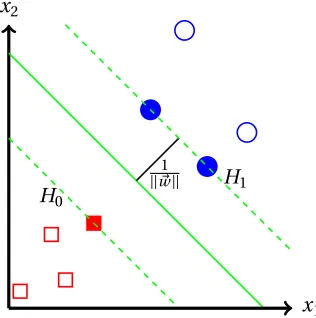
3.2.1 Linearly Separable Case

x2

1

||w~||

H0

H1

x1

Figure 3.2: An example of a linearly separable binary problem with SVM.

SVMs were originally designed, like LDA, for binary classification and prediction. Any unknown observationx~belongs to one of two classes,y0ory1, and so the SVM method finds a separation

hyperplane

g(x) =w~·x~+b

(28)

H =w~·x~+b, classification is determined by the decision hyperplane g(x) =







~

w·x~+b≥1 ifx~∈y1 ~

w·x~+b≤ −1 ifx~∈y₀

(3.18)

which, using the class indicator valuesy₁=1 andy₀=−1, can also be written in combination as yi(w~·x~+b)≥1 fori=0, 1. (3.19)

We define the hyperplanesH0andH1

H0: x~·w~+b=−1, (3.20)

H₁: x~·w~+b= +1 (3.21)

such that any points that lie alongH0orH1are the defined support vectors. Since the distance

from origin toH0is |−_||1w−_~||b| and from the origin toH1is|1_||−w_~b|||, the distance between the two that we

are trying to maximize is _||_w2_~_||. Thus, in order to maximize the distance, we have to minimize||w~||. Combining that with (3.18), the optimization problem is

min1 2||w~||

2_, _(3.22)

subject to yi(w~·x~+b)≥1, fori=1, . . . ,N. (3.23)

Because||w~||has a square root, it is much simpler to optimize 1₂||w~||2_{, which becomes a quadratic}

problem that can be solved using Lagrange multipliers[24]. The form of the Lagrangian is

L=1 2||w~||

2

−

N

X

i=0

αi[yi(w~·x~i+b)−1], (3.24)

whereαidenotes the Langrange multipliers. MinimizingLrequires four Karush-Kuhn-Tucker (KKT)

conditions[47]to be satisfied

Lw_~=0, (3.25)

Lb =0, (3.26)

αi≥0, i=1, . . . ,N, (3.27)

(29)

In combination with (3.24), we find

~

w=

N

X

i=1

αiyixi, (3.29)

N

X

i=1

αiyi=0. (3.30)

The Langrangian duality can be written in the Wolfe dual representation form, that is

max 1 2||w~||

2

−

N

X

i=0

αi[yi(w~·x~i+b)−1], (3.31)

subject to w~=

N

X

i=1

αiyixi, (3.32)

N

X

i=1

αiyi=0, (3.33)

αi≥0, (3.34)

which is equivalent to

max

N

X

i=1

αi−

1 2

N

X

i,j=1

αiαjyiyjx~i·x~j, (3.35)

subject to

N

X

i=1

αiyi=0, (3.36)

αi≥0. (3.37)

Whenαi>0, thenx~iis a support vector and the optimal separation hyperplane is

~

w=

n

X

i=1

αiyix~i, (3.38)

(30)

multiplierαi with corresponding support vectorx~iand labelyi, we find

αi[yi(w~·x~i+b)−1] =0 (3.39)

yi(w~·x~i+b)−1=0 (3.40)

y_ix~_i·w~+y_ib=1 (3.41)

b= 1

yi(

1−yix~i·w~) (3.42)

b=yi−x~iw~ (3.43)

b=yi− N

X

j=1

αjyjx~j ·x~i. (3.44)

Having foundw~andb, the classification function is

g(w) =sign(w~·x~+b) (3.45)

=sign

_n X

i=1

αiyix~i·x~+b

. (3.46)

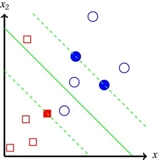
3.2.2 Nonseparable Case

While SVMs work very well for data that is linearly separable, the reality is that most data is not so easily separated. When a linear hyperplane cannot be drawn between the two classes, it is the nonseparable case, and requires a reformulation of the problem. In this instance, we can still use SVMs to classify unknown points, but need to account for any error. To do so, we know thatH₀and H1have the forms

~

w·x~i+b=±1, (3.47)

and the distance between them is the margin of size_||_w2_~_||. As shown in Figure 3.3, any training data ~

xiwith associated class labelyi belongs to one of three cases:

• x~_iis outside the margin, correctly classified, and therefore satisfies the inequality yi(w~·x~i+b)≥1.

• x~iis correctly classified but within the margin, satisfying the compound inequality

0≤yi(w~·x~i+b)<1.

• x~_iis incorrectly classified, satisfying the inequalityy_i(w~·x~_i+b)<0.

(31)

x2

x₁

Figure 3.3: An example of a nonseparable binary problem with SVM.

yi(w~·x~i+b)≥1−ξi, (3.48)

where the first case hasξi=0, the second case has 0< ξi≤1, and the third case hasξi>1. The

optimization problem now becomes

min1 2||w~||

2₊_C

N

X

i=1

ξi, (3.49)

subject to yi(w~·x~+b)≥1−ξifori=1, . . . ,N, (3.50)

ξi≥0 fori=1, . . . ,N, (3.51)

where C is an error parameter that determines how much emphasis is placed on maximizing the margin of the hyperplane versus reducing the number of misclassified data points. The Langrangian method still works for this optimization. The new form is

L=1 2||w~||

2₊_C

N

X

i=1

ξi− N

X

i=1

µiξi− N

X

i=0

(32)

with the respective KKT conditions

Lw_~=0 orw~= N

X

i=1

αiyix~i, (3.53)

Lb=0 or N

X

i=1

αiyi=0, (3.54)

L_ξ_i =0 orC−µi−αi=0, i=1, . . . ,N, (3.55)

αi[yi(w~·x~i+b)−1+ξi] =0, i=1, . . . ,N, (3.56)

αi≥0, i=1, . . . ,N, (3.57)

µi≥0, i=1, . . . ,N, (3.58)

as well as the corresponding Wolfe dual representation

max 1 2||w~||

2₊_C

N

X

i=1

ξi− N

X

i=1

µiξi− N

X

i=0

αi[yi(w~·x~i+b)−1], (3.59)

subject to w~=

N

X

i=1

αiyixi, (3.60)

N

X

i=1

αiyi=0, (3.61)

C−µi−αi=0, i=1, . . . ,N, (3.62)

αi≥0,µi≥0, i=1, . . . ,N. (3.63)

Using the equality constraints substituted into the Lagrangian (3.52), we find the maximization with new conditions

max

N

X

i=1

αi−

1 2

N

X

i,j=1

αiαjyiyjx~i·x~j, (3.64)

subject to

N

X

i=1

αiyi=0, (3.65)

0≤αi≤C. (3.66)

As in the separable case, we use the KKT conditions to solve forb. Combining the two equality statementsC−µi−αi=0 andµiξi=0, we findξi=0 ifαi=C. Thus, using any value satisfying

(33)

solution forb is the same as the separable case, and the decision function

g(w) =sign(w~·x~+b), (3.67)

where b=yi− N

X

j=1

αjyj(x~j ·x~i), (3.68)

is also the same as in the separable case, with the only additional constraint being that the Langrange multipliersαiare bounded above byC [47].

3.2.3 Kernel Function

In an effort to prevent the need for any error in the classification, we can try to make the data linearly separable to use with SVM. This technique depends on using the kernel "trick," a method using a function, denotedK(xi,xj), to map the original input data into a higher dimensional space,

ideally taking it from the nonseparable case (and thus requiring the slack error variable discussed previously) to a linearly separable case[11, 27]. There are a variety of functions that can be used in this mapping, an example of which is shown in Figure 3.4, but a few are the most commonly used:

Linear: K(x~i,x~j) =x~i·x~j, (3.69)

Polynomial: K(x~i,x~j) = (γ ~xi·x~j+b)p, (3.70)

Sigmoid: K(x~i,x~j) =tanh(γ ~xi·x~j+b), (3.71)

Gaussian: K(x~i,x~j) =exp(−γ||x~i−x~j||2). (3.72)

Because all of the training data is used in the optimization functions as inner productsx~_i·x~_j, then these functionsK(x~i,x~j)can be written as the dot product of the functionsΦ(xi)·Φ(xj)that

maps data from the original input dimension to some higher dimensional space, i.e.,

Φ:Rm→Rn, (3.73)

wheren>m. Replacing every inner product in the optimization withK(x~i,x~j), then the

(34)

Figure 3.4: Example of a kernel function mapping.

dimensional[27]. Without loss of generality, we assumeγ >0 andx~∈Rm, then

K(x~i,x~j) =exp(−γ||x~i−x~j||2) (3.74)

=exp(−γ(x~i−x~j)2) (3.75)

=exp(−γ ~x_i2+2γ ~x_i·x~_j−γ ~x2_j) (3.76)

=exp(−γ ~x_i2)exp(γ ~x_j2)exp(2γ ~xix~j) (3.77)

=exp(−γ ~x_i2)exp(γ ~x_j2)

1+

v t2γ

1!x~i

v t2γ

1!x~j+

v t4γ2

2! x~i

v t4γ2

2! x~j+· · ·

(3.78)

=Φ(x~i)·Φ(x~j), (3.79)

where

Φ(x) =exp

1,

v t2γ

1!x,

v t4γ2

2! x

2_{, . . .}

. (3.80)

(35)

training algorithm withK(x~i,x~j), so the maximization becomes

max

N

X

i=1

αi−

1 2

N

X

i,j=1

αiαjyiyjK(x~i,x~j), (3.81)

subject to

N

X

i=1

αiyi=0, (3.82)

0≤αi≤C, (3.83)

and the final decision solution is

g(w) =sign

_N X

i=1

αiyiK(x~i,x~j) +b

, (3.84)

where b=y_i−

N

X

j=1

αjyjK(x~i,x~j). (3.85)

3.2.4 Multi-Class SVM

The extension of binary SVMs to a class method has led to two common approaches to multi-class multi-classification. For a problem withN distinct classes, the one-vs-all (OVA) method createsN SVMs, and places the unknown value in whatever class has the largest decision function value.

For our model, we used the one-vs-one (OVO) method, which createsN(N −1)/2 SVMs for classification. For a set ofp training data,(x1,y1), . . . ,(xp,yp)where xl ∈Rn,l =1, . . . ,p andyl ∈

{1, . . . ,N}is the class label forx_l, then the SVM trained on theith_and_jth_{classes solves}

min

wi j_,_bi j_,_ξi j 1 2(w

i j₎T_wi j₊_CX

`

ξi j_` , (3.86)

where(wi j)Tφ(x_`) +bi j≥1−ξi j_` ify_`=i, (3.87) or(wi j)Tφ(x_`) +bi j≤ −1+ξi j_` ify_`=j, (3.88)

ξi j

` ≥0, (3.89)

whereΦ(x)is the radial basis function used to map the training dataxi,j to a higher dimensional

space andC is the penalty parameter[29]. After all comparisons have been done, the unknown value is classified according to whichever class has the most votes from the assembled SVMs.

(36)

Figure 3.5: A visual representation of the one-vs-all method (thin lines) compared to the one-vs-one method (thick line) from[2].

the OVA method leaves a gap where the classification algorithm can fail to place an unknown value, but since the OVO method does not have any blind spots, we used it for our classification.

3.3 Classification Trees

While linear discriminant analysis and support vector machines are geometrically-based methods, decision trees do not rely on optimizing the distance between classes or the projections of classes. Introduced by Breiman et al., classification and regression trees (CART) are binary decision trees built using both continuous and categorical data[9]. Both classification and regression trees are constructed (or grown) the same way, examining all possible splits of all possible features, and then making a binary decision, yes or no, if the condition is satisfied or not. Figure 3.6 shows a basic example of what a single decision tree may look like for pitch prediction.

(37)

Balls

FB

≥2

Inning

Pitch Count

FB

≤₄₀

CH

>40 and<80

CU

≥80

>4

SI

≤4

<2

Figure 3.6: Basic Classification Tree for Pitch Selection.

is known as total impurity.

To build a classification tree, all features are considered at first. The algorithm examines each feature and finds which one, when split, will reduce the impurity of the tree nodes the most. Once the feature is selected, then the threshold that reduces impurity the most is found, and the process is repeated until either some impurity threshold is determined or all the end nodes (leaves) are pure, i.e., they only contain one class of data. Impurity can be found by different measures, but the one we employ is the measurement used in the MATLAB implementation of classification trees, the Gini diversity index (gdi), which can be represented as

I =1−

N

X

i=1

p2(i), (3.90)

wherep(i)is the fraction of each classi=1, . . . ,N as a total part of the number of observations at that node. Using the gdi to determine the impurity is the same idea as judging the total accuracy of the tree by randomly selecting an answer from the distribution of each class at the end leaf node[36]. During the training process, the impurity threshold is generally set to be small enough so that all leaf nodes are pure. An example of two different splits with two different levels of impurity are shown in Figure 3.7.

(38)

Figure 3.7: Two sample splits for a decision tree with four unique classes. The split on the left is better, as total impurity is lower due to having higher proportions of fewer classes present in each leaf, minimizing the gdi. Taken from[30].

3.3.1 Random Forests

Introduced by Brieman in 2001, random forests are used to reduce error by grouping together large numbers of classification trees. Random forests are an extension of the ensemble approach for decision making, which involves growing multiple trees on the full data set and letting a majority vote determine the class (we will discuss this in more depth later in the chapter). Random forests differ in that each tree is grown on a random subset of the training data without replacement. The use of these random subsets is known as bootstrap aggregation (or bagging). Parameter selection may be done randomly as well, selecting from some numberK of the best features and the best splits to grow the tree[8].

For some testing set dataXwith corresponding labelsY, we denote the ensemble set of random forest classifiersh1(x),h2(x), . . . ,hK(x), each trained with random selections fromX. Breiman defines

the margin function

mg(X,Y) =avkI(hk(X) =Y)−max

j6=Y avkI(hk(X) =j), (3.91)

whereI(·)is the indicator function. This margin function is a measure of how much the number of average votes for the correct classY is greater than the number of average votes for any other (incorrect) class. The greater the margin function, the greater the confidence in classification there is. Breiman defines the generalization error as

PE∗=PX,Y(mg(X,Y)<0), (3.92)

(39)

Given a large amount of trees, then from the Strong Law of Large Numbers and the structure of the trees themselves, we find:

Theorem 3.3.1. As the number of trees N increases, for almost surely all sequencesΘ₁, . . . ,Θ_N, then

PE∗converges to

PX,Y(PΘ(h(X,Θ) =Y)−max_j

6

=Y PΘ(h(X,Θ) = j)<0). (3.93)

The proof is shown in[8]. This theorem shows why the random forest approach does not overfit as more and more trees are added, but instead limit the generalization error. The resistance to overfitting is a large strength of the random forest formulation, as opposed to a single decision tree, which can be overfit as more and more training data is added and the tree grows larger and larger.

3.4 DIRECT Algorithm

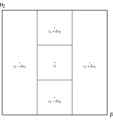
To save time and skip performing a brute force grid search to determine optimal parameters for the SVM and LDA methods, we used DIRECT. The DIRECT algorithm was developed in an effort to combat issues faced by Lipschitzian optimization: a nontrivial generalization to dimensions ofN >1 and the need for an estimate of the Lipschitz constant. DIRECT is easily extended into multiple dimensions, and requires no initial parameter estimate, just an error measurement functionf.

The algorithm begins by transforming the domain of the optimization problem to the unit hypercube

Ω={x∈RN : 0≤x≤1},

whereN is the number of parameters being estimated. DIRECT marks the center of this spacec₁ and findf(c1), the error function value at the center. Next, it divides the hypercube into potentially

optimal hyper-rectangles (leading to the name, DIviding RECTangles) by evaluating the error func-tion at the pointsc₁±δeifori=1, . . . ,N, whereδis one-third the length of the side of the hypercube

andeiis theith unit vector. The algorithm initializes by choosing to leave the best function values

in the largest space, defining

wi=min f(c1+δei),f(c1−δei)

, (3.94)

for 1≤i≤N. DIRECT then divides the dimension wherewiis smallest into thirds, leading toc1±δei

as the new centers of the new hyper-rectangles, repeating the split for each subsequently largerwi

to find an initialization, an example which is shown in Figure 3.8.

(40)

p1 p2

. c1

. c1−δe2

. c1+δe2

. c1−δe1

. c1+δe1

Figure 3.8: An example initialization of the DIRECT method for two parameter optimization.

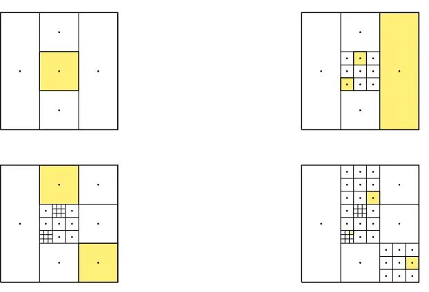
minimize the function are identified as potentially optimal, which are then split and tested them-selves. These potentially optimal rectangles may be found using a few observations defined in[20]:

• If hyper-rectanglei is potentially optimal, thenf(ci)≤f(cj)for all hyper-rectangles that are

of the same size asi, i.e.,d_i=d_j.

• Ifdi≥dkfor allkhyper-rectangles, andf(ci)≤f(cj)for all hyper-rectangles such thatdi=dj,

then hyper-rectanglei is potentially optimal.

• Ifdi≤dkfor allkhyper-rectangles, andi is potentially optimal, thenf(ci) =fmin.

Once a potentially optimal hyper-rectangle is identified with centerc_i, DIRECT continues to divide it into small hyper-rectangles along the jth_{dimension, evaluating at the points}_c

i±δiej,

using a determination similar to the initialization, i.e.,

wj =min f(ci+δiej),f(ci−δiej)

, (3.95)

(41)

. . . . . . . . . . . . . . . . . . . . . . .. . . . . . . . . . . . .. . . . . . . . . . . . . . . . . . . . . . . .

Figure 3.9: An example of four iterations of the DIRECT algorithm. Possible optimal rectangles are high-lighted in yellow for each iteration.

Cross validation error is a method of model validation that uses a majority portion of the data to fit the model and the remaining fraction to test it. Cross validation is repeated at least twice on different splits of the data (called n-fold cross validation for n different splits) to determine a theoretical level of accuracy for the model. For DIRECT, we use the error of the five-fold cross-validation estimate as the value we are trying to minimize over a two dimensional rectangle of parametersC andγfor the SVM and the regularization parametersγandδfor LDA. Some experiments were attempted using different class weights as parameters, but the computation time was prohibitively increased for little to no improvement in results.

3.5 Committee Approach

(42)

same subset. This can be accomplished by varying the hyper parameters for the individual models, or changing the error threshold for the committee members, among other ways[1]. The committee approach is recognized to work better than individual models for three reasons[15]: statistically, computationally, and representationally:

1. Statistical reason: Any machine learning method is searching a possible hypothesis space H in an attempt to find the best hypothesis. If, however, the amount of training data is too small compared to the size ofH, then the method could find multiple hypotheses inH that have the same accuracy on the training data. By constructing multiple different classifiers and using them in an ensemble, this approach "averages" out the votes and therefore reduces the risk of finding the wrong class.

2. Computational reason: In order to find the best way to classify, many methods perform a local search that can possibly get stuck in a local optima (the best example being neural networks using gradient descent training). Even when there is enough training data to avoid the statistical pitfall, by combining multiple different classifiers, the various local minima each gets stuck in can be "averaged" to minimize error.

3. Representational reason: When the actual classification function cannot by represented by any hypothesis inH, then the weighted sums of the hypotheses found by the individual members of the committee can expand the search space.

A visual representation of the three reasons for the success of the ensemble method is shown in Figure 3.10. Just as there are a wide variety of machine learning classifiers, there are a variety of ways methods can be combined in an ensemble committee, as detailed in[15]:

1. The Bayesian Voting ensemble method uses the sum over all hypotheses functionh(x)∈H, each weighted by its posterior probabilityP(h|S), whereSis the training sample.

2. The Training Set Manipulation method of ensemble construction is a relatively straightforward approach, simply giving each member of the committee a different random subset of the training data.

• The most common way of doing this is taking a set fraction of the original dataset drawn randomly with replacement, called bootstrap aggregation, or bagging, giving each member of the committee an equal vote.

(43)

Figure 3.10: A visual representation of the three reasons why an ensemble method works better than a single one, taken from[15]. Each committee member is represented in blue, with the true classifier labeled in red.

• A third way of manipulating the training data is the ADABOOST algorithm, which oper-ates similarly to bagging but associoper-ates a weight with each committee member’s hypoth-esis.

(44)

4. The Output Target Manipulation method uses derived labels with error-correcting output to determine different committee members that have been trained on different output subsets.

5. The Randomness method uses random initializations to create different members of the ensemble, usually applied to neural network algorithms that, because of the backpropagation training method, end up with different weights given different initializations.

The use of a committee approach for Classification Trees and SVMs is not novel, having been used for binary SVM classification in[3, 4], but to our knowledge it has not been extended to multi-class prediction outside of a survey paper[22], and certainly not in the realm of pitch prediction.

We decided to apply bagging to our methods, allowing each classifier an equal vote in the end decision, so our committee of ten models decides according to the pitch type that has the most votes. For our committee approach, we run DIRECT ten times on random permutations of the training set, getting ten differentC andγvalues for SVM and ten different regularization values (γ andδ) for LDA. We use 100 trees in each iteration of TreeBagger, as trying to optimize the number of trees in each random forest was computationally inefficient and resulted in no accuracy increase. In the case of a tie, five extra models are trained, using a random value between the minimum and maximum values of the ten original parameters.

3.6 Contributions

(45)

CHAPTER

4 PREDICTION RESULTS

We implemented all of our experiments in MATLAB, using the statistics and machine learning toolbox for random forests and linear discriminant analysis and the libsvm software[11]for support vector machines. Due to the committee method, we used the parallel computing toolbox on a remote server to train each of the ten committee members at the same time to reduce computation time.

To establish a value for comparison, we found the best "naive" guess accuracy, similar to that used in[23]. We define this naive best guess to be the percent of time each pitcher throws his preferred pitch from the training set in the testing set. Consider some pitcher who throws pitch types 1, 2, 4, and 5 with distributionP ={p1,p2,p4,p5}where

P

pi=1, and his preferred training

(46)

4.1 Comparison of Methods

Because of the way the committees were built for each pitcher, the LDA parametersγandδand the SVM parametersC andγvaried across each member of the ensemble. Table 4.1 shows the average values for each parameter across all of the pitchers tested.

Table 4.1: Average parameters values for all committee members for all pitchers.

LDA Parameters SVM Parameters

γ δ C γ

0.0882 0.0932 43.1814 0.0688

Table 4.2 shows the prediction results from each individual method (the random forest method is labeled 100 CT). Results for every individual pitcher tested are given in Appendix A. The number of pitchers we predicted better than naive is given, as well as the percentage of the 287 total pitchers that number represents. The average prediction accuracy is shown, given along with the overall average improvement over the naive guess, denoted ¯PI, the average improvement for those pitchers

who did beat the naive guess, denoted as ¯P_B, and the average amount the pitchers who did not beat the naive guess failed by, denoted by ¯PW. Given the number of pitchersN with respective prediction

valuePi and naive guessGi, the number who did better than the naive guess,NB, the number who

did worse than the naive guessN_W, we find

¯ PI =

N

P

i

Pi−Gi

N ,

¯ PB=

NB

P

i

Pi−Gi

NB

,

¯ PW =

NW

P

i

Pi−Gi

NW

.

We also give the average range of accuracy between the most and least accurate members of each committee as well as the average time for each pitcher’s model to be trained and tested.

(47)

Table 4.2: Comparison of prediction results for each method.

Value LDA SVM 100 CT

# of Predictions>Naive 263 251 282 % of Predictions>Naive 91.64 87.46 98.26

Prediction Accuracy (%) 65.08 64.49 66.62 ¯

PI (%) 10.70 10.11 12.24

¯

PB (%) 13.26 12.38 12.52

¯

P_W (%) -9.08 -5.40 -1.15

Range of Committee (%) 1.52 3.02 2.22

Time (s) 22.75 2,383.8 72.05

SVM by a wide margin. Basing the judgement solely on how many pitchers were predicted better, the random forests were near-perfect, leading the average prediction accuracy and improvement to also be higher. LDA outperforms the random forests only when we examine the average improvement for those pitchers who we are able to beat the naive guess for, but conversely also has much worse performance for the pitchers we do not beat the naive guess for. At this stage, we undertook further comparative analysis to determine if the random forests were the best method overall.

4.2 Results Analysis

4.2.1 Results by Type of Pitcher

Because our data set featured both starters and relievers, we wanted to examine if there was any difference between the prediction accuracy for starters against relievers. Due to the fact that starters will play many more innings (and therefore throw more pitches), the average starter had 6,390 pitches over the three seasons, and the average reliever threw 2,812 pitches over all three seasons. The average naive guess for starters was 51.73%, while for relievers it was 57.28%, indicating that relievers relied on a preferred pitch more than starters did, which makes sense given the nature of a reliever’s job: pitch for a short amount of innings, get a lot of strikes and outs, and do so using a pitch they have the most control over. Table 4.3 shows the difference in the random forests prediction accuracy for starters versus relievers for all three methods considered.