THE LOCATION OF VIABILITY GENES WITHIN A TESTCROSS FRAMEWORK

THE

LOCATION OF VIABILITY GENES WITHIN A TESTCROSS FRAMEWORK

WILLIAM CHAPCO

Department of Biology, University of Saskatchewan, Regina, Canada

Manuscript received January 4, 1971 Revised copy received August 23, 1971 Second revision received October 12, 1971

ABSTRACT

The maximum likelihood method is applied to the problem of estimating the positions and effects of viability genes. Whenever testcross linkage data in- dicate the presence of differential viability, it is hypothesized that there exists one viability gene between each marker. Estimation is possible only for two- p i n t data since the number of independent expectation expressions is less than the number of parameters for three or more markers. I t is pointed out that within the two-point testcross system, it is impossible to distinguish between pleiotropic effects of the marker genes and the effect of a middle viability gene, if existent. The methods outlined will he useful in their application to experiments specifically designed to locate induced viability genes.

seems reasonable to believe that most visible mutant genes are pleiotropic

‘Tor reduced viability since they do represent a deviation from the develop- mental norm for an organism (SCHMALHAUSEN 1949, MUNTZING 1967). Naturally, the extent of the disruption of the genetic balance depends upon the role of the normal alleles in development. FORD (1934) points out that linkage of a mutant gene to viability genes may be another explanation for the marker’s apparent loss of viability. However, he states further: “That such an assumption is not generally tenable can be proved in those instances where the same mutation has occurred more than once. Not only the primary but also the secondary effects have then appeared again.” Yet, there are instances in which certain mutants are not always associated with differential viability. For example, the crossvein- less gene cu in Drosophila exhibits normal viability in data reported by SINNOT, DUNN and DOBZHANSKY ( 1950) whereas the experiments of

PARSONS

(1 95 7) and CHAPCO (1967) indicate that the gene lowers viability. Also higher viabilities for some mutants have been achieved by placing them on different genetic back- grounds ( CARVER 193 7).

The usual procedure of dealing with differential viability when estimating map distances from intercross or testcross data is to assume that the markers under consideration are pleiotropic f o r reduced survival (BAILEY 1961). The original purpose of this paper was to present a n alternative view based on linkage (Model 1) rather than on pleiotropy (Model 2) and at the same time provide a means by which viability genes could be located within a testcross framework.

However, it will be demonstrated that the two views cannot be resolved. Also, it will be shown that for testcrosses involving thrce or more markers, it is im- possible to estimate viability gene positions.

MODEL 1

Assume that two homozygous strains, A1A2.

...

A, (wild strain) and ala2

....

a, (mutant strain carrying s linked visible markers none of which affect viability) are crossed followed by testcrossing the

F,.

Between each pair (ai,ai+,) let there be a viability gene, Vi1

( i

= 1,2,

...

s-1). Corresponding to each Vi1 there is a homologous Vi2 gene on the wild chromosome. Thus the

F,

genotype is:

A,V12A2V,2A3

. . .

A,-,V2,-,A, alV11a2V21a3

. . .

as-lV1s-las

Let pi and qi be the recombination fractions between ai and Vi1, Vi1 and ai+,, respectively

( i

= 1,2,

. . .

s-1). It will be assumed that crossovers in different segments occur independently. Let the relative viabilities of Vi2Vi1 and VilVi’

(1961) in which the viability of a genotype is expressed as a ratio relative to a standard genotype.

The expected proportions and the observed number of testcross progeny in each of the 2, phenotypic classes are denoted as follows:

be

xi

and yi = 1

-

xi

(i

= 1,2,

...

s-1). This definition differs from BAILEY’S

Phenotypic class

Expected Observed

proportion number

A,A2..

. .

A,-,A, mll

. . . .

11 n11

. . . .

11

A , A 2 . .

. .

A,-l a, mll

. . . .

12 n,,

. . .

.,3

A,A, as-lAs mll

. . . .

2 1 n11.

. .

. 2 1 A,A2.

. . .

as-l a, mll

. . . .

2 2 1211.

. .

. 2 2

. . . .

a, a2

. . . .

as-l a, m Z 2 .

. . .

2 2 n22 *

-

.

. z z

where the sum of the m’s equals one. Each m and n has s subscripts such that the i’th subscript is a 1 if the i’th symbol in the corresponding phenotypic class is a n A; it is a 2 if the i’th symbol is a n a. The general phenotypic class can be repre- sented by:

S

II Gi = GIG2

. . . .

G, i=1

and its expected frequency by mg . , ,

.

where Gi={

12 $

LOCATING VIABILITY GENES

t i j k = xi [2--j

+

( - 1 ) j pi]

[2-k

+

4iI

Wijk = y i ri-1

+

pi] [k-l

+

(-1) k + l

4,]

.

.

and

It is claimed that for s

>

2 that

321

where

For example, when s = 2

Phenotype Expected proportion

- -

-A1A2 Ala2 alA2 ala2

mll = ulll = xl( l-pl) (l-ql) - ylplql

m12 = ul12 = x1 ( 1 -pl) q 1

+

ylpl ( 1 -ql) mzl = ulZl = x2pl ( 1-9.1)

+

yl( 1 --PI) 41

mZ2 = ulZ2 = x l p l q l

+

yl(l--pl) (l--ql)

In this case D2 = 1.

The proof of (1) follows. Individuals possessing the pair G,G,+l are either

G,V,'G,+, or G,VilG++l and these 'segments' are produced in frequencies pro- portional to teg and w , ~ , ~ , + ~

,

respectively. More generally (for i=1,2,.

.

.

,

s - l ) , G,V,"G, +l types are proportional to:

% I f 1

+

( k b - 1 )wzPp,+l

- (2-k

1

tzg*g, + 1 -

hzgzBz

(k,

= 1,2; i=1,2,.

.

.

. ,

s-1).

Therefore, the genotype G1VlklG2V2kzG3

. . . .

G,-1V8-1k~-G8

is proportional to

8-1

2 1 h * g z g z

+

lk%

Hence the phenotype,

,fi

Gi is proportional to the multiple sum

%=l

8-1 8-1

8

Therefore, the frequency of the phenotype,

,n

Gi is

a = 1

8-1

-

mg1g2. . . . B8

-

igl

U i g i g i f l / D 8

MODEL 2

The pleiotropic model will be described so that it can be compared with Model 1. Let each ai gene be pleiotropic for reduced viability such that the relative viabilities of Azaz and arai are z , and 1-2, (i=1,2,

. . . .

,

s), respectively. Set the distance between ai and ai+l equal to c, (i=1,2,.

.

. .

s-1). Therefore, the ex-

pected frequency of the general genotype,

(

,il

G,

)

is

where

z L if G, = A,

1-2, if G, = a,

c, if G,G,+l = or f . l =

{

and

1

I-c, if G,G,+l = A,A,+l or a L a z f l

i-i =

L,

is the normalizing factor. The proof of (2) will not be given here since Model

2 is a n obvious extension and modification of the two-point differential viability modelinBAILEY (1961, p. 51).

ESTIMATION

There are 3(s-l) parameters (xi, p i and qi; i=l,2,

.

.

. . ,

s-1) to be estimated in Model 1. Estimation is possible if at least 3(s-l) of the 2s expectations are independent. It is shown in Appendix 1 that there are at most 2s-1 functionally independent m’s. Since 2s-1

<

3(s-l), estimation of the parameters is possible only for s=2 or two-point testcrosses.

When s=2, there are 3 degrees of freedom available to estimate xl, pl and

41;

none are left for making a test of goodness-of-fit. Maximum likelihood estimators can be obtained by equating the expected numbers to the observed numbers. When this is done, the following estimators are obtained:

(n11Sn21) - 21n

n ( 1-255) and

G1=

(n11fn12) - 21n n (1 -2&)

$1 = (3)

Instead of carrying out algebraic differentiation in order to obtain the elements the information matrix and hence the elements of the covariance matrix, partial derivatives can be obtained numerically (REED 1969).

LOCATING VIABILITY GENES 323

Z m = 1, mlll/mllz = m d m z l z and mlzl/mlzz = m2z1/mzzz. (4) The experimenter could test these last two relationships by performing x 2 tests on the contingency tables:

respectively.

If one is willing to utilize tabulated map distances, estimation for s=3,4 or S(or more, but one should check as in (4) to see if the number of independent

m’s is exactly 29-1) is possible. The number of parameters would be reduced from 3(s-l) to 2(s-l). There would be one degree of freedom left for making a test of goodness-of-fit. Thus if there is no interference and if c, is the recombi- nation fraction (transformed from the tabulated map distance by HALDANE’S

(1919) mapping function) between a, and a,+, (i=1,2,.

. . .,

s-1), then p, and qi are related by c, = p z

+

qi - 2p,qi (BAILEY 1961). Although this procedure could be carried out for Drosophila and other organisms for which there exist tabulated map distances there are dangers in its application. It is well known that map distances are influenced by such factors as temperature (PLOUGH 1921)’ age of female (BRIDGES 1927), genetic background (LAWRENCE 1958), and cyto- plasm (THODAY and BOAM 1956). Therefore, it is unlikely that the tabulated distances would be exactly the same as those in the experimental material at hand. However, if one is willing to risk this possibility, for s=3, initial estimators of xl, pl, xz and

qz

can be obtained by solving:

C1

= 0.5 - 0.5 v‘1-4C

21 =

,

Gi(k(1

-61)

-61)

(l-fi1-ij1) -k,(fi1-41) 7

4,

= 0.5 - 0.5 d 1 - 4 F

_,

where

These initial estimators were obtained by equating the observed frequencies to

the expected frequencies after letting pl -t q1 - 2plql = c1, and p 2

+

q2 -

2p2qz = cz. Estimation can then proceed iteratively using efficient scores (RAO 1952). A numerical procedure (REED 1969) can be used to obtain scores and the elements of the information matrix.

APPLICATION O F MODEL 1 A N D COMPARISON WITH MODEL 2

Two-point data: Models 1 and 2 were applied to some of the early Drosophila

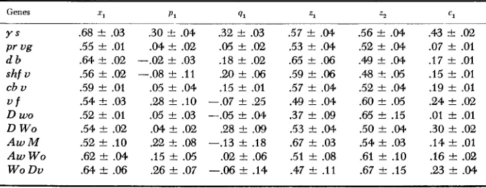
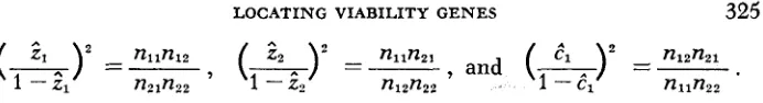
linkage experiments of MORGAN and BRIDGES (1916) and BRIDGES and MORGAN (1919) and some tomato data of BUTLER (1960) in which differential viability was present. The experimental data are presented in Table 1 and the maximum likelihood estimators of zl, pl, ql, zl, zz and c1 and their standard errors in Table 2.

(The

M.L.E.

of zl, z2 and c1 were obtained by solving TABLE 1

Two-point linkage data

Genes

Drosophila

Y S

Pr vi?

d b

shf U

cb U

u f

Tomato D W O

D W O A w M

A w WO

W O Du

-41-42 373 1539 495 365 697 273 1367 318 1568 148 66

225 21 9

119 116

108 55

72 46

151 125

72 91

6 19

132 115

221 270

19 28

9 21

226 1238 275 282 490 229 1250 270 1440 92 36

TABLE 2

Estimates of parameters in models I and 2

Genes 2;

Y S Pr ug d b

shf U

cb U u f

D W O

D W O

A w M

A w WO

WO Dv

.68 f .03 .55 f .01

.64 t .02

.56 f .02

.59 t .01 .54 t .03 .52 f .01 .54 f .02 .52 t .10 .62 t .04

.64 -+ .06

p1

.30 F .04 .04 f .02

~~~

-.02 f .03 -.08 t .ll .05 f .04 .28 f .IO .05 f .03 .04 t .02 .22 f .08 .I5 f .05

.26 f .07

91

.32 f .03

.05 f .02 .I8 f .02 .U) f .06 .I5 f .Ol -.07 f .25

-.05 t .04

.28

*

.09

-.I3 f .I8 .02 f .06

-.06 f .I4

7-1

.57 t .04 .53 t .04

.65 f .06 .59 t .06

.57 f .04 .49 f .04 .37

*

.09 .53 f .04 .67 f .03 .51 F .08 .47 f .I1

22

.56 t

.52 t

.49 f .48 S .52 f .60 t

.65 t

.50 f

.54 t

.61 t

.67 f ~ .04 .04 .04 .a5 .04 .a5 .I5 .04 .03

. I O

.I5

c1

.43 t .02

.07 f .01 .I7 f .01 .15 t .01 .I9 f .01 .24 t .02

.01 f .01 .30 f .02 .I4 F .01 .16 f .02

.w

t .04

LOCATING VIABILITY GENES 325

(i")*

=- nllnzl

,

and

(A)*

=-.

nlznzl

1 -z1 n21n22 1 - 2 2 n12n22 1 --Cl n11n2?

("-)*=-,

nllnlz

A one-to-one relationship between 2,,

el,

Q1,

and

&,

2,, t1,

does exist, as suggested by a reviewer. A rather complex set of associations can be obtained by replacing the n's in (3) by their expected values in terms of

&, &,

and 2,).

Models 1 and 2 cannot be resolved if both markers are pleiotropic. Conversely,

i f in fact a viability gene does exist between two markers, it will appear as if the two markers are affecting viability. This point is illustrated in Table 2 by gene sets 1 and 2 f o r each of which it would appear that both markers are pleiotropic or there exists a viability gene between the markers (Table 3).

If only one of the two marker genes is pleiotropic for viability, Models I and 2

coincide. For example if A, affects viability then p , = 0 (Model 1) and z2 =

%

(Model 2) give the same class expectations ( q l = 0 and z1 =

'/2

will also give the same expectations if A, is pleiotropic). The former situation implies that

m,,/m12 = m,?/m,, while the latter, m,,/mZl = m 2 2 / m 1 2 . These relationships can

be tested by appropriate contingency x 2 tests (x12 and x J 2 , respectively) being applied to the corresponding 'n values'. I t would appear (Table 3) that genes

d, shf, cb, f ,

D,

M ,

W O ,

and

Dv

arc pleiotropic for viability. Nevertheless, the question of very tight linkage remains.

No restriction has been placed on the possible values the estimators may take. For gene sets 3,4,6,7,9. and 11, negative estimates of

6,

and

e,

are obtained. Numerically, they are not statistically different from zero. If Model 1 is correct, negative values can be obtained by sampling and should be taken as zero in much the same way negative variance components are treated. If this is done, Model 1 coincides with Model 2 with only one marker pleiotropic for viability. Exami- nation of equations ( 3 ) reveals that imaginary values of

f,,

6,

and

Q1

would be obtained if ( r ~ , ~ - n ? ~ )

<

-C ( r ~ , ~ - n ~ ~ ) . This could result simply by sampling in

TABLE 3

Tests of the hypotheses

p, = O or zp = x ( x l z ) and q 1 = 0 or z1 =

x(x2*)

Genes X , Z x,?

YS

Pr ug

d b shf v

cb U

u f

D W O

D WO

A w M A w W O

W O Dv

14.0* * 20.1 * * 0.2 0.9 1.5 5.1 7.9- 0.0 8.6** 7.3**

11.4*+

17.4' * 32.2* * 51.9** 12.2** 16.4'*

TABLE 4

Three-point linkage data and tests of hypotheses q1 = 0 and p, = 0

Genes

sc cu U b PT ug a1 d p b

933 274 6 1 03 140

6 206 736 26.3’ 16.3 *

355 32 1 8 8 1 38 268 0.1 0.2

1365 529 13 149 21 1 17 448 a75 4‘46.4*

45.0’

* P

<

.01

which case boundary conditions ( p l 2 0, p l

<

i/z,

q1 2 0 , q1

<

i/z,

x1

>

1/)

could be incorporated into the above mentioned numerical iterative procedure (REED

1969). Alternatively. Model 1 might be incorrect and a model involving gene- gene interaction could be looked into.

Three-point data: Three sets of Drosophila three-point linkage data (Table 4) (taken from PARSONS (1957)

,

BRIDGES and MORGAN (1919) and CHAPCO (1967)

,

respectively) were tested

(x3?

and x4*) to see if they conform with (2) (Table

4).

In cases 1 and 3, the x2’s were highly significant implying the existence of factors not considered such as marker-marker interactions. I n case 2, estimation of zl, z2, p l and q2 (utilizing tabulated c1 and c,) was attempted but yielded esti- mators and standard errors of atrocious magnitude. Further investigation re- vealed that the data supported the hypotheses: ql = 0 (or

zl

= 0.5) and p? = 0 (or z2 = 0.5). These were tested by performing contingency

xz

tests on n111/n211 = n212/nlZl and nlll/nl12 = n122/n121, respectively. The x2’s were 0.14 and 0.10. It would appear that the middle marker pr is pleiotropic for viability. I t is con- cluded that effectively, two additional degrees of freedom (coming from the two functional relationships) were lost leaving only 5 - 2 = 3 df to estimate the four parameters zl, p l , z2, and q, and hence resulted in the obtaining of the in- admissible estimators.

DISCUSSION A N D USES O F M O D E L 1

LOCATING VIABILITY GENES 327

might be answered. Presumably, if viability genes do exist, recombination occur- ring during the construction of the various heterozygotes would disrupt the original associations between markers and viability genes. This could explain why the viability of the C U + gene relative to that of cu in PARSONS (1957) varied from a ‘neutral value’ of almost 0.50 to a significant 0.58 depending on the ar- rangement of genes in the parental heterozygote.

The methods of Model 1 could be applied in the following experiment designed specifically to locate induced viability mutations. The viability mutations would

be induced chemically or by ionizing radiation in a n isogenic multiply marked strain for which preliminary analysis had indicated that differential viability was absent. These mutations would be detected by standard techniques such as the

‘Cy/Pn’ method of detecting lethal and viability mutations in the second chromo- some in Drosophila. The outcome would be the creation of the same multiple- marker strain but possessing one or more viability mutations. Both treated and untreated strains would then be involved in a testcross with some wild-type iso- genic strain and followed by application of the methods outlined in Model 1. The linkage data from the original marker strain would serve as a control and would provide the experimenter with adequate values for each of the

ti's.

All this as- sumes that only one mutation is induced within a segment delineated by two markers. This is not an unreasonable assumption since the probability that more than one mutation is icduced within the same segment is small.

LITERATURE CITED

BAILEY, N, T, J., 1961 BRIDGES, C. B., 1927

BRIDGES, C. B. and T. H. MORGAN, 1919

Introduction to the Mathematical Theory of Genetic Linkage. Oxford

University Press, Oxford.

The relation of the age of the female to crossing over in the third chromo- some of Drosophila melanogaster. J. Gen. Physiol. 8 : 698-700.

Contributions to the Genetics of Drosophila melano-

gaster. 11. The second group of mutant characters. Carnegie Institute of Washington Publi-

cations 278: 123-304. Washington.

BUTLER, L., 1960 The linkage map of chromosome 2 of the tomato. Can. J. Botany 38: 365-379. CARVER, G. L., 1937 Studies on productivity and fertility of Drosophila mutants. Biol. Bull.

CHAPCO, W., 1967 Inheritance of fertility in Drosophila melanogaster. Ph.D. Thesis, University FORD, E. B., 1934 Mendelism and Evolution. Methuen and Company, Ltd., London.

HALDANE, J. B. S., 1919 Woods Hole 73: 214-220. of Toronto, Toronto, Canada.

The combination of linkage values, and the calculation of distance be- Genotypic control of crossing over on the first chromosome of Drosophila

Sex-linked Inheritance in Drosophila. Carnegie Institute

tween the loci of linked factors. J. Genet. 8 : 299-309. LAWRENCE, M. J., 1958

melanogaster. Nature 182 : 889-890.

of Washington Publications 237: 1-88. Washington, MORGAN, T. H. and C. B. BRIDGES, 1916

MUNTZING, A., 1967 PARSONS, P. A., 1957

Genetics: Basic and Applied. LTs Forlag, Stockholm.

An effect of gene arrangement on the recombination fraction in Drosophila

PLOUGH, H. H., 1921 Further studies on the effect of temperature on crossing over. J. Exptl. Zool. 32: 187-202.

RAO, C. R., 1952 REED, T. E., 1969

579-582.

SCHMALHAUSEN, I. I., 1949

SINNOT, E. W., L. C. DUNN and TH. DOBZHANSKY, 1950 THODAY, J. M. and T. B. BOAM, 1956

Advanced Siaiisiical Meihods in Biometric Research. Wiley, New York.

A general maximum likelihood estimation program. Am. J. Hum. Genet. 2 0 :

Fnciors of Evolution. Blakiston Company, Philadelphia.

Principks of Geneiics. McGraw-Hill,

A possible effect of the cytoplasm on recombination in Toronto.

Drosophila melanogasier. J. Genet. M : 456-461.

A P P E N D I X I

Proof that the number of functionally independent equations is at most 2s-I

is presented. From (1), the 28 expected frequencies, the m’s, are proportional to

,n

u ~ , ~ , ~ + ~ . There are 4(s-l) U’S altogether. Taking logarithms,

where

and 8-1

a = 1

Rlgz

. . . .

is proportional to

I:

Si, .,,

( 5 )

8 z 1 + 1

&,Pz

. . .

. gs =

1%

%,gz

. .

. . g8 ‘c6.g. = log u i 6 . g . 2 k+1

z % + I

(gi ’= 1,2;

i

= 1,2,

.

.

.

.

,

s-1)

The system

(5)

can be represented in matrix form:

R P , ~

Mz*,+(s-1)Si(s-i),1

where

S

and R are column vectors of the S and R elements and for s

>

2 it can

Be shown that

M

is of the recursive form:

where 2 k = 2 3 ,

0 0

0 0

and

LOCATING VIABILITY GENES

0 1 0 0

Bk;,

-

=[

io

1

0 1 0 0

ck,

_-

4 = 2

-

0 0 1

0 0 1

-

0 0 1

-

0

0

0 0 0 1 -

D;4=[

- 0 0

.

0 1

0 0 0 1 -

329

For s,= 2,

M

is the 4 X 4 identity matrix.

Mk,

4(a-2) is a matrix of coefficients

that relates the R's and S's for s-I markers.

It is claimed that the rank of M2k,4(8-l) is 2s. Proof will proceed

by

induction. For s=2, the rank of M is 4 since M is an identity matrix. Assume that the rank of Mk,4~8-2, is 2(s-I). Premultiplication and Postmultiplication of M2k,4(8--1) by

and

respectively, will yield:

where

-

O k , 4 (a-2)

I 0 1 0

G,,,=

1.

0 0 1 0

'1

Rewrite (7) as:

where Mk,4(8--2) is partitioned as in (6) with Mk,4(s-3) partitioned into matrices -

and M:,:(S-3)

.

Post multiplication by:

ME.4

-

( 8 - 3 ) -

yie€ds

where

E4.4=

Since by assumption, the rank of Mk,,(5-2) is 2(s-2) and it can be easily shown that the rank of

is 2, the rank of

M2k,4(s-1) is 2(s-I) 4- 2 or 2s. Therefore, the number of functionally independent