RATE OF DECREASE OF GENETIC VARIABILITY IN A TWO-DIMENSIONAL CONTINUOUS POPULATION OF FINITE SIZE

RATE OF DECREASE OF GENETIC VARIABILITY

IN

A

TWO-DIMENSIONAL CONTINUOUS POPULATION OF FINITE SIZE* TAKE0 MARUYAMA

National Institute of Genetics, Mishima, Japan

Manuscript received April 14, 1971 Revised copy received December 27, 1971

ABSTRACT

The rate of decay of genetic variability was investigated for two-dimen- sional continuous populations of finite size. The exact value of the rate involves a rather complicated expression (formula (4-1)). However, numerical ex- amples indicate that in a population habitat size L x L and density D , the rate is approximately equal to

02 Do2

2L2 2N

-

(1) --- if DO’

<

1

1

if Do2

>

1

-

1

( 2 )

2DL2 2N

where 02 is the variance of dispersion distance assuming isotropical migration.

The value given in ( 2 ) is equal to that of a panmictic population of size DL2.

It is remarkable that whether the rate assumes the value given by (1) or by

(2) depends only on Dm2 (a local property), which is independent of the habi- tat size. Since, in a one-dimensional population, this depends on both Do2 and the habitat size, there is an essential difference between the two types of popu- lation structure.-The function giving the probability of two homologous genes separated by a given distance being different alleles was also obtained,

(formula (5-1)).

1. I N T R O D U C T I O N

rate of decay of existing genetic variability in a finite population is an T g p o r t a n t subject in both population genetics and in evolutionary theory. This subject has a long history of investigation since FISHER (1922, 1930) and

WRIGHT ( 1931 )

.

The discovery of large number of isozyme polymorphisms by

LEWONTIN and HUBBY (1966)

,

and HARRIS (1966) led to a renewed interest in the subject, particularly for a geographically structured population. See also

KIMURA

and OHTA ( 1971 )

.

The first studies of the genetic consequences of structured population were made by WRIGHT (1931, 1943, 1946, 1951). His simplest model is the island model in which a certain fraction, m, of the individuals in a colony are replaced each generation by a n equal number chosen at random from the entire popula- tion. Among other things shown by him, a conclusion related to the subject of this paper is that if 4Nm

> >

1, where N is the number in a colony, there is very little local differentiation and the entire population behaves essentially as a * Contribution No. 829 from the National Institute of Genetics, Mishima, Shizuoka-ken, 411 Japan. Aided in part by

single panmictic unit. A more realistic model in which migration depends on the location of colonies were studied by MALBCOT (1950, 1951, 1962), by KIMURA and WEISS ( 1964), and by BODMER and CAVALLI-SFORZA (1968). M A L ~ C O T , and KIMURA and WEISS assume that all colonies are of equal size and the migration depends only on the distance between colonies. Using a matrix method, BODMER and CAVALLI-SFORZA analyzed a very general model in which the assumptions of equal colony size and of regular migration pattern were removed, and the num- ber of colonies are finite.

WRIGHT (1943, 1951) and MALBCOT (1948, 1950, 1967) have pioneered in the development of models for continuously distributed populations. WRIGHT’S results were in terms of the neighborhood size, the size of an area from which the parents may be assumed to be drawn at random. H e showed that the amount of local differentiation, measured by the ratio between the inbreeding due to the neighborhood and that due to a larger region, differs greatly depending upon the dimension of habitat. When it is linear (one-dimensional)

,

the differentiation occurs always as the length of habitat becomes large, while when it is a plane (two-dimensional), then if the neighborhood is sufficiently large the entire popu- lation behaves as a panmictic unit, even if the habitat is very large. MALBCOT studied a model similar to that of WRIGHT’S continuous model and obtained for- mula for the probability of allelism as a function of distance between genes, on the assumption of infinite population size. In the present paper, the MAL~COT’S model for finite habitat of special form (surface of a torus and a circle) is studied in regard to the rate of decrease of genetic variability and local differentiation of alleles, and reached to a conclusion similar to that of

WRIGHT

by a different method. These conclusions indicate that all likely two-dimensional populations behave like random-mating populations as far as the fate of neutral genes are concerned. This has the rather important implication that many theories of

population genetics which are based on the assumption of random mating can be applied to most geographically structured populations without involving serious errors.

The population model used below is essentially as follows. The organism is diploid and monoecious. The population occupies a habitat. Individuals are dis- tributed independently in the habitat. Individuals move independently in the habitat and the movement of an individual is governed by a probability law. The generations are discrete and at the end of each generation each individual is

replaced by a new individual born as an union of randomly chosen gametes pro- duced in the surrounding unit area. Each individual is capable of producing infinitely many gametes. Thus the total population number is constant in time. More precise formulation of the models will be given as we proceed.

2 . A R E L A T I O N S H I P BETWEEN THE RATE O F DECREASE A N D ALLELISM PROBABILITY

Let S be the habitat of arbitrary dimensional and z, y , or 77 denote a point in

GENETIC VARIABILITY 641 bility density that an individual born at z will be found at

y

when it reproduces. It is assumed that

Jm(z, y ) d y = 1 f o r all s. (2-1 ) S

In this section, we assume no mutation during the time considered. W e denote by

D

( t , s) the population density at z at generation t, i.e., the number of indi- viduals in area dx in the vicinity of z at generation t is given by

D

( t , S ) dz

+

second order term of dx. The proportion of individual in area dz in the vicinity of

z which comes from area d t in the vicinity of

t

is m(t7

t , s ) D ( t ,

t )

D ( t

+

1, s) __ d t

-

and

is the probability that two homologous genes, one each from and

y

are the same allele and they come from neighborhoods of [ and of 7, provided the neighbor- hoods do not overlap. If the neighborhoods overlap

( t

= 7 )

,

the two genes are a n identical gene in the previous generation with probability 1/20 ( t , z)

,

and they are two different genes with probability (1 - 1 / 2 0 ( t , s) )

.

Thus the conditional probability that two homologous genes at s and

y

are the same allele and both come from neighborhood of is

(2-3

1

}

dt. m(t7

t , z ) D ( t ,

t > m ( t , 7 , Y ) D ( t , 7 ) 1 1

{

( l - 2D(t,

6)

) f ( t 7

t7

t,

+ 2 D ( t , <) --______

-

D ( t

+

1, s ) D ( t

+

1, y )

Integrating twice the quantity (2-2) over S with .$ # 7 and once the quantity (2-3) over S, we have

m(t7 t , z ) D ( t , t > m ( t , r l , y ) D ( t , 7 ) (2-4)

f ( t + 1 , z 7 y )

= J j

8 8 D ( t

+

1, z ) D ( t

+

1, Y T -

where 6 (.) is Dirac’s delta function, i.e., 6 (2) = 0 if z # 0 but JS (x)dz = 1 for every E

>

0. This equation is not strictly correct in any real situation and is only

an approximation. But we take this as the basic equation and this is the precise formulation of the model. In fact, this is a slightly general form of the basic equation ( 1 ) in page 57 of MALBCOT (1948) and (2-9) of MALBCOT (1967) in which the density is assumed to be independent of time. The quantity m ( t ,

<,

x )

D ( t , [ ) / D ( t

+

1, s) is a continuous analogue of element of the backward migra- tion matrix in BODMER and CAVALLI-SFORZA (1968, p. 569).

1x1 E

Now define

and

1

llho<t>

II

=

XJ

DO,

z ) h ( t , 5, s)dz 6

where N =

J D ( t ,

z)dz = is the total population number. In other words, /Ih(t)

11

is the average probability that two randomly chosen homologous genes from the entire population are different alleles at generation t, and

I

h, ( t )

1 I is the frequency

of heterozygotes. If we multiply both sides of (2-5) by

D

( t

+

1, z)

D

( t

4-

1,

y)

/

N 2 and integrate twice over the S, then we have

a

Thus we have

This relationship were first obtained by ROBERTSON (1964) on the assumption that every individual has exactly two off spring.

There is a simple consequence of formula (2-6) worth mentioned. We rear- range the formula to

N

llho(t)

II

= 2N2 Cllh(t>

II

-

IIW

+

1)

Ill.

T h e left side is the number of heterozygotes appearing at generation t. Summing the quantity over all non-negative integers we have

N

5

h,(t) = 2 N z ( Ilh(O>II - Ilh(w)ll) = 2 N 2 Ilh(O>II

t = o

GENETIC VARIABILITY 643

mutant gene is simply

ZN,

twice the population size, because jjh(0)

11

=

I/”

in this case. This is a general property that a population posses, and the only bio- logical restriction imposed is the constant population size.

Returning to the main subject of this paper, formula (2-6) asserts that the existing genetic variability measured by

[ [

h ( t )

11

decreases a t the rate

[

jh, ( t )

[I/’

2N I[h(t)

11

which is heterozygote frequency divided by the total population num- ber times the genetic variability. In particular, l/hO(t)

//

I= lIh(t)

11

in a random mating population and therefore 1

-

hi =

1/2N

which is a well known formula due to WRIGHT ( 1931 )

.

With geographical structure, /lho ( t )

[I <

I/h ( t )

11

and the rate is somewhat less than l/W. Formula (2-6) implies that if we can measure the ratio, llhO(t)ll

/

llh(t)//, we can determine the rate of the decay. It is also important to note that asymptotically the form of h(t,

x,

y ) does not change with time, except that it is mul~plied by a constant for each generation.

We

call this constant the dominant eigenvalue and denote it by A.

Instead of measuring ffho(t)

/I

and Ilh(t)

I/

at any given time, we measure the average of Ilho(t)

11

and lIh(t)

I]

over a long time interval, i.e., for sufficiently large

To

and

AS

t becomes large, the form of h ( t ,

x,

y ) does not change with time, the ratio

J

1

ho

( t )

1

I

/

I I

h

( t )

I 1

remain constant. Therefore

for sufficiently large t. And we have

The measurement of

[

[

h, ( t )

11

and

lmll

for special cases of habitat are possible and they are given in the next section.

3. THE STEADY STATE WITH STABILIZING FORCE

644

geneity and thus the probability of allelism can be defined as a function of dis- tance between them, without specifying the actual positions of genes. On the contrary to the previous section, we let mutation to occur at a rate U per gene per generation. We assume that every mutation is new to the population. Therefore the only way in which two homologous genes are the same allele is if they are identical by descent.

Let f ( t ,

x,

y ) be the probability that two homologous genes separated by dis- tances

x

and y along the first and the second axes respectively are identical by descent. This function is defined on the rectangle [0, L , ] x [IO, L 2 ] , but for math- ematical convenience, we extend this into the entire X-Y plane as a doubly periodic function of period L, and L,. Let m(x, y ) be the probability density that a n individual moves distance x and y in the two-dimension in one generation. These f ( t ,

x,

y ) and m(x, y ) should not be confused with those in the previous section. The space variables in section 2 are vectors in general, while these in this section is always scalars. Let

Then the basic equation (2-4) with mutation is m m

f ( t

+

1,2, y ) = (1

-

.,z1.,

s_,

r ( h 7)

{

f ( t , 5 -

f ,

y - 7) (3-1)

}

dtdr 1

-

f(t, 0,O)

+

s

(x

- Elmod L,)S ( y - glmod

L)

-

2D

approximately, In (3-I), term (1 - u ) ~ is the probability that neither of two genes under co~siderat~on has mutated in one generation. and term

1

-

f ( t , 0,O) 2 0

is the probability that two genes coming from a region of unit area are a n identi- cal gonz in generation t. More precisely f ( t ,O, 0 ) should be replaced by the average of f ( t , x, y ) over the unit area with the center at origin, but assuming

L, and L, are large and f ( t , 5, y ) changes slowly, we make this approximation. We are interested in solving (3-1 ) for the equilibrium state. Therefore we equate f ( t

+

1. x, y ) = f ( t ,

x,

y ) for a l l x andy, and obtain, (f(x. y ) = f ( t ,

x,

y ) ) ,

-

1

- f f ,

=I: (1

-

u ) + ( x , y )

--

S ( x - ~ l m o d ~ ~ ) S ( y - g l m o d L z ) where f, = f ( 0 , 0 ) . The boundary conditions to be imposed on the solution of

(3-2) are that f (2, y ) is a doubly periodic and even function of period L, and L?.

Therefore expanding it in terms of cos

-

cos --

,

m , n = O , 1 , 2 , . . . ,

and substituting this into (3-2), we have 2

2 7 " 2 r n y

GENETIC VARIABILITY 645

(3-3) 2 ~ m x 2nny

Ll Lz

cos

-

cos

-

(1

-

U ) " l -€o) &nAmRnn

f (x, y ) =

-

-

-

_BDLlL,

I:

E -

???,eo ll.=o [I -(1

-

U)2Rnan1

where no = 1 and = 2 otherwise, and

In (3-3), f, is involved implicitly, but it can be determined explicitly, (1 - U ) 2 S

f -

O-&DL,L,+ (1 - U ) % (3-4)

where

Formula (3-3) gives the probability that two homologous genes separated by distance x along the first axis and y along the second axis are identical by descent, and formula (3-4) gives the probability of homozygotes. Formula (3-3) is analogous to formula (2) in page 57 of NIALBCOT (1948), to (2.24) of R/IALBcoT

(1967), to (2.1) of KIMURA and WEISS (1964), and to (3.24) of BODMER and CAVALLI-SFORZA (1968). The linear stabilizing factor U in (3-3) of this paper corresponds to

k

for M A L ~ C O T (1948), to m, for KIMURA and to cr for BODMER.

If the dispersion is a normal distribution in a plane &nd it is given by x2

+

yz

-

then

(3-5)

(3-6)

Formula (3-3) is a Fourier expansion of a function whose first order derivatives are uniformly continuous on a closed bounded set YO, L,] x 10, L,], and there-

fore it is absolutely and uniformly convergent, (see

TITCHMARSH,

1958, Chapt. XI). Thus we can ignore higher order terms. We Eotice that if we increase Ll and L, by keeping oz fixed, we have

2rr2m2a: 97r2n2ag

where

646

Therefore, for sufficient large L1 and Lz

(2u+--+--’

L2, L;

The above formula is free of m

(x,

y ) , except its variances, U: and U: Therefore in a large habitat the pattern of dispersion is irrelevant, except its variance matters.

With f

(x,

y ) given in (3-3)

,

we have a very simple and interesting formula

- 1

f = - JL1

JL’

f(x, y)dxdy

LlL, 0 0 (3-8)

__ (1 - u)”l - fo) 1 - f o

2DL1L,(2u - u2) 4 N u

where N = DL,L,. The

f

of (3-8) is the probability that randomly chosen two homologous genes from the entire population are identical by descent. Formula (3-8) and the one at the end of this section is essentially the same as (3-19) in

DODMER and CAVALLI-SFORZA (1968) which shows the “total ~opulation vari- ance” as a simple function of N and CY (which is u of this paper).

Although formulae (3-3)

-

(3-8) were obtained for a torus-like space, these formulae in which L , and L, are replaced by 2L, and 2L, give approximations to the corresponding quantities for a rectangular habitat of size L, X

L,

and den- sity D.

For later purposes, it is convenient to give here the formula corresponding to (3-3) for a one-dimensional circular habitat of length L and of dispersion func- tion m ( x ) ;

-

where

r(x) =J:“(x - t > m ( t ) d t

Tf

the migration is normal distribution and given by

X 2

2a2

-

-

e r ( x ) =- 1

qxa

then

-

2xmX L‘

(0

r(x)cos

-

dx = e

5-,

.E

With f (2) of (3-9), we have also

GENETIC VARIABILITY 647

4. T H E RATE O F DECAY O F GENETIC VARIABILITY

Formulae (3-4) and (3-8) correspond to (2-7) and (2-8) respectively. There- fore, by formula (2-6) the rate for a population of a torus-like space is

where f o is given by (3-4) and

N

= DL,L,.

Assuming L = L , = L, and applying the normal migration function given in (3-5), I have calculated a large number of examples of 1 - h from formula (4-l ) , and have found from the numerical examples simple approximations;

and

if Do2

>

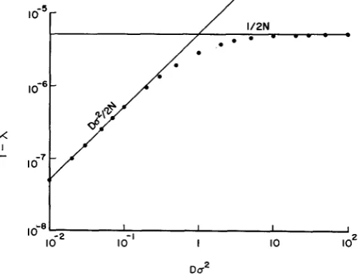
1 ( 4 3 )

Formulae (4-2) and (4-3) hold also with f ( 5 , y ) given in (3-7) with L, = L, and ul2 = u ~ ~ . Transition from formula (4-2) to (4-3) occurs at Da2 = 1 . This is illustrated in Figure 1. The rate given in (4-3) is equal to that of a panmictic population of the same size. I t is interesting to note that if Duz

>

10 the popula- tion behaves nearly as a panmictic population and this is independent of the habitat size. This is in strong contrast to the situation in one-dimensional cases.

la8' I I I I

lo-' I IO IO2

Du2

FIGURE 1.-Relationship between the asymptotic rate (1

-

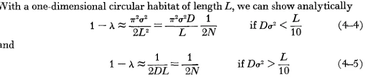
A ) of decrease of genetic varia- bility and Do,, where D =population density and u2 = variance of dispersion distance. Two lines indicate the approximations given by (4-2) and (4-3), while the dots indicate the value of 1 - A obtained from ( 4 1 ) . The values of parameters are L (habitat size) = L , = L, = 100,

With a one-dimensional circular habitat of length L, we can show analytically (4-4) P~U' - i?u'D 1 1

1.-AZ---- if

DO'

<

-

2LZ L 2N 10

and

L

if Do2

> -

10 (4-5

1

(cf. MARUYAMA, 1971,20 in the paper corresponds to U' of the above formulae).

The rate given in (4-5) is equal to that of a panmictic population of size D L .

Therefore, with a one-dimensional population whether it behaves like a panmictic population or not depends on both DO' and L, and, for a fixed Du', as L becomes large it always deviates from a random mating population.

A few examples illustrating these facts are given in Table 1 . In the table, in order to illustrate the validity of the approach taken in this paper, the rates of decay with one-dimensional cases are given by two-different ways, (4-1) and

(4-4) or (4-5). The rates determined by the two different ways agree remark-

TABLE 1

Examples of the asymptotic rate of decrease of genetic variability ( I

-

A) obtained from formula (4-1)

Case 1 2 3 4 5 6 7 8 9 10 11 12 13 14 15 16 17 18 19 20

4 x L*

100

x

100 500 x 500 100

x

100 IOOX 100 500 x 500 100 x 100 5000 x 5000

100 x 100 100

x

100 500 x 500 5000

x

5000

100 100 100 100 100 100 100 500 1 or

L D Do2

1

-

fo u+o 1-7

lim

-

Exact value from

1

-

X MARUYAMA (1971) 1 0.001

10 0.03 10 0.1 10 0.2 10 0.2 1000 2.0 100 2.0 IO 5.0 100 10.0 10 10.0 10 10.0 1 2.0 1 2.0 1 2.0 1 2.0 1 2.0 1 2.0 1 2.0 10 10.0 15 0.03

0.0011 0.0295 0.1012 0.2050 0.1919 0.7134 0.6873 0.8904 0.9308 0.9250 0.9004.

0.7139 ( U = 10-1) 0.4274 ( U = le2) 0.2485 (U = l 0-3)

0.2069 ( U = le4)

0.2014 (U = 10-6)

0.1972 0.2976

0.2020 ( U = 10-5)

0.2004 ( U = 10-7)

5.50 x le8 5.89 X le9

5.06 x 1 0 - 7

1.03 X le6 3.84

x

10-8 3.57 x 10-8 1.38

x

10-IO 4.45

x

10-6 4.65

x

10-7 1.85 X le7 1.80

x

10-9 3.5699

x

10-3 2.1371 X

1.2429 X lk3 1.0346 x 10-3 1.0099 x 1 0 - 3

1.0069 x 10-3

1.0021 x 10-3 1.00

x

10-3

1.97

x

10-5 2.00 x 10-5 9.92

x

10-3 1.00 x 10-2

Cases 1-11 are two dimensional examples, and caws 12-20 are one-dimensional. Li in cases 1-1 1 indicates the length of torus-like habitat along the ith coordinate axis and L in cases 12-20 indicates the length of the circular habitat. D = the number of individuals in unit length or in unit area of the habitat. 'U = the variance of dispersion distance. Cases 12-18 are to show that

formula (4-1) converges to the correct value of 1 - X when U is sufficiently small, ( U = mutation rate). In cases 18-20, the exact value of 1 - h obtained from the iteration method of MARWAMA

GENETIC VARIABILITY 649 ably well, (cases 18

-

20). It has been shown that the rates given in (4-4) or (4-5) agree well with the exact value obtained by a direct method of numerical iteration, (cf. MARUYAMA, 1971).

With a population occupying a plane rectangular habitat of size L X L, nu- merical calculations show that the formulae corresponding to (4-2) and (4-3) are

(4-2’)

U2

4L2

l - A Z - if

D 2

<

2 and

1 l - A Z -

2DL2 if Du2

>

2 (4-3’)

respectively. And with a linear population of length L and with two ends, the corresponding formulae to (4-4) and (4-5) are

and

L

if Do2

> -

1 - 1

l - A Z - - -

2DL 2N 5 - (4-5’)

These approximations can be obtained analytically, (cf. MARUYAMA 1971 )

.

We note that there is no essential difference between circular and linear populations, and between torus-like and rectangular populations.

5.

EIGENFUNCTION

In addition to the rate of decay discussed in the previous section, the shape of the function h ( t , z, y ) is of considerable importance, because it gives information on the dfferentiation of the local gene frequencies. Let

h ( x , y )

=

lim c(1 - f ( x , y ) ) U” 0

in which f (2, y ) is given in ( 3 - 3 ) and c is a normalization constant. If f ( 0 , 0 ) J

f (L,/2, L , / 2 ) =: 0, the local differentiation is strong, and if the ratio is nearly unity, the population is approximately panmictic. With a one-dimensional popu- lation,

h ( s )

=

lim c ( 1 - f ( x ) ) (5-2) u+o

where f ( x ) is given in (3-9). It is known that h ( s ) cc sims/L, if Do2 L, and

furthermore we can calculate the exact values of h ( x ) by a direct method of

numerical iteration, (cf. MARUYAMA 1971). In order to illustrate the validity of (5-1 )

,

using one dimensional examples, the values obtained by the three methods are compared in Table 2.

TABLE 2

Comparison of the function given by (5-2) and the eigenfunction obtained by the iteration melhod of MARUYAMA (1971 )

Example 1 Example 2

-

X sin

(g)

L from (5-2) from iteration from (5-2) from iteration

0 0.05 0.10 0.15 0.20 0.25 0.30 0.35 0.40 0 . 6 0.50 0.0175 0.0333 0.0540 0.0724 0.0884 0.1022 0.1126 0.1217 0.1295 0.1330 0.1352 0.01 72 0.0323 0.0516 0.0698 0.0865 0.1012 0.1138 0.1238 0.1311 0.1356 0.1371 0.01 80 0.0329 0.0535 0.0723 0.0886 0.1023 0.1136 0.1223 0.1295 0.1333 0.1336 0,0184 0.0339 0.0516 0.0696 0.0860 0.1001 0.1133 0.1233 0.1306 0.1351 0.1366 0 0.0228 0.0451 0.0662 0.0858 0.1032 0.1181 0.1300 0.1388 0,1441 0.1469

The values of the parameters in example 1 are L = 100, D = 1, ~2 = 1; the parameters in

example 2 are L = 1, D = 10, 02 = 0.002. Function h ( z ) gives the asymptotic form of relative

heterozygosity in the habitat.

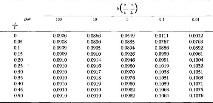
contrary. This view is illustrated in Table 3 by comparing several cases of the diagonal elements of function h ( z , y), i.e.,

x

= y.

TABLE 3

Numerical examples of the values of the function h ( x , y) of (5-1)

Do2 100 10 1 0.1 0.01

X - L 0 0.05 0.1 0.15 0.20 0.25 0.30 0.35 0.40 0.45 0.50 0.0906 0.0908 0.0909 0.0909 0.0910 0.0910 0.0910 0.0910 0.0910 0.0910 0.0910 0.0866 0.0896 0.0905 0.0910 0.0914 0.0916 0.0917 0.0918 0.0919 0.0919 0.0919 0.0549 0.0835 0.0894 0.0926 0.09% 0.0960 0.0970 0.0976 0.0980 0.0982 0.0982 0.0111 0.0767 0.0886 0.0950 0.0991 0.1019 0.1038 0.1051 0,1059 0.1063 0.1064 0.0012 0.0763 0.0892 0.0961 0 . 1 m 0.1 032 0.1051 0.1063 0.1071 0.1075 0.1076

GENETIC VARIABILITY

65

1

I would like to thank Dr. M o ~ o o KIMURA who directed my attention to the subjects of this

paper and for the encouragement and help he has offered at all times, and the referees for many useful criticisms and comments.

LITERATURE CITED

BODMER, W. F. and L. L. CAVALLI-SFORZA, 1968

FISHER, R. A., 1922

H.~RRIS, H., 1966

KIMURA, M. and T. OHTA, 1971 Protein polymorphism as a phase of molecular evolution. Na- ture 229: 467-469.

KIMURA, M. and G. H. WEISS, 1964. The stepping stone model of population structure and the decrease of genetic correlation with distance. Genetics 49: 461-576.

LEWONTIN, R. C. and J. L. HUBBY, 1966 A molecular approach to the study of genic heterozy- gosity in natural populations. 11. Amount of variation and degree of heterozygosity in nat- ural populations of Drosophila pseudoobscura. Genetics 54: 595-609.

MAL~COT, G., 1948 Les mthe‘matiques de Z’hbridite. Mason et Cie, Paris. -, 1950 Quelques schemas probabilistes sur la variabilit6 des populations naturelles. Ann. Univ. Lyon, Sciences, Section A 13: 37-60. -, 1951 Un traitement stochastique des prob- 16mes lin6aires (mutation, linkage, migration) en g6nGtique de populations. Ann. Univ. Lyon, Science, Section A 14: 79-117.

-,

1962 Migration et parent6 g6n6tique moy- enne. pp. 205-212. In: Entretiens de I\.lonaco en sciences humaines. - , 1967 Identical loci and relationship. Proc. 5th Berkeley Symp. Math. Stat. Prob. 4: 31 7-332.

The rate of decrease of heterozygosity in a population occupying a cir- cular or a linear habitat. Genetics 67: 437-464.

The effect of nonrandom mating within inbred lines on the rate of in- breeding. Genetical Research 5: 164-167.

Eigenfunction expansions associated with second-order differential equations. Part two, first edition. Clarendon press, Oxford.

Isolation by distance. Genetics 23: 114-138. -, 1 9 G Isolation by distance under di- verse systems of mating. Genetics 31 : 39-59. The genetical structure of pop- ulations. Ann. Eugenics 15: 323-354.

A migration matrix model for the study of

1930 random genetic drift. Genetics 59: 565-592.

The distribution of gene ratios for rare mutations. Proc. Roy, SOC. Edinb. 50: 205-220. On the dominance ratio. Proc. Roy. Soc. Edinb. 42: 321-341.

Enzyme polymorphism in man. Proc. Roy. Soc. B. 1\64: 298-310.

- ,

MARUYAMA, T., 1971

ROBERTSON, A., 1964

TITCHMARSH, E. C., 1958

WRIGHT, S., 1931 Evolution in Mendelian populations. Genetics 16: 97-159.

-

, 1943