Updated Ground Motion Models For AI And CAV Using The NGA-West2 Database

(1)

Transactions, SMiRT-25 Charlotte, NC, USA, August 4-9, 2019

Division IV

UPDATED GMPES FOR AI AND CAV USING THE

NGA-WEST2 DATABASE

Kenneth W. Campbell1, Yousef Bozorgnia2

1

Principal, Science & Analytics, CoreLogic, Inc., Oakland, CA, USA ([email protected]) 2

Professor, Department of Civil and Environmental Engineering, UCLA, Los Angeles, CA, USA

ABSTRACT

We have updated our NGA-West1 ground motion prediction equations (GMPEs) for the horizontal components of Arias intensity (AI) and cumulative absolute velocity (CAV) using the much larger West2 database. We use the same database and functional form we used to develop GMPEs for our NGA-West2 ground motion intensity measures (GMIMs). Our results show that the NGA-NGA-West2 functional form can be used to model AI and CAV. Our results also show that CAV has the best goodness-of-fit statistics of all the GMIMs we have evaluated up to this time. Its relatively small between-event and within-event standard deviations confirm its superior predictability. On the other hand, AI has the highest standard deviation of any GMIM we have studied thus far, which is approximately double that of CAV and substantially larger than those of peak-amplitude and spectral GMIMs, resulting in relatively low predictability. Thus, CAV may be considered a preferred choice for some applications in the context of performance-based earthquake engineering depending on the structural or geotechnical engineering demand parameters of interest.

INTRODUCTION

In this study, we updated our horizontal GMPEs (or ground motion models, GMMs) for AI and CAV using the same subset of the NGA-West2 ground motion database (Ancheta et al. 2014) and functional form that we used to develop GMPEs for the horizontal and vertical components of peak ground acceleration (PGA), peak ground velocity (PGV), and peak 5%-damped pseudo-spectral acceleration (PSA) (Campbell and Bozorgnia 2014; Bozorgnia and Campbell 2016a,b).

The mathematical definitions of AI and CAV are given by the following equations (Arias 1970; EPRI 1988; Reed and Kassawara 1990):

2 0

AI ( )

2

max

t

a t dt g

π

=

∫

(1)

0

CAV=

∫

tmax a t dt( ) (2)

where g is the gravitational constant (9.81 m/s2), ( )a t is the amplitude of the acceleration time series at

(2)

BACKGROUND

In a previous study, we developed GMPEs for CAV (CB10; Campbell and Bozorgnia 2010) and AI (CB12; Campbell and Bozorgnia 2012) using the same subset of the PEER NGA-West1 ground motion database (Chiou et al. 2008) and the same functional form used to develop GMPEs for the horizontal components of PGA, PGV, and PSA (Campbell and Bozorgnia 2008), inelastic PSA (Bozorgnia et al. 2010), and Japan Meteorological Agency (JMA) instrumental seismic intensity (Campbell and Bozorgnia 2011). We refer the reader to these publications for a review of other studies of CAV and AI that were available up to that time.

AI has traditionally been used to assess the impact of ground shaking on slope stability (Jibson 2011) and there are several recent studies that continue to support this tradition using statistical correlations between AI and engineering demand parameters (EDPs) related to earthquake-induced slope failure. Since Kramer and Mitchel (2006) first concluded that CAV was optimally correlated with excess pore pressure generation in potentially liquefiable soils, recent studies have confirmed and supported this tradition using statistical correlations between CAV and many soil liquefaction and settlement-based EDPs, although a few studies have shown that AI rather than CAV correlates better with some liquefaction EDPs.

Since our previous studies were completed, several investigators have developed GMPEs for AI and CAV from a variety of global, regional, and country-specific databases from active shallow tectonic environments. Because of length restrictions, it is not possible to review all of these GMPEs or show how they compare with those developed in this study. We do, however, compare our new GMPEs with those we developed previously using the NGA-West1 database.

GROUND MOTION DATABASE

The database used in this study is the same subset of the PEER NGA-West2 ground motion database (Anchetta et al. 2014) used to develop our NGA-West2 empirical GMPEs for the horizontal and vertical components of PGA, PGV, and PSA (Campbell and Bozorgnia 2014; Bozorgnia and Campbell, 2016a,b).

The selected database consists of 15,521 recordings from 322 earthquakes with 3.0≤M≤7.9. The

database includes 7,208 near-source recordings (R_RUP ≤80 km) from 282 worldwide earthquakes and

8,313 far-source recordings (80<R_RUP ≤500 km) from 276 worldwide earthquakes. Many of these

earthquakes have recordings from both databases. The reader is referred to Campbell and Bozorgnia (2014) [CB14] and Campbell and Bozorgnia (2019) [CB19) for additional details including the definition of all of the predictor variables and a figure showing the distribution of the recordings with respect to magnitude and distance.

The predictor variables used in the GMMs are defined as follows: M is the moment magnitude;

RUP

R (km) is closest distance to the coseismic rupture surface (a.k.a. rupture distance); R_JB (km) is closest distance to the surface projection of the coseismic rupture surface (a.k.a. Joyner-Boore distance);

X

R (km) is closest perpendicular distance to either the surface projection of the top edge of the coseismic

rupture surface or its extension off the ends of the rupture parallel to the average strike angle (R_X is positive when on the hanging-wall side and negative when on the footwall side of the coseismic rupture surface); W (km) is average down-dip width of the coseismic rupture surface; λ (°) is average rake angle defined as the average angle of slip measured in the plane of rupture between the average strike direction and the slip vector; F_RV is an indicator variable for reverse and reverse-oblique faulting: F_RV =1 for

(3)

faulting: F_NM =1 for −150° < < − °λ 30 and F_NM =0 otherwise; Z_TOR (km) is average depth to the top of the coseismic rupture surface; δ (°) is average dip angle of the coseismic rupture surface relative to a horizontal plane; VS30 (m/s) is time-averaged shear-wave velocity in the top 30 m of the site (a.k.a. site

velocity); A1100 (g) is predicted median value of PGA on a rock outcrop with VS30 =1100 m/s (a.k.a. rock

PGA); Z2.5 (km) is depth to the 2.5 km/s shear-wave velocity horizon beneath the site (a.k.a. sediment

depth or basin depth); and Z_HYP (km) is hypocentral depth.

GROUND MOTION PREDICTION EQUATIONS

The natural logarithm of the horizontal components of the GMIMs of interest in this study are represented by the following generalized GMPE:

lnY = f_mag+ f_dis+ f_flt+ f_hng + f_site + f_sed + f_hyp + f_dip + f_atn + +η ε_i _ij (3)

where Y is the GMIM of interest and the f-terms represent the scaling of Y (actually lnY , the natural log of Y), with terms representing earthquake magnitude, geometric attenuation, style of faulting, hanging-wall geometry, shallow site response, deep sedimentary (basin) response, hypocentral depth, fault dip angle, and anelastic attenuation, respectively. The independent normally distributed variables η_i and ε_ij

have zero means and estimated between-event and within-event standard deviations on reference rock with V_S₃₀=1100 m/s and softer sites exhibiting linear site response of τ_ln_Y and φ_ln_Y. The mathematical representation of the terms in equation 3 are defined in CB14. The model coefficients and the between-event and within-between-event standard deviations of the GMPEs for each GMIM were determined using the

NLME nonlinear mixed-effects regression package in the R statistical software platform (Pinheiro et al. 2017).

The standard deviations τ_ln_Y and φ_ln_Y were found to be magnitude dependent with coefficients τ₁,

2

τ , φ₁, and φ₂ (see equation in CB14). Other parameters that are necessary to calculate the final aleatory standard deviations τ and

φ

, including their dependence on nonlinear site effects, are φ_ln_AF, the

estimated standard deviation of fsite for linear site response, ρlnPGA,lnY, the correlation coefficient between

the natural logarithm within-event residuals of the GMIM and PGA, and α, the linearized functional

relationship between f_site and lnA₁₁₀₀. The reader is referred to CB14 for the equations needed to estimate these aleatory parameters.

The model coefficients included in the GMPEs are c₀−c₂₀, ∆c20, c, n, k1−k3, a2, and h1−h6

(CB14). The c_i and ∆c20 coefficients were determined from the regression analyses in which the

coefficient ∆c₂₀ accounts for regional differences in anelastic attenuation for those regions where sufficient data are available to determine a separate anelastic attenuation coefficient. The base region used to derive c₂₀ includes California, Taiwan, the Middle East and similar active tectonic regions for which

we set ∆c₂₀ =0. The regions used to derive non-zero values of ∆c₂₀ include Japan and Italy (∆c_20,JI),

representing relatively higher anelastic attenuation regions, and eastern China (∆c_20,CH), representing

(4)

attenuation term was regionally independent. The coefficients c, n, and k₁−k₃ are related to the shallow

site and basin terms and the coefficients h₁−h₆ are related to the hanging-wall term. These coefficients were constrained from theoretical and numerical studies as described in CB14. The nonlinear mixed-effects regression coefficients and aleatory goodness-of-fit measures are summarized in Table 1.

MODEL PREDICTIONS

Figure 1 shows how the median predicted values of the GMIMs scale with M and

R

_X for

V

_S₃₀

=

760

m/s and default values of

Z

_HYP,

Z

_TOR, and

Z

_2.5 calculated from relationships given in CB14. The distance metric

R

_X is used for these plots because it is a convenient measure for comparing GMMs. These default values are used for all subsequent plots except where noted. The solid lines correspond to a vertical strike-slip earthquake and the dashed lines to a 45°-dipping reverse-faulting earthquake along a hanging-wall distance profile that is perpendicular to the top edge of the center of the fault. This figure clearly shows the strong hanging-wall effects exhibited by both GMIMs at large magnitudes and short distances. This

figure also shows the stronger magnitude and distance scaling of

AI

_GM compared to

CAV

_GM after

accounting for the change in scales of the ordinate.

Figure 2 shows the median predicted site-amplification factors for shallow site response (V_S₃₀

term) and basin response (Z_2.5 term) for a vertical strike-slip earthquake with R_RUP =10 km and M=4.0, 5.0, 6.0, 7.0, and 8.0. Linear shallow site response scaling is indicated by all the curves plotting on top of each other. The departure from linear scaling is indicated by the separation of the curves at V_S₃₀<400 m/s. Basin response is independent of magnitude which is why there is a single set of curves for each GMIM. The stronger scaling exhibited by AI_GM is directly related to its definition in terms of the square of acceleration.

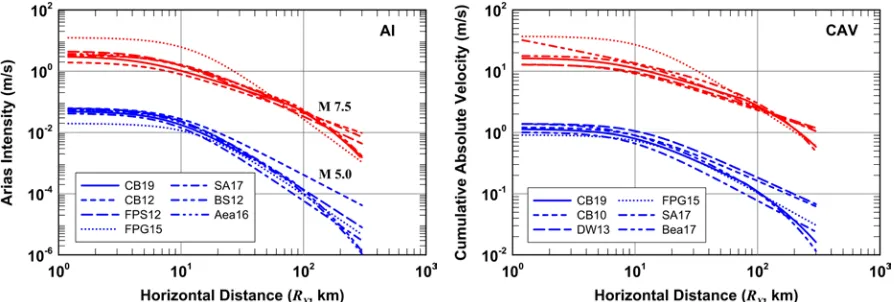
Figure 3 compares the attenuation characteristics of the median predicted values of the GMIMs

from CB19 with our previous GMMs for CAV_GM (CB10) and AI_GM (CB12) and with other GMMs

recently published in the literature, namely Du and Wang (2013) [DW13], Foulser-Piggott and Goda

(2015) [FPG15], Sandikkaya and Akkar (2017) [SA17], and Bullock et al. (2017) [Bea17] for CAV_GM

and FPG15, SA17, Foulser-Piggott and Stafford (2012) [FPS12], Bustos and Stafford (2012) [BS12], and

Abrahamson et al. (2016) [Aea16] for AI_GM. These last two GMMs require median estimates of PGA_GM

and PSAGM(T =1 s) which we estimate from CB14 for consistency with CB19 that was developed using

the same database as CB14. The comparison is for a vertical strike-slip earthquake, M=5.0 and 7.5, and

30 760

S

V = m/s. We generally do not recommend comparing country-specific GMMs with pan-regional

(5)

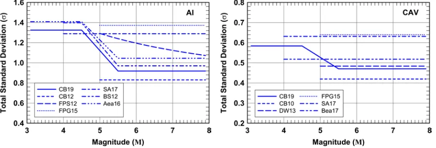
Figure 4 compares the total standard deviations from CB19 and the same GMMs evaluated in Figure 3 plotted against magnitude. The ranges of values are limited to those recommended by the developers. The plots assumed linear site response for those standard deviations that are a function of V_S₃₀

or site class (i.e., those that include a nonlinear site response term), which include all but SA17 and Bea17, the latter because it includes only rock sites. BS12 and Aea16 include nonlinear site effects and magnitude-dependence imputed from the standard deviations of CB14 for PGA_GM and PSA_GM(T =1 s). There are two notable observations from Figure 4: (1) there is a wide spread of standard deviations among

the various models and (2) those studies that developed GMMs for both AI_GM and CAV_GM using the

same database and functional form show that the latter has standard deviations approximately half those of the former due to the former’s definition as the integral of the square of acceleration.

CONCLUSIONS

Since we used the same database and functional form as CB14, we refer the reader to this latter publication for a description of the ranges of applicability and for guidance on the use of the GMMs presented in this paper. For example, the evaluation of the nonlinear part of the site term ( fsite) and the

within-event standard deviation (φ) requires an estimate of rock PGA (A₁₁₀₀) from CB14. One of the more significant results of this study is the superior goodness-of-fit measures of the predicted value of

GM

CAV as indicated by comparing standard deviations and coefficients of determination in Table 1. Like

in our previous models (CB10 and CB12), we find these measures to be superior to those for the predicted

values of AI_GM and, for that matter, any of the horizontal peak-amplitude GMIMs from GMMs that was

developed using the same database and functional form (CB14; Bozorgnia and Campbell 2016b). Additional details can be found in Campbell and Bozorgnia (2019).

Consistent with CB12, our current results show that the natural logarithmic standard deviations of

GM

AI are about two times higher than that of CAV_GM (Table 1). This result is also consistent with other studies that have evaluated these GMIMs using the same database and functional form (e.g., Kramer and Mitchell 2006; Danciu and Tselentis 2007; FPG15; Bea17; SA17). This result is directly related to the definition of AI as proportional to the square rather than the absolute value of acceleration, which corresponds to a factor of two increase in the residuals and resulting standard deviations. We find that the marginal and conditional coefficients of determination (

R

m2 and

2

c

R

) of the CAV_GM GMM are also higher

than those of the AI_GM GMM. The goodness-of-fit values LL, AIC, BIC, DIC cannot be directly

compared because of the difference in the GMIM definitions, even though they have the same units and were developed using the same database and functional forms. However, the values of these statistics can

be compared if the values for AI_GM are divided by two, owing to their dependence on the square of

acceleration. In this case, the CAV_GM GMM has lower values of AIC, BIC, and DIC and a higher value of LL, indicating a better fit to the data. These results together with the smaller standard deviations indicate that CAV_GM has a higher level of predictability than AI_GM. The goodness-of-fit statistics in Table 1 also

indicate that CAV_GM is more predictable than PGA_GM and, although not shown, than PGV_GM or

( ) GM

(6)

REFERENCES

Abrahamson, C., Shi, H.-J. M., and Yang, B. (2016). Ground-Motion Prediction Equations for Arias

Intensity Consistent with the NGA-West2 Ground-Motion Models, PEER Report 2016/05, Pacific Earthquake Engineering Research Center, University of California, Berkeley, 42 pp.

Ancheta, T. D., Darragh, R. B., Stewart, J. P., Seyhan, E., Silva, W. J., Chiou, B. S.-J., Wooddell, K. E., Graves, R. W., Kottke, A. R., Boore, D. M., Kishida, T., and Donahue, J. L. (2014). “PEER NGA-West2 Database,” Earthq. Spectra, 30, 989–1005.

Arias, A., 1970. “A Measure of Earthquake Intensity,” in Seismic Design for Nuclear Power Plants, R. J. Hansen (ed.), The MIT Press, Cambridge, MA, 438–483.

Bozorgnia, Y., and Campbell, K. W. (2016a). “NGA-West2 Ground Motion Model for the

Vertical-to-Horizontal Ratio of PGA, PGV, and Linear Response Spectra,” Earthq. Spectra, 32, 951–978.

Bozorgnia, Y., and Campbell, K. W. (2016b). “Vertical Ground Motion Model for PGA, PGV, and

Linear Response Spectra Using the NGA-West2 Database,” Earthq. Spectra, 32, 979–1004.

Bozorgnia, Y., Hachem, M. M., and Campbell, K. W. (2010). “Ground motion Prediction Equation (“Attenuation” Relationship”) for Inelastic Response Spectra,” Earthq. Spectra, 26, 1–23.

Bullock, Z., Dashti, S., Liel, A., Porter, K., Karimi, Z., and Bradley, B. (2017). “Ground-motion Prediction Equations for Arias Intensity, Cumulative Absolute Velocity, and Peak Incremental Ground Velocity for Rock Sites in Different Tectonic Environments,” Bull. Seismol. Soc. Am., doi: 10.1785/0120160388.

Bustos, A. G., and Stafford, P. J. (2012). “On the Use of Arias Intensity as a Lower Bound in the Hazard

Integration Process of a PSHA,” Proc., 15th World Conference on Earthquake Engineering,

Lisbon, Portugal, 12, 9011–9020.

Campbell, K. W. (2018). “Engineering Models of Strong Ground Motion,” in Earthquake Engineering

Handbook, 2nd ed., Chen, W. F., and Scawthorn, C. (eds.), CRC Press, Boca Raton, FL, Chapter 5, in press.

Campbell, K. W., and Bozorgnia, Y. (2008). “NGA Ground Motion Model for the Geometric Mean Horizontal Component of PGA, PGV, PGD and 5% Damped Linear Elastic Response Spectra for Periods Ranging from 0.01 to 10 s,” Earthq. Spectra, 24, 139–171.

Campbell, K. W., and Bozorgnia, Y. (2010). “A Ground Motion Prediction Equation for the Horizontal

Component of Cumulative Absolute Velocity (CAV) Using the PEER-NGA Database,” Earthq.

Spectra, 26, 635–650.

Campbell, K. W., and Bozorgnia, Y. (2011). “A Ground Motion Prediction Equation for JMA Instrumental Seismic Intensity for Shallow Crustal Earthquakes in Active Tectonic Regimes,”

Earthq. Eng. Struct. Dyn., 40, 413–427.

Campbell, K. W., and Bozorgnia, Y. (2012). “A Comparison of Ground Motion Prediction Equations for Arias Intensity and Cumulative Absolute Velocity Developed Using a Consistent Database and Functional Form,” Earthq. Spectra, 28, 931–941.

Campbell, K.W., and Bozorgnia, Y. (2014). “NGA-West2 Ground Motion Model for the Average Horizontal Components of PGA, PGV, and 5%-damped Linear Acceleration Response Spectra,”

Earthq. Spectra, 30, 1087–1115.

Campbell, K.W., and Bozorgnia, Y. (2019). “Ground Motion Models for the Horizontal Components of Arias Intensity (AI) and Cumulative Absolute Velocity (CAV) Using the NGA-West2 Database,”

Earthq. Spectra, 35, in press.

Chiou, B., Darragh, R., Gregor, N., and Silva, W. (2008). “NGA Project Strong-Motion Database,”

Earthq. Spectra, 24, 23–44.

Danciu, L., and Tselentis, G. (2007). “Engineering Ground-motion Parameters Attenuation Relationships for Greece,” Bull. Seismol. Soc. Am., 97, 162–183.

(7)

EPRI (1988). A Criterion for Determining Exceedance of the Operating Basis Earthquake, Report EPRI NP-5930, Electric Power Research Institute, Palo Alto, CA, 330 pp.

Foulser-Piggott, R., and Goda, K. (2015). “Ground-motion Prediction Models for Arias Intensity and Cumulative Absolute Velocity for Japanese Earthquakes Considering Single-station Sigma and Within-event Spatial Correlation,” Bull. Seismol. Soc. Am., 105, 1903–1918.

Foulser-Piggott, R., and Stafford, P. J. (2012). “A Predictive Model for Arias Intensity at Multiple Sites and Consideration of Spatial Correlations,” Earthq. Eng. Struct. Dyn., 41, 431–451.

Jibson, R. W. (2011). “Methods for Assessing the Stability of Slopes During Earthquakes—A Retrospective,” Eng. Geol., 122, 43–50.

Kramer, S. L., and Mitchell, R. A. (2006). “Ground Motion Intensity Measures for liquefaction Hazard Evaluation,” Earthq. Spectra, 22, 413–438.

Reed, J. W., and Kassawara, R. P. (1990). “A Criterion for Determining Exceedance of the Operating Basis Earthquake,” Nucl. Eng. Des., 123, 387–396.

Sandikkaya, M. A., and Akkar, S. (2017). Cumulative Absolute Velocity, Arias Intensity and Significant

Duration Predictive Models from A Pan-European Strong-Motion Dataset, Bull. Earthq. Eng., 15,

1881–1898.

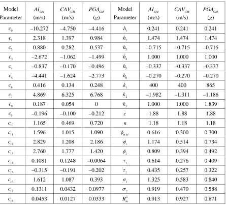
Table 1: Summary of regression coefficients and goodness-of-fit parameters.

Model Parameter GM AI (m/s) GM CAV (m/s) GM PGA

(g)

Model Parameter GM AI (m/s) GM CAV (m/s) GM PGA

(g)

0

c –10.272 –4.750 –4.416 h1 0.241 0.241 0.241

1

c 2.318 1.397 0.984 h2 1.474 1.474 1.474

2

c 0.880 0.282 0.537 h3 –0.715 –0.715 –0.715

3

c –2.672 –1.062 –1.499 h4 1.000 1.000 1.000

4

c –0.837 –0.170 –0.496 h5 –0.337 –0.337 –0.337

5

c –4.441 –1.624 –2.773 h6 –0.270 –0.270 –0.270

6

c 0.416 0.134 0.248 k1 400 400 865

7

c 4.869 6.325 6.768 k2 –1.982 –1.311 –1.186

8

c 0.187 0.054 0 k3 1.000 1.000 1.839

9

c –0.196 –0.100 –0.212 c 1.88 1.88 1.88

10

c 1.165 0.469 0.720 n 1.18 1.18 1.18

11

c 1.596 1.015 1.090 φlnAF 0.616 0.300 0.300

12

c 2.829 1.208 2.186 φ1 1.174 0.514 0.734

13

c 2.760 1.777 1.420 φ2 0.809 0.394 0.492

14

c 0.1081 0.1248 –0.0064 τ1 0.614 0.276 0.409

15

c –0.315 –0.191 –0.202 τ2 0.435 0.257 0.322

16

c 1.612 1.087 0.393 σ1 1.325 0.583 0.840

17

c 0.1311 0.0432 0.0977 σ2 0.919 0.470 0.588

18

(8)

19

c 0.01242 0.00429 0.00757 R_c2 0.936 0.948 0.903

20

c –0.0103 –0.0043 –0.0055 LL –11,232 –5,382.0 –7,621

20,JI c

∆ –0.0051 –0.0024 –0.0035 AIC 22,505 10,806 15,284

20,CH c

∆ 0.0064 0.0027 0.0036 BIC 22,650 10,950 15,429

1

a 0.167 0.167 0.167 DIC 22,463 10,764 15,242

Note: All standard deviations are in natural log units and represent linear site conditions.

Figure 1: Scaling of AI_GM (left column) and CAV_GM (right column) with R_X (top row) and M (bottom

(9)

Figure 2: Scaling of median predicted site-amplification factors for AI_GM (solid lines) and CAV_GM

(dashed lines) with V_S₃₀ (left plot) and Z_2.5 (right plot) for a vertical strike-slip earthquake with R_RUP =10

km and M=4.0−8.0.

(10)