Theses and Dissertations
12-14-2015
Optimized Spectral Processing of Infrared Diffuse
Reflection Spectra for the Detection of Blood on
Fabric
Stephanie Ann DeJong
University of South Carolina - Columbia
Follow this and additional works at:https://scholarcommons.sc.edu/etd Part of theChemistry Commons
This Open Access Dissertation is brought to you by Scholar Commons. It has been accepted for inclusion in Theses and Dissertations by an authorized administrator of Scholar Commons. For more information, please [email protected].
Recommended Citation
by
Stephanie Ann DeJong
Bachelor of Arts
Trinity Christian College, 2011
Submitted in Partial Fulfillment of the Requirements
For the Degree of Doctor of Philosophy in
Chemistry
College of Arts and Sciences
University of South Carolina
2015
Accepted by:
Michael L. Myrick, Major Professor
S. Michael Angel, Committee Chair
Stephen L. Morgan, Committee Member
John W. Weidner, Committee Member
and enabled me to be successful in my pursuit of this degree. First, I would like
to thank my committee members Dr. Angel, Dr. Weidner, and Dr. Morgan, whose
advice and guidance over the past few years has been greatly appreciated. I
particularly thank Dr. Morgan, who continually encouraged me to carefully
consider both my words and my data, because I should be ready to defend either
at all times. I would also like to thank Dr. Lou Sytsma, my undergraduate
research advisor, without whose encouragement I might not have decided to
attend graduate school.
I am also much obliged to my fellow Myrick lab members: Dr. Joe
Swanstrom, for introducing me to the lab and grad school; Elizabeth Abernathy,
for always being willing to help; Shawna Tazik, who has been with me at every
step along this journey; Brianna Cassidy and Zhenyu Lu, honorary Myrick lab
members; and to Cameron Rekully, Ray Belliveau, and Stefan Faulkner for all
their engaging conversations.
I could not have accomplished any of what I’ve done without the
continuing love and support of my parents, Charles and Monique DeJong. They
I may not have known I would be working with him when I arrived at U.S.C., but I
now sincerely feel that my graduate experience would not have been nearly as
fulfilling with any other advisor. There are few people I respect as much both
personally and professionally. Dr. Myrick has seen me at some of my best and
some of my worst moments, but his kindness rarely flagged; his response was
almost always: “Let’s get coffee.” So thank you for all the coffee, tea, support,
important to the forensic community. Luminol, which participates in a
chemiluminescent reaction with the heme groups of blood, is one of the most
commonly used presumptive tests. Luminol has a few drawbacks, including the
requirement of use in a dark environment and potential to degrade the amount of
recoverable DNA in blood stains. A potential complementary method is infrared
(IR) spectroscopy. These two methods are compared in this work.
Infrared diffuse reflection (DR) spectroscopy works well to measure the IR
spectrum of samples that are highly absorbing or scattering, such as fabric. In
the IR DR spectrum of blood on fabric, the contribution of analyte signal to the
total signal is weak, and many of the characteristic amide absorbance bands of
blood proteins overlap with the spectral features of fabrics. Derivative
transformations are commonly applied to resolve overlapping spectral peaks.
These transformations are typically implemented as Savitzky-Golay (SG)
derivatives. The performance of optimized higher-order gap derivatives (GDs)
and SG derivatives are compared here as preprocessing methods for partial
least-squares regression (PLSR), a multivariate calibration technique. Optimized
to examine the RVs in the original spectral space, which is more familiar to
spectroscopists. To that end, we offer a method of calculating higher-order GDs
that allows the resulting GD and RVs to be exactly integrated to spectral space.
Infrared detection limits (DLs) for blood on four fabric types (acrylic,
cotton, nylon, and polyester) were estimated using optimized GD processing and
PLSR. The best IR DLs for blood on fabric were found in the mid-IR spectral
region. The DLs for acrylic, cotton, and polyester fabrics were blood diluted by
factors of 2300, 610, and 900, respectively. Due to the similarity between the IR
spectra of blood solids and nylon, no satisfactory IR DLs were determined for the
calibration of blood on nylon. These DLs are on the order of the most commonly
reported DLs (1000x dilute) for blood on fabric using the standard luminol
method. An approach to further improve the DL by accounting for known sources
ABSTRACT ... v
LIST OF TABLES ... x
LIST OF FIGURES ... xi
CHAPTER 1 Introduction ... 1
1.1. Infrared Spectroscopy and Forensic Science ... 1
1.2. Diffuse Reflection Infrared Spectroscopy ... 3
1.3. Multivariate Calibration ... 4
1.4. Dissertation Outline ... 6
REFERENCES ... 9
CHAPTER 2 Influence of Gap Selection on the Performance of Gap Derivatives ... 13
2.1. Introduction ... 13
2.2. Gap Derivative Calculation ... 15
2.3. Influence of Gap Size on Derivative Shape for a Lorentzian Bandshape ... 16
2.4. Influence of Gap Size on SNR for a Lorentzian Bandshape ... 19
2.5. Conclusions ... 26
REFERENCES ... 27
3.4. Conclusions ... 72
REFERENCES ... 74
CHAPTER 4 Reversible Gap Derivatives and Their Integration ... 76
4.1. Introduction ... 76
4.2. Algorithm ... 77
4.3. Experimental ... 95
4.4. Results ... 96
4.5. Conclusions ... 107
REFERENCES ... 108
CHAPTER 5 Detection Limits for Blood on Fabric Using Infrared Diffuse Reflection Spectroscopy ... 109
5.1. Introduction ... 109
5.2. Method ... 112
5.3. Spectral Region Overviews ... 123
5.4. Calibration Results ... 127
5.5. Conclusions ... 138
REFERENCES ... 144
CHAPTER 6 Infrared Camera Used to Measure Electrode Heating During Cyclic Voltammetry ... 149
6.1. Introduction ... 149
6.2. Method ... 151
6.3. Results and Discussion ... 155
6.4. Conclusions and Future Work ... 160
7.2. Looking Forward: Systematic Improvement of Detection Limits ... 164
REFERENCES ... 171
APPENDIX A Reversible Gap Derivative Matlab Code ... 175
of variable != 4!!+1 ... 18
Table 2.2 Maximum values of GDs ... 23
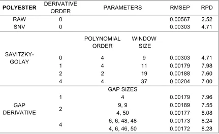
Table 3.1 Parameters of best calibration for blood on polyester in each preprocessing group ... 42
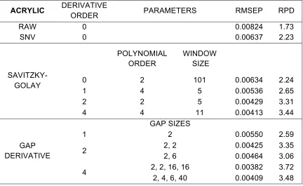
Table 3.2 Parameters of best calibration for blood on acrylic in each preprocessing group ... 43
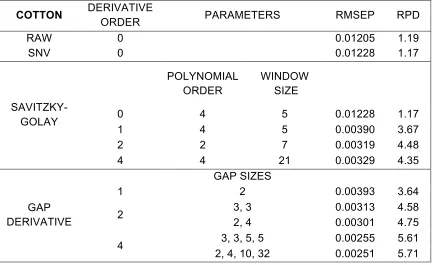
Table 3.3 Parameters of best calibration for blood on cotton in each preprocessing group ... 44
Table 4.1 Example of differentiation and integration for 12-point vector with gap = 4 ... 80
Table 4.2 Data treatments applied after differentiation ... 93
Table 5.1 DLs for blood on fabric in different spectral regions expressed as mass percentage (%w/w), dilution factor, coverage (µg/cm2), and film thickness (nm). ... 132
Table 5.2 DL confirmation results ... 134
Table 5.3 Blood stain area ... 140
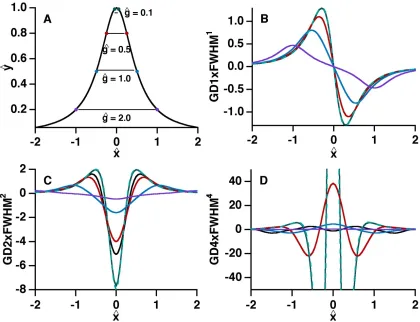
Lorentzian curve (centered at 0) are shown. Each derivative plot shows the AD (dashed line), and GD with ! = 0.1 (dark green), 0.5 (red), 1.0 (blue), and 2.0 (purple). On c-d, the black trace shows the GD calculated with multiple gaps (see text). The GD deviates from the true derivative proportionally to derivative order and gap size. Gap sizes are given in units of FWHM to show the influence of gap size relative to the FWHM of the peak. Each derivative is scaled by the FWHMn. For n = 4, the scale has been adjusted to show the derivative calculated with larger gap sizes. The maximum of GD4 with ! = 0.1is off-scale at approximately 318 units ... 17
Figure 2.2 GD4 of Lorentzian with SNR = 10. (a) The curve from Fig. 2.1a (center at 0, FWHM = 1) with white gaussian noise added. (b) GD4 of (a) with ! = 0.1. The noise is enhanced relative to the signal and completely obscures the peak. (c) GD4 of (a) with ! = 1.0. The signal is now clearly visible above the noise, though the amplitude is much lower ... 21
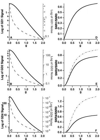
Figure 2.3 SNR of GDs. Panels a/d, b/e, and c/f display information for GD1, GD2, and GD4, respectively, of the Lorentzian curve in Fig. 2.2a. The left column shows the change in signal (solid) and noise (dashed) of the GD as a function of !. With increasing ! at all n, the magnitude of both the signal and the noise decreases, though the noise decreases more rapidly. The right column displays relative SNRn (SNR of GDn divided by SNR of the original curve) as a function of !. For all n, SNRn/SNR0 increases rapidly as ! approaches 1, then begins to plateau. The dashed trace shows the relative SNRn when multiple ! are used. This allows the SNR2 to approach the SNR0, and SNR4 exceeds SNR0 for ! > 0.8 ... 22
Figure 3.3 Mean difference spectrum of blood on (a) polyester, (b) acrylic, and (c) cotton fabrics. These spectra show the difference between the mean spectrum of 25x dilute blood on the three fabrics and the mean spectrum of the neat fabric ... 35
Figure 3.4 RPDs as a function of 2 different gap sizes. These plots show the RPD of calibration models with GD4 preprocessing for blood on polyester, acrylic, and cotton fabrics as a function of two different gap sizes. The plots show symmetry along the diagonal reinforcing that the order in which gap sizes are used does not influence the GD. Polyester: The map shows generally broad features, suggesting a range of gap combinations is equally effective in calibration. Acrylic: This map also has broad features, but there is also a distinct beat feature along the axis when the combination of gaps includes a gap of 2. Cotton: This map is more interesting, with several distinct arcs and semi-circles with improved calibration performance ... 36
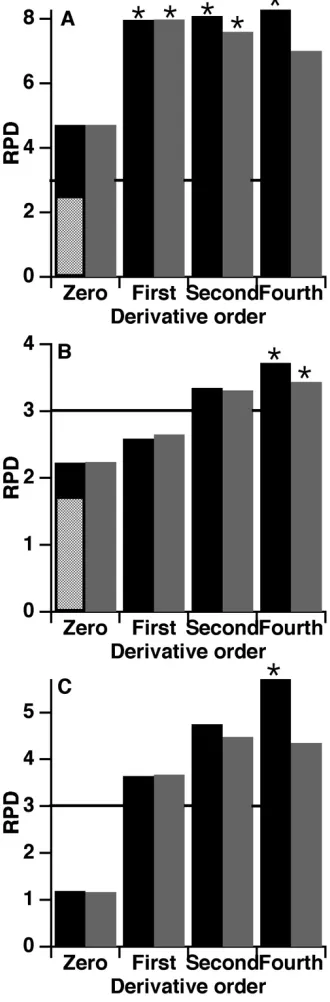
Figure 3.5 Summary of PLSR Results. This displays the highest RPD of the PLSR models of each preprocessing group. The threshold for an acceptable model (RPD = 3) is marked with a black line. Models not statistically different from the highest RPD model are marked with a black asterisk. Solid black bars represent GDs, dark grey represents SG derivatives, and light grey represents no preprocessing. For all 3 fabrics, GD4 achieves the highest RPD. The three panels correspond to: (a) Polyester Fabric, (b) Acrylic Fabric, and (c) Cotton Fabric ... 45
Figure 3.6 GD4 convolution function plotted with mean spectra of blood on polyester. The convolution function corresponds to the GD4 calibration using two gaps each of 6 and 48, one of the optimal combinations for calibration on polyester. The function comprises three triplets, sampling the curvature of the curvature of the spectra, also known as the fourth derivative. Note how the center and wing triplets are aligned with features of opposite curvature, the sweet spot for these matched filters. The center triplet also shows spacing to match two dips in the spectra on either side of the center peak. The relationship between these three points is closely related to the amount of blood solids present, again pointing to the optimization of gaps as a way of approximating a matched filter ... 55
clarity. The grey spectra show derivatives corresponding to RPD peaks: gaps = 2 and 7, 11, 16, 20, 25. The black spectra show derivatives corresponding to RPD valleys: gaps = 2 and 9, 13, 18, 23, 27. The grey traces appear to have higher noise levels, yet consistently perform much better than the gaps corresponding to the RPD valleys ... 64
Figure 3.8 Second latent variable for on- and off-feature models of blood on cotton fabric. The blue traces correspond to gap combinations just inside the outer ring visible in Fig. 3.4, and the red traces correspond to gap combinations just outside the outer ring. The black traces correspond to models corresponding to the gap combinations along the outer ring ... 67
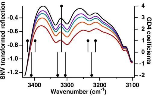
Figure 3.9 Difference spectrum of blood on cotton fabric in the Amide I/II region of the infrared spectrum. The GD coefficients (black lines, right axis) are for a GD4 function with g = 30 ... 69
Figure 3.10 Calibration metrics for models with gap combinations along the diagonal of Fig. 3.4c. The RPD is shown in black and reported on the right axis. The left axis shows the distance between LV1 and the blood component spectrum shown in Fig. 3.3c (blue) and the distance between LV2 and the difference between spectra collected on day 4 and day 1 (red). A distance of 1 indicates little overlap, while a distance of 0 indicates similarity ... 70
Figure 4.1 Spectral modification and differentiation. (a) The original spectrum of 25x dilute blood on cotton fabric. (b) The left side of the spectrum shown in (a) now padded to 3364 points (black). The associated weighting vector is also shown (grey, dashed). (c) The fourth-order RGD taken of the product of the padded spectrum and weighting vector shown in (b) ... 84
Figure 4.2 Difference between original spectrum and vector integrated from fourth-order RGD ... 90
the difference spectra in Fig. 4.3a, this time taken with different combinations of gap sizes. The combinations of gap sizes for the black traces are: 20,20,36,36; 24,24,34,34. The combinations of gap sizes for the red traces are: 20,20,40,40; 24,24,38,38; 30,30,34,34. The combinations of gap sizes for the blue traces are: 20,20,34,34; 24,24,32,32. The inset is an expansion of the Amide I and II region. The black traces correspond to gap sizes that have better calibration performance than the blue and red traces. The slightly different gap sizes cause noticeable changes in the difference spectra upon integration ... 101
Figure 4.5 Regression vectors (RV) for the PLSR calibrations. (a) The RV based on SNV-transformed data (black) and the integrated RV based on RGD transformed data normalized to unit variance (grey), both normalized to unit length. (b) The RV based on RGD transformed data normalized to unit variance in fourth-order space. The derivative RV appears much more convoluted than the zero-order analogue shown in the top panel. Generally, the integrated RV is less sensitive to changes in the NIR region (beyond 5000 cm-1) and features the amide bands more prominently ... 103
Figure 4.6 Integrated regression vectors (RVs) based on data in Fig. 4.3. The integrated RVs are normalized to unit length. The black traces corresponding to enhanced model performance show generally lower amplitude, and greater emphasis on the values near 1600 cm-1 relative to the amide bands than seen in the other RVs. The inset displays the second factor from the same models. The first weighting for each is similar, but this vector shows important differences. The black traces have a feature at 1600 cm-1, the area of the RV that is different, and the second factor is weighted more heavily in the definition of the RV. These factors demonstrate that small differences in gap size can cause larger differences in calibration that can best be explored by integrating the model vectors ... 105
Figure 5.1 The average SNV transformed reflection of blood on acrylic at 3300 cm-1 (corresponding to Amide A) shown as a function of inverse dilution factor (error bars are sample standard deviation)115
Figure 5.3 Relationship between coverage of blood solids and dilution factor. Each marker is the average coverage (mg/cm2) of blood added to 5 replicate sample squares of each fabric, offset by the apparent average value of the blank samples. The error bars are ± one standard deviation of the replicates ... 120
Figure 5.4 BET Isotherm Experiments. The results of the 5-point BET isotherm experiments are shown for each fabric. The legend records the sample mass, the line of best fit, and the specific surface area reported. All BET isotherm experiments were run on a Micromeritics ASAP 2020 in physisorption mode. ... 121
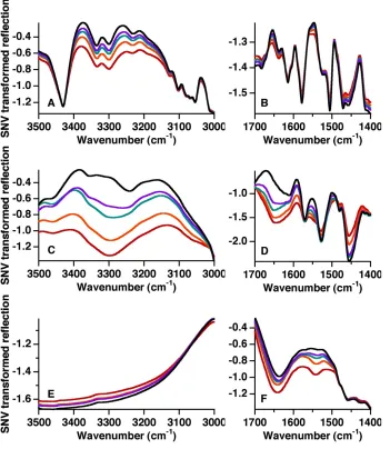
Figure 5.5 (a) Spectra of blood on acrylic and (b) calibration results. The spectra in (a) are acrylic fabric dip-coated from water (black), or blood diluted by a factor of 25 (red), 50 (orange), 100 (green), or 200 (blue). The inset is the mean derivative spectrum of the 25x dilute coated samples (red) and uncoated fabric (black) under the optimum conditions (LWMIR region) ... 128
Figure 5.6 (a) Spectra of blood on cotton and (b) calibration results. The spectra in (a) are cotton fabric dip-coated from water (black), or blood diluted by a factor of 25 (red), 50 (orange), 100 (green), or 200 (blue). The inset is the mean derivative spectrum of the 25x dilute coated samples (red) and uncoated fabric (black) under the optimum conditions (LWMIR region) ... 129
Figure 5.7 (a) Spectra of blood on polyester and (b) calibration results. The spectra in (a) are polyester fabric dip-coated from water (black), or blood diluted by a factor of 25 (red), 50 (orange), 100 (green), or 200 (blue). The inset is the mean derivative spectrum of the 25x dilute coated samples (red) and uncoated fabric (black) under the optimum conditions (SWMIR region) ... 130
Figure 5.8 Spectra of blood on nylon fabric. The SNV transformed spectra nylon fabric dip-coated from water (black), or blood diluted by a factor of 25 (red), 50 (orange), 100 (green), or 200 (blue). ... 131
increases with dilution factor. Spot sizes corresponding to these samples are recorded in Table 5.3 ... 139
Figure 6.1 (a) Visible image of the experiment set-up, viewed from the top as the infrared camera views it. The boxes show the regions of the image from which the bare electrode, painted electrode, and solution data were retrieved. (b) Infrared image of the experiment set-up ... 152
Figure 6.2 Cyclic voltammogram of 0.1 M K
3Fe(CN)6 in 1.0 M KNO3 run at scan rates of 100 mV/s, 500 mV/s, 750 mV/s, and 1000 mV/s. Scan direction is noted with an arrow. The CVs were collected with the set-up shown in Fig. 6.1 and described in the text. ... 154
Figure 6.3 Plot of emittance difference between the mean painted and bare metal electrode areas over the length of data collection (areas shown in Fig. 6.1). The overall upward slope shows the increase of electrode temperature with respect to the surrounding environment while the repeating higher frequency peaks correspond to cycles of voltammetry. ... 156
Figure 6.4 Plot of emittance difference between the mean painted electrode and mean solution over the length of data collection (areas shown in Fig. 6.1). The recurring peaks correspond to cycles of voltammetry. ... 157
Figure 6.5 Overlay plot of the average of voltammetry and thermometry results. Scan direction is noted with an arrow. Thermometry values are given by the difference between the painted electrode and the solution. ... 159
CHAPTER 1
INTRODUCTION
1.1. INFRARED SPECTROSCOPY AND FORENSIC SCIENCE
Crime scenes are often disordered environments, making it difficult to
identify samples that may be of forensic importance. Because biological evidence
such as semen, sweat, and blood may be found on any number of surfaces at a
variety of concentrations, it is important for investigators to have effective tools to
determine which samples might warrant further testing. These tools must be
selective enough to not waste resources on superfluous samples, sensitive
enough to detect small or dilute stains, and harmless enough that neither the
evidence nor the investigators will be adversely affected by their use.1
One of the most commonly used presumptive tests for the visualization of
blood is luminol, which undergoes a chemiluminsecent reaction with the heme
groups of blood.2 This chemiluminescence is visible in the dark.3 While luminol is
highly sensitive, it has a few drawbacks. Luminol is limited to use in a dark
environment,4 gives false positives for a variety of interferents,5 and has been
shown to reduce the recoverable quantity of DNA over time.6
Alternative light sources (ALS) are a potential alternative to detection by
currently available induce fluorescence of biological molecules or increase the
contrast between the biological evidence and its background, typically operating
in the ultraviolet and visible wavelength regions.1
Infrared (IR) spectroscopy has been suggested as another ALS system.
Infrared imaging and spectroscopy have been demonstrated for the analysis of
fabrics and bloodstains.7-10 Recently, a digital camera was sensitized to the
near-IR region to allow blood detection.11 The Myrick lab has recently reported a
thermal IR (8 – 14 µm) imaging system using reflectance imaging as a stand-off
technique to visualize blood on a fabric.12-14 This imaging system was based on
diffuse reflection (DR) IR spectroscopy, which has also been used to examine
fabric composition, dye state, and treatments.15-22 Near-IR reflectance
spectroscopy has been used to investigate blood stains. 23-24
In the forensic community, a common figure of merit for comparing
detection methods is the detection limit (DL), often reported in units of dilution
factor. The work presented in this dissertation seeks to establish a DL for blood
on fabric using IR DR spectroscopy. This analysis will allow comparison of
spectroscopic DLs to DLs using the more common luminol test. Further,
investigation of how DLs are influenced by both fabric substrates and spectral
windows can inform further instrument development, and the use of a
conventional benchtop FT-IR spectrometer will enable fundamental
1.2. DIFFUSE REFLECTION INFRARED SPECTROSCOPY
Infrared spectroscopy is a molecular spectroscopy technique used to
investigate the vibrational modes of an analyte. In an IR spectrum, fundamental
vibrations generally appear in the range of 400 – 4000 cm-1, which is the mid-IR
region.25 At the higher frequencies of the near-IR, weaker combination and
overtone absorbance bands appear. These are generally an order of magnitude
or more weaker than the fundamental bands.26 Our investigation of blood on
fabric leads us to look for absorbance bands related to proteins. These bands are
the Amide I (1650 cm-1), Amide II (1550 cm-1), Amide A (3300 cm-1), and Amide
B (3100 cm-1).27-29 Other bands less specific to proteins are also present in the
mid-IR related to peptide group vibrations and C-H deformation bands. The
Amide I band is characteristic of the hydrogen-bonded carbonyl stretch of the
peptide backbone. Amide II is related to both C-N stretching and N-H bending.
The broad Amide A feature corresponds to the N-H stretch of a secondary
amide, while the much weaker Amide B is the second overtone of the Amide II
bands strengthened by Fermi resonance with Amide A.27-29 These distinctive
features can be expected to form the basis of calibration for the presence of
blood on fabrics.
Transmission measurements are the most common application of IR
spectroscopy. However, transmission measurements are not feasible when the
spectroscopy measures the reflection from a sample collected at an angle not
equal to the angle of incident radiation, meaning it excludes the signal of
specular reflection. Fresnel diffuse reflection (FDR) and Kubelka-Munk, or
volume, reflection comprise the signal of DR.30-31 The volume reflection comes
from light that has undergone multiple reflection and refraction events before
being scattered out of the sample to the detector. Because of this, it carries
chemical information about the particles in the sample, enabling quantitative
analysis. When the sample is highly absorbing, any light that would carry this
signature is totally attenuated before it can be scattered out of the sample. When
that happens, FDR (the reflection off an irregular surface) contributes more
significantly to the signal.32 In our samples, this typically appears as an increase
in reflection in areas of high fabric absorbance as the surface coating increases.
This signal is not selective for the analyte concentration, so one would expect to
see that calibrations are best in regions of the spectrum where FDR contributes
minimally to the spectrum.
1.3. MULTIVARIATE CALIBRATION
Some features of IR DR spectra can cause difficulties in forming
calibrations. Because FDR is more closely related to the real portion of the
refractive index (rather than the imaginary portion related to absorbance),
anomalous dispersion can occur in the vicinity of strong absorbance features that
typically manifests as asymmetric peaks.30,32 An even more dominant feature of
DR spectra is the variability that arises primarily from scattering in the sample.
can impede further calibration. To prevent this from negatively influencing
calibration performance, spectral preprocessing is key.
One method often employed to eliminate baseline effects related to
scattering and other phenomena is derivative processing. Derivatives are well
known to improve calibration performance by eliminating baseline features and
increasing resolution of narrow or overlapping peaks.33-37 By coupling derivative
pretreatment with a correction for multiplicative effects such as the standard
normal variate transformation,38 most variable pathlength effects can be
removed.
After the spectra have been properly processed to minimize extraneous
variation, multivariate calibration techniques can be employed. These techniques
estimate the concentration of the analyte based on the relationship between
variables in the data block. Principal components analysis (PCA)39 and partial
least squares regression (PLSR) are two common multivariate calibration
techniques.40-41 Both approaches develop a regression vector (RV) that can be
used to predict analyte concentration in an unknown sample after calibration with
a known data set. This regression vector is a linear combination of the underlying
vectors, either principal components (PCs) or latent variables (LVs). In PCA, the
PCs maximize the explained variance in the spectral data set. In PLSR, the LVs
maximize the explained covariance of the spectral data set and the concentration
The performance of calibration models can be assessed by a few different
parameters. The four that will be used here are the root-mean-square error of
calibration (RMSEC), root-mean-square error of prediction (RMSEP), the ratio of
the standard deviation of the reference values to the RMSEP of the model
(RPD),42 and the DL.43-44 The RMSEC is given by:
Eq. 1.1. !!!!(!!!!!)! !
where n is the number of calibration samples, ! is the calibration prediction, and
y are the calibration reference values.45 To calculate the RMSEP, the validation
prediction and reference values are substituted in Eq. 1.1. The equations of the
RPD and the DL will be presented in Ch. 3 and Ch. 4, respectively.
1.4. DISSERTATION OUTLINE
Chapters 2-3 of this dissertation explore the implementation and
optimization of fourth-order gap derivatives (GDs) as an alternative to the more
common Savitzky-Golay (SG) smoothing derivatives. GDs approximate the
analytical derivative by calculating finite differences of spectra without curve
fitting. GDs offer an advantage of tunability for spectral data as the distance (gap)
over which this finite difference is calculated can be varied. Gap selection is a
compromise between signal attenuation, noise amplification, and spectral
resolution. A method and discussion of the importance of fourth derivative gap
selections are presented as well as a comparison to SG preprocessing and
lower-order GDs in the context of multivariate calibration. In most cases, we
better than SG derivatives, and that optimized fourth-order GDs behaved
similarly to matched filters.
Chapter 4 describes a modification to the GD algorithm to allow the
higher-order GDs and the RVs and LVs associated with PLSR models to be
integrated exactly. This exact integration allows better interpretation of how gap
selection influences calibration performance, and a demonstration of this
application is included.
Following the discussion of GD preprocessing, fourth-order GDs are used
in conjunction with PLSR to calibrate for blood on fabrics. The DLs are estimated
for IR DR spectroscopy using PLSR. While DLs often appear in terms of dilution
factor in the forensic community, mass percentage, coverage (mass per unit
area), or film thickness are often more relevant when comparing experimental
methods. These alternate DL units are related to one another and presented
here. The DLs for blood using IR spectroscopy are also compared to those
reported using luminol or an alternative IR imaging system
Chapter 6 deviates a bit from the theme by presenting a method to
investigate the heating at an electrode surface using an IR camera. This method
involves looking at the back surface of a platinum working electrode to examine
the heating and cooling cycles of the electrode in relation to the potential cycles
during a cyclic voltammetry experiment. Examination of this type offers insight to
extending the concept of GDs as matched filters to the development of matched
filters for spectral processing prior to multivariate calibration is presented.
Following that, the possibility of modifying PLSR calibrations to improve DLs by
minimizing variance of the predictions of blank samples is discussed. Initial
results show the possibility of DLs improved by a factor of 2 while using fewer
REFERENCES
(1) W. C. Lee, B. E. Khoo. “Forensic Light Sources for Detection of Biological Evidences in Crime Scene Investigation: A Review”. Malaysian Journal of Forensic Sciences. 2010, 1: 17-27.
(2) J. L. Webb, J. I. Creamer, T. I. Quickenden. “A comparison of the presumptive luminol test for blood with four non-chemiluminescent forensic techniques”. Luminescence. 2006. 21(4): 214-220.
(3) T. I. Quickenden, C. P. Ennis, J. I. Creamer. “The forensic use of luminol chemiluminescence to detect traces of blood inside motor vehicles”. Luminescence. 2004, 19: 271-277.
(4) K. Virkler, I. K. Lednev. "Analysis of body fluids for forensic purposes:
From laboratory testing to non-destructive rapid confirmatory identification at a crime scene". Forensic Sci. Int. 2009, 188(1): 1-17.
(5) T. I. Quickenden, J. I. Creamer. "A study of common interferences with the forensic luminol test for blood". Luminescence 2001, 16(4): 295-298.
(6) J. P. de Almeida, N. Glesse, C. Bonorino. "Effect of presumptive tests reagents on human blood confirmatory tests and DNA analysis using real time polymerase chain reaction". Forensic Sci. Int. 2011, 206(1): 58-61.
(7) G. van Dalen. "Protein on Cloths: Evaluation of Analytical Techniques". Appl. Spectrosc. 2000, 54(9): 1350-1356.
(8) A. Farrar, G. Porter, A. Renshaw. "Detection of Latent Bloodstains Beneath Painted Surfaces Using Reflected Infrared Photography". J. Forensic Sci. 2012, 57(5): 1190-1198.
(9) M. A. Raymond, R. L. Hall. "An Interesting Application of Infrared
Reflection Photography to Blood Splash Pattern Interpretation". Forensic Sci. Int. 1986, 31(3): 189-194.
(12) H. Brooke, M. R. Baranowski, J. N. McCutcheon, S. L. Morgan, M. L. Myrick. "Multimode Imaging in the Thermal Infrared for Chemical Contrast Enhancement. Part 1: Methodology". Anal. Chem. 2010, 82(20): 8412-8420.
(13) H. Brooke, M. R. Baranowski, J. N. McCutcheon, S. L. Morgan, M. L. Myrick. "Multimode Imaging in the Thermal Infrared for Chemical Contrast Enhancement. Part 2: Simulation Driven Design". Anal. Chem. 2010, 82(20): 8421-8426.
(14) H. Brooke, M. R. Baranowski, J. N. McCutcheon, S. L. Morgan, M. L. Myrick. "Multimode Imaging in the Thermal Infrared for Chemical Contrast Enhancement. Part 3: Visualizing Blood on Fabrics". Anal. Chem. 2010, 82(20): 8427-8431.
(15) M. R. Pearl, H. Brooke, J. N. McCutcheon, S. L. Morgan, M. L. Myrick. "Coating Effects on Mid-Infrared Reflection Spectra of Fabrics". Appl. Spectrosc. 2011, 65(8): 876-884.
(16) N. M. Morris. "A Comparison of Sampling Techniques for the
Characterization of Cotton Textiles by Infrared-Spectroscopy". Text. Chem. Color. 1991, 23(4): 19-22.
(17) S. Ghosh, M. D. Cannon, R. B. Roy. "Quantitative-Analysis of Durable Press Resin on Cotton Fabrics Using near-Infrared Reflectance
Spectroscopy". Text. Res. J. 1990, 60(3): 167-172.
(18) C. Gilbert, S. Kokot. "Discrimination of Cellulosic Fabrics by
Diffuse-Reflectance Infrared Fourier-Transform Spectroscopy and Chemometrics". Vib Spectrosc. 1995, 9(2): 161-167.
(19) C. Gilbert, S. Kokot, U. Meyer. "Application of Drift Spectroscopy and Chemometrics for the Comparison of Cotton Fabrics". Appl. Spectrosc. 1993, 47(6): 741-748.
(20) S. Kokot, K. Crawford, L. Rintoul, U. Meyer. "A DRIFTS study of reactive dye states on cotton fabric". Vib. Spectrosc. 1997, 15(1): 103-111.
(21) H. M. Heise, R. Kuckuk, A. Bereck, D. Riegel. "Mid-infrared diffuse reflectance spectroscopy of textiles containing finishing auxiliaries". Vib. Spectrosc. 2004, 35(1): 213-218.
(23) E. Botonjic-Sehic, C. W. Brown, M. Lamontagne. M. Tsaparikos. "Forensic Application of Near-Infrared Spectroscopy: Aging of Bloodstains".
Spectroscopy 2009, 24(2): 42-48.
(24) G. Edelman, V. Manti, S. M. van Ruth, T. van Leeuwen, M. Aalders. "Identification and age estimation of blood stains on colored backgrounds by near infrared spectroscopy". Forensic Sci. Int. 2012, 220(1): 239-244.
(25) B C. Smith. Fundamental of Fourier Transform Infrared Spectroscopy. New York: CRC Press, 1996.
(26) J. M. Olinger, P. R. Griffiths. “Theory of Diffuse Reflectance in the NIR Region”. In: D. A. Burns, E. W. Ciurczak, editors. Handbook of Near-Infrared Analysis. New York: Marcel Dekker, Inc., 1992
(27) J. T. Kuenstner, Norris, K. H., V. F. Kalasinsky. "Spectrophotometry of Human Hemoglobin in the Midinfrared Region". Biospectroscopy. 1997, 3: 225-232.
(28) K. T. Hecht, D. L. Wood. "The near Infra-Red Spectrum of the Petide Group". Proc. R. Soc. A. 1956, 235(1201): 174-188.
(29) A. J. Sadler, J. G. Horsch, E. Q. Lawson, D. Harmatz, D. T. Brandau, C. R. Middaugh. "Near-Infrared Photoacoustic-Spectroscopy of Proteins". Anal. Biochem. 1984, 138(1): 44-51.
(30) P. J. Brimmer, P. R. Griffiths, N. J. Harrick. “Angular-Dependence of Diffuse Reflectance Infrared-Spectra .1. Ft-Ir Spectrogoniophotometer”. Appl. Spectrosc. 1986, 40(2): 258-265.
(31) M. L. Myrick, M. N. Simcock, M. Baranowski, H. Brooke, S. L. Morgan, J. N. McCutcheon. “The Kubelka-Munk Diffuse Reflectance Formula
Revisited”. Appl. Spectrosc. Rev. 2011, 46(2): 140-165.
(32) M. L. Myrick, S. L. Morgan. “Infrared Specular Reflection Calculated for Polymer Films on Polymer Substrates: Models for the Spectra of Coated Plastics”. Spectroscopy. 2012, 40-56.
(33) W. L. Butler. "Fourth Derivative Spectra". Methods Enzymol. 1979. 56: 501-515.
(36) J. E. Cahill. "Derivative Spectroscopy - Understanding Its Application". Am. Lab. 1979. 11(11): 79-85.
(37) K. H. Norris, P. C. Williams. "Optimization of Mathematical Treatments of Raw Near-Infrared Signal in the Measurement of Protein in Hard Red Spring Wheat. 1. Influence of Particle-Size. Cereal Chem. 1984. 61(2): 158-165.
(38) R. J. Barnes, M. S. Dhanoa, S. J. Lister. "Standard Normal Variate Transformation and De-Trending of Near-Infrared Diffuse Reflectance Spectra". Appl. Spectrosc. 1989. 43(5): 772-777.
(39) M. Hubert. "Robust Calibration". In: P. J. Gemperline, editor. Practical Guide to Chemometrics. New York: Taylor & Francis, 2006. 2nd ed. Ch. 6, Pp. 167-215.
(40) M. Sjostrom, S. Wold, W. Lindberg, J. Persson, H. Martens. “A
Multivariate Calibration Problem in Analytical chemistry Solved by Partial Least-Squares Models in Latent Variables”. Anal. Chim. Acta. 1983, 150: 61-70.
(41) S. de Jong. “SIMPLS: an alternative approach to partial least squares regression”. Chemom. Intell. Lab. Syst. 1993, 18: 251-263.
(42) P. C. Williams. "Implementation of Near-Infrared Technology". In: P. C. Williams, K. H. Norris, editors. Near-Infrared Technology in the Agricultural and Food Industries. St. Paul, USA: American Association of Cereal
Chemists, 2001. 2nd ed. Ch. 8, Pp. 145-170.
(43) L. A. Currie. "Nomenclature in Evaluation of Analytical Methods Including Detection and Quantification Capabilities". Pure Appl. Chem. 1995, 67(10): 1699-1723.
(44) R. Boqué, F. X. Rius. "Multivariate dection limits estimators". Chemom. Intell. Lab. Syst. 1996, 32: 11-23.
CHAPTER 2
INFLUENCE OF GAP SELECTION ON THE PERFORMANCE OF GAP DERIVATIVES
2.1. INTRODUCTION
Derivatives are a commonly applied preprocessing tool for multivariate
calibration. Derivatives offer many benefits, including reducing the effect of
baseline slope or offset, resolving overlapping peaks, and enhancing narrow
features.1-4 Derivatives also have some drawbacks impeding their
implementation. Derivative spectra are more complicated than their zero-order
analogues, featuring n + 1 peaks for each peak in the original spectrum (where n
is the derivative order).1 These extra peaks appear as side lobes that interfere
with one another and with neighboring peaks, causing reduction of peak heights
or development of artificial peaks. Further, compromises must be struck when
optimizing parameters to balance resolution enhancement, signal distortion,
noise amplification, and signal attenuation in the derivative spectrum.5
Two of the most commonly applied derivatives are Savitzky-Golay (SG)
smoothing derivatives and segment-gap derivatives. This work will focus on the
use of segment-gap derivatives which approximate the analytical derivative (AD)
cases, the segment is equal to one and no averaging occurs, resulting in a
simple gap derivative (GD), sometimes referred to as a finite difference, Norris,
or Butler-Hopkins derivative.1-3,7-10 GD computation is often coupled with a
smoothing routine, though that is not always necessary or desirable. Higher order
derivatives are obtained by repeating the differentiation sequentially.
The greatest impetus for using SG derivatives rather than GDs is the
smoothing effect of fitting a polynomial to the data first. However, GDs coupled
with smoothing routines or using different gap sizes for iterative differentiation
have been shown to yield results comparable to or better than SG.8-10 Other work
has shown that each GD performed with gap g is similar to a g-point sliding
average smooth.4,11 Further, early workers suggested that in systems with lower
noise levels, smoothing would be less necessary and higher-order derivatives
with greater resolution enhancement would be favored for use.1-3,12-13 With the
advent and widespread use of interferometry in the infrared, spectra now have
noise levels consistently low enough to favor the use of higher-order derivatives
without the need for separate smoothing routines.
The usefulness of GDs largely depends on the selection of an appropriate
gap size for the calculation. Previous literature has explored the influence of gap
size on spectral shape and intensity, generally focusing on maximizing peak
resolution while minimizing noise influences and signal distortion. The general
observations included decreasing signal-to-noise ratio (SNR) with increasing
derivative order, increasing SNR with increasing gap size, and advantages
thus far been a gap size approximately equal to the full-width at half-maximum
(FWHM) of the peak of interest.1-4,8-10,12,14 This work will present the calculation of
GDs and demonstrate the influence of gap selection on the resulting derivative
signal and noise.
2.2. GAP DERIVATIVE CALCULATION
The equation for computing the GD comes in a variety of forms in the
literature, differing primarily on two points: how the gap (distance between points
used in the calculation) is defined and whether to divide the difference in spectral
intensity by the gap.2,7,14 The fundamental concept of the derivative is the slope
of the zero-order spectrum, the change in y divided by the change in x.4 This
basic definition leads to the equation of a first-order derivative:
Eq. 2.1 !! ! = !!!!/! !!(!!!/!) !
where g is the defined gap size.4 As discussed earlier, this operation can be
repeated on the data n times to yield the nth-order derivative. This iteration will
yield a convolution function with coefficients given by the nth row of Pascal’s
triangle.1 The second-order derivative, when the same gap is chosen for each
derivative step, is given by:
Eq. 2.2 !!! ! = !!!! !!!! !!(!!!) !!
For each derivative calculated, a new gap can be selected. By using n
different gaps (a unique gap for each iteration of the derivative calculation), a
used in the calculation does not influence the final derivative. The equation for a
fourth-order derivative in the same form as the preceding equation is:
Eq. 2.3 !!!!! ! = !!!!! !!!!!! !!!! !!!!!! !!!!!! !!
2.3. INFLUENCE OF GAP SIZE ON DERIVATIVE SHAPE FOR A LORENTZIAN BANDSHAPE
A Lorentzian lineshape is described by Eq. 2.4,
Eq. 2.4 != !!!!!!!!
! !!!
where !! is the center of the band and Γ is the FWHM of the lineshape. For our
discussion below, we generalize the function by introducing the unitless variables
!= ! !!"# and != !−!! Γ, reducing Eq. 2.4 to the form:
Eq. 2.5 ! =!!!!!!
(see Fig. 2.1a). Expressions for the ADs and GDs of ! for orders 1, 2, and 4 are
provided in Table 2.1, where the unitless gap ! = !/Γ is introduced for the GDs
to relate the implemented gap size in terms of a fraction of the FWHM of the
Lorentzian. From Table 2.1, it is evident that the GD approaches the AD for each
order as ! approaches zero.
Figure 2.1b-d illustrate the influence of gap size and derivative order on
the magnitude of the resulting derivative function for the curve in Fig. 2.1a. The
first-, second-, and fourth-order GDs are shown with ! = 0.1, 0.5, 1, and 2, along
with the AD. As the derivative order increases, the maxima and minima of GDs
deviate more from the corresponding ADs proportionally to the FWHMn (Thus,
Table 2.1: Derivatives of ! with respect to !, simplified by the introduction of variable != 4!!+1.
n Derivative Analytical Gap Derivative
0 !
!
1 !!!
!!
!!!
!!!!!!!!!!!!!!!!!!!!
2 !!!"!!!!! !!
!!!"!!!!!!!!!
!!!!!!!!!!!!!!!!!!!!!!!!!
4 !"#!!"!!!!"!!!!! !!
!"# !"!!!!"#!!!!!!"!!!!"!!!!"!!!!
!"!!!!"!!!! !!!!!!!!! ! !!!!!!!!! !"!!!!"!!!!
point that GD1 determined with ! = 2 no longer appears as a derivative; rather,
the trace resembles a positive image of the band shifted by -! connected to a
negative image of the band shifted by +!. Both of these images of the band have
an intensity approximately one-half that of the original band. As ! is increased
beyond 1, the GD no longer offers a good approximation of the AD. Because of
this, narrow gaps are preferred for the purpose of simulating a true AD for visual
inspection.2
When different gap sizes are used for each iteration of the derivative
calculation, the resulting GD deviates from both the AD and the above noted
trends in the relationship between gap size, derivative order, and the GD shape
(black traces in Fig. 2.1c-d). For example, the GD2 calculated with !! = 0.1 and
!! = 0.5 has a maximum intensity intermediate between that obtained with either
gap size !! or gap size !!, alone (Fig. 2.1c). Similarly, GD4 calculated with four
different gaps (!! = 0.1, !! = 0.5, !! = 1, !! = 2) does not simply resemble the
derivative calculated with any single gap size (Fig. 2.1d); the center peak of that
GD4 spectrum inverts relative to the center peak of the other GD4 spectra.
Though this deviation from the expected derivative shape may complicate peak
identification by visual inspection, it will be consistent among similar peaks and
should not necessarily be expected to impede multivariate calibration.4
2.4. INFLUENCE OF GAP SIZE ON SNR FOR A LORENTZIAN BANDSHAPE
with noise added to give a SNR = 10. The GD4 with ! = 0.1, in which the
Lorentzian derivative feature is completely obscured by noise, is shown in Fig.
2.2b. The GD4 calculated with ! = 1 is shown in Fig. 2.2c. Here, the central peak
has become visible above the noise once again, despite the much lower signal
value of the GD. In this case, the wider gap is preferable to the narrow gap
because the wide gap offers an advantage of effectively smoothing the noise as
the derivative is calculated, preventing the noise from masking the signal.
The maximum signal magnitude of a GD is related to the original signal
magnitude as shown in Fig. 2.3, drawn to log scale (solid traces in left column).
Table 2.2 gives equations for the maximum signal magnitude of GD1, GD2, and
GD4 as a function of the gap size !. The magnitudes of all these derivatives fall
as !!! for large ! where n is the derivative order. For GD1, the position of the
maximum signal amplitude is not at the center of the Lorentzian band, resulting in
a more complicated formula. For even-order derivatives, the maximum signal
magnitude is located at != 0, the center of the Lorentzian band. All the signal
magnitudes are greatest with ! ≥ 0, with magnitudes of ! !! , 8, and 384 for GD1,
GD2, and GD4, respectively. All these signal magnitudes fall as a function of
increasing ! with a somewhat Lorentzian form. For GD2, this form is explicitly
Lorentzian with Γ!"# =1. The GD4 signal magnitude falls as the product of two
Lorentzians, one with Γ!"#$ =1 and the other with Γ!"#$ = 0.5.
Assuming the noise is equal at every wavelength channel in the original
Table 2.2: Maximum values of GDs.
Order Gap Derivative Maximum
1 3 −3+3!!+6 !!+!!+1
−!! −3+3!!+6 !!+!!+1 + 2!!+ !!+!! +1+1 !
2 −8
(4!!+1)
4 384
according to Eq. 2.6:
Eq. 2.6 σ!"! = σ! !! ! !!! !!! !!
where ci is the ith binomial coefficient in the nth row of Pascal’s triangle and σ! is
the standard deviation of the noise in a channel of the original spectrum. This
equation is obtained by propagation of errors from a definition of the GD with a
single gap in terms of the original spectral channels (Eq. 2.2). The noise in the
GDs (Fig. 2.3, dashed traces in left column) falls as a function of ! more quickly
than the GD signal for small and intermediate !. This suggests that the SNR of
the derivative spectrum will improve with increasing gap size for small and
intermediate ! and plateau for larger values of !. This is found to be the case, as
shown in the right column of Fig. 2.3. For each derivative order, the SNR of the
derivative spectrum increases rapidly as ! approaches about 0.8. The SNR then
tends toward a plateau as ! ~ 2. However, regardless of the value of !, the
derivative spectra using a single value of ! have lower SNR values than the
original spectrum from which they were created. For instance, for ! = 1, GD1,
GD2, and GD4 have relative SNRs (SNRn/SNR0) of 0.57, 0.65, and 0.54,
respectively, where SNR0 is the signal-to-noise ratio of the original spectrum and
SNRn is the signal-to-noise ratio of the GDn spectrum. SNRn for all n is
degraded compared to the original spectrum, with the least degradation found in
the second-order derivative. The lack of a clear trend in these values is a result
of comparing even and odd orders of differentiation.
calculated with a different gap size ! for each step of differentiation. The signal is
not degraded further if the additional gap sizes incorporated do not diminish the
signal significantly. The SNR of nth-order GDs calculated with multiple gaps
(SNRnmg) with this constraint is approximated by:
Eq. 2.7 SNR!!" ≈SNR! !!!!!! !!! !!
where again the coefficients squared in the summation are from row n of
Pascal’s triangle. Since the sum of the elements of row n of Pascal’s triangle
always equals 2n, and since no values found in the triangle are less than unity,
the SNRn (n>1) of a higher-order GD when multiple values of ! are used will
always exceed the SNR of the same GD when a single ! is used. Because only
one gap is possible in GD1, it is not improved by using multiple gaps in this way,
but could be improved by a gap-segment approach with a segment greater than
one that is not discussed here.6-7
Relative SNRnmg for GDs is shown in dashed traces in the right column of
Fig. 2.3. The relative SNR2mg (with !! and !! both approximately 1) of GD2 is
now improved by a factor of 6 4, to 0.80, and continues to increase with !
although never exceeding unity. For GD4, the improvement is 70 16, resulting
in a relative SNR4mg of 1.13 with all ! values close to 1. In this case, SNR4mg
exceeds that of SNR0, and continues to increase with ! up to a maximum of
2.5. CONCLUSIONS
The selection of gap sizes used in the calculation of GDs at any order is a
compromise between noise and signal. While small gap sizes might be preferred
to approximate an analytical derivative, they have the disadvantage of
decreasing the SNR of the derivative spectrum. Large gap sizes effectively
smooth high-frequency noise in the derivative spectrum, but also tend to reduce
the amplitude of narrow spectral features. The shape of spectral features that
should be highlighted or resolved from spectral interferences will largely influence
the optimal gap combination for GD spectral processing. The next chapter will
demonstrate how this interplay influences gap selection for the calibration of
REFERENCES
(1) W. L. Butler. "Fourth Derivative Spectra". Methods Enzymol. 1979. 56: 501-515.
(2) W. L. Butler, D. W. Hopkins. "Analysis of Fourth Derivative Spectra". Photochem. Photobiol. 1970. 12(6): 451-456.
(3) W. L. Butler, D. W. Hopkins. "Higher Derivative Analysis of Complex Absorption Spectra". Photochem. Photobiol. 1970. 12(6): 439-450.
(4) J. E. Cahill. "Derivative Spectroscopy - Understanding Its Application". Am. Lab. 1979. 11(11): 79-85.
(5) R. I. Shrager. "Some Pitfalls in the Use of Derivative Spectra". Photochem. Photobiol. 1983. 38(5): 615-617.
(6) D. W. Hopkins. "What is a Norris derivative?". NIR news. 2001. 12(3): 3-5.
(7) K. H. Norris, P. C. Williams. "Optimization of Mathematical Treatments of Raw Near-Infrared Signal in the Measurement of Protein in Hard Red Spring Wheat. 1. Influence of Particle-Size. Cereal Chem. 1984. 61(2): 158-165.
(8) W. F. Maddams, W. L. Mead. "The Measurement of Derivative
IR-Spectra. 1. Background Studies". Spectrochim. Acta, Part A. 1982. 38(4): 437-444.
(9) S. Hawkes, W. F. Maddams, W. L. Mead, M. J. Southon. "The
Measurement of Derivative IR-Spectra. 2. Experimental Measurements". Spectrochim. Acta, Part A. 1982. 38(4): 445-457.
(10) W. F. Maddams, M. J. Southon. "The Measurement of Derivative IR-Spectra. 3. The Effect of Bandwidth and Band Shape on Resolution Enhancement by Derivative Spectroscopy". Spectrochim. Acta, Part A. 1982. 38(4): 459-466.
(13) W. F. Maddams. "The Scope and Limitations of Curve Fitting". Appl. Spectrosc. 1980. 34(3): 245-267.
CHAPTER 3
OPTIMIZED GAP DERIVATIVES AS MATCHED FILTERS
3.1. INTRODUCTION
The theoretical work described in the previous chapter demonstrated how
the selection of gap sizes in gap derivative (GD) preprocessing routines could
greatly influence the resulting derivative quality. Of particular interest is the
demonstration of how the noise in the derivative can be suppressed relative to
the noise in the original signal by incorporating multiple gap sizes in the
calculation of higher-order derivatives. As mentioned in Chapter 2,
Savitzky-Golay (SG) derivatives are typically favored over GDs to approximate the
analytical derivative (AD) because of the smoothing inherent in their calculation:
SG derivatives are determined by taking the AD of a polynomial fit to a region
(the window) of the spectrum. This smoothing effect suggests that calibrations
performed with SG derivatives should always perform comparably to or better
than GDs.1-2 However, if appropriate gap sizes are used for the GD calculation,
this may no longer be expected to hold true.
This chapter compares the performance of first-, second-, and fourth-order
derivatives calculated by the SG and GD methods to enhance multivariate
greatest influence on the calibration. The gap size combinations were optimized
for GDs by partial least-squares regression (PLSR) for the purposes of relative
quantification rather than the more traditional application to peak identification
and resolution. Optimum GD functions, particularly fourth-order GD functions, are
acting in part as matched filters for analyte spectral features.
3.2. METHOD
3.2.1. Sample Preparation Twenty-five sample squares (2” X 2”) each of
triple-dyed, unfinished brown polyester, purple acrylic, and red cotton fabrics
were cut from large swatches. These samples were sonicated for 60 min in
deionized (DI) water and suspended to dry for about 24 h. Five squares of each
fabric were dip-coated from each of the following solutions: (1) DI water, (2) 25x
dilute rat blood in DI water, (3) 50x dilute rat blood in DI water, (4) 100x dilute rat
blood in DI water, (5) 200x dilute rat blood in DI water. The treated fabrics were
again suspended to dry before spectroscopic measurements. Five replicate
sample sets were created for each fabric by grouping one sample square of each
of the 5 solutions into a set.
3.2.2. Spectral Collection Infrared diffuse reflection spectra were collected on a
Thermo-Nicolet Nexus 470 FT-IR spectrometer (Thermo Electron, Madison, WI)
with a U-Cricket diffuse reflectance accessory (Harrick Scientific Products,
Pleasantville, NY). A two-inch diameter gold diffuse reflection standard was used
as a reference (Optronics Laboratories, Inc.). Twenty replicate spectra were
collected from each of the 75 fabric squares by translating the fabric square over
that source of spectral variability. All the spectra of each sample set were
collected in one day, with the spectra of replicate sample sets collected over five
consecutive days. Parameters for spectral acquisition were: 600-7000 cm-1
spectral range (3320 spectral points), 64 scans, 4 cm-1 resolution, laser
modulation frequency of 10 KHz, Happ-Genzel apodization, and Mertz phase
correction. The spectrometer uses a liquid nitrogen cooled MCT detector and KBr
beamsplitter and is operated by OMNIC® software (Thermo, Madison, WI).
3.2.3. Outlier Detection Data were saved as text files in OMNIC® and
processed with MATLAB 7.13 (The MathWorks, Inc., Natick, MA). Prior to
calibration, spectra were tested for outliers. Spectra were normalized by the
standard normal variate transform3 (SNV) and decomposed by principal
component analysis. The spectra of each dilution were tested for outliers by
Hotelling’s T-squared test statistic.4 Outliers were removed from further analysis.
The sample sets were then tested against one another. Of the five sample sets,
no sets were detected as outliers. However, due to a change in the accessory,
the spectra of one sample set of each fabric appeared to be outliers upon visual
inspection of the data and so were removed from further analysis. The remaining
data were split into calibration and validation sets, with three sample sets
retained for calibration (~60 spectra at each dilution for each fabric) and one
sample set retained for validation (~20 spectra at each dilution) of the model.
samples that were retained for analysis. Figure 3.3a-c shows the difference
between the mean spectra of 25x dilute blood on fabric and neat fabric.
3.2.3. Data Preprocessing We combine derivative preprocessing with
SNV preprocessing. First-order derivative processing is often considered a
means of removing a baseline offset from spectral data. SNV also removes
baseline offset, as well as adjusts the span of the data and corrects multiplicative
effects. Because SNV offers the additional benefit of reducing multiplicative
effects, the two processing methods perform complementarily with one another.
When first derivative processing is applied to spectral data prior to SNV, the
effects of any baseline offsets are eliminated, and any curvature in the baseline
is also converted into a new baseline offset.5-6 Thus the combination of
differentiation in the nth degree followed by SNV is to remove a polynomial of
order n+1 from the original spectral data, as well as to change the weights
accorded to spectral features according to their relative shapes and to give a
common breadth to the resulting profiles prior to modeling. When working with IR
reflectance spectra, the data are often transformed to pseudo-absorbance data
by applying a log(1/R) treatment prior to further processing in hopes of linearizing
the relationship between spectra and concentration. We investigated whether this
pretreatment used in conjunction with SNV and derivative processing would
improve our results. While implementing this pretreatment did change the
emphasis on certain features shown in Fig. 3.4 (and described later), the log
transform did not improve calibration results as a whole because the combination
spectra. Accordingly, this transform was not implemented. For SG preprocessing,
zero-, first-, second-, and fourth-order derivatives (SG0, SG1, SG2, and SG4,
respectively) were taken of quadratic and quartic polynomials. The window frame
of the polynomial fit was varied from 5 to 101 (odd values).7 For GD
preprocessing, first-, second-, and fourth-order derivatives (GD1, GD2, and GD4,
respectively) were calculated. The gaps for all GD1 calculations were varied from
2 to 50 (even integers). GD2s were calculated by two first derivative iterations
with two distinct gaps (even integers from 2 to 50), or with one second derivative
iteration with one gap (integers from 2 to 50). GD4s were calculated by four first
derivative iterations four distinct gaps (even integers from 2 to 50), or two
second-derivative iterations with two gaps (integers from 2 to 50).
In calculating GDs, data points at either end of the spectrum are lost. The
number of points lost is equal to one-half the sum of the gaps used. To ensure
that the comparison of preprocessing methods was not influenced by these
missing points, each derivative spectrum was trimmed to the length of the
shortest derivative.
3.2.4. Calibration After derivative preprocessing, data were transformed by
SNV and mean-centered prior to PLSR performed using PLS toolbox 6.7.1
(Eigenvector Research Inc., Wenatchee, WA). All spectral points remaining after
derivative processing were used in every calibration (793 – 6808 cm-1). Previous
solids deposited, we calibrate the method to the inverse dilution factor of the
dipping solution, knowing this is directly proportional to the mass of blood solids
on the dried fabrics, although the proportionality constant is different for each
fabric depending largely on the exposed surface area of the fibers from which the
fabric is made. For a more consistent comparison, the same number of latent
variables (LVs) was retained in all models. Two LVs were retained for each
model, as two LVs was indicated as the most common optimum number of LVs
to be retained by the mean-square error of prediction (RMSEP) and the
root-mean-square error of cross validation (RMSECV) of the models.
The ratio of the standard deviation of the reference values to the RMSEP
of the model (known as the RPD)9 was calculated for each model as:
Eq. 3.1 RPD=σ!/RMSEP
The RPD provides a framework to interpret the RMSEP in terms of the model
performance in predicting unseen data by assessing model performance against
simply predicting the mean value of the validation set for each sample. A
threshold RPD of three has been previously suggested as a minimum for
adequate model performance and only models performing better than this
threshold were retained.9 Of the remaining models, the calibration model
selected was that with the lowest RMSEP.
The model with the overall lowest RMSEP for each fabric was then
compared to the model with the lowest RMSEP within each preprocessing group
of that fabric. The preprocessing group is the set of all models of a given
of these models were compared against the overall lowest RMSEP model to test
for significance at 95% confidence, according to the method published by
Fearn.10
3.3. COMPARISON OF DERIVATIVE PROCESSING METHODS IN INFRARED DIFFUSE REFLECTION SPECTROSCOPY
Derivative processing provides advantages – rejection of baseline offsets,
slopes and curvatures, in addition to changing the relative importance of spectral
bands – for pretreating diffuse reflection spectra prior to chemometric modeling.
The SG and GD approaches to differentiating spectra are computationally
distinct. The seemingly implicit noise suppression of SG derivatives make them
attractive, particularly for visual inspection. However, as shown in Chapter 2, the
reputation that GDs have for generating noisy derivatives is only deserved for
small gaps that attempt to preserve the appearance of a true AD. If we allow GDs
with larger gaps, noise is suppressed, and can even become lower than that of
the original spectrum, without introducing any specific smoothing functions. The
question remains whether the two approaches are comparable for modeling data
using chemometric methods. In this section, we apply both methods to the
measurement of the amount of blood solids on three different types of fabrics,
using a brute force approach to comparing and evaluating SG and multiple-gap
GD processing of spectroscopic data as an input for the calibration models.
The averaged spectra for the different fabrics shown in Fig. 3.1 and 3.2
solids are attributable to blood proteins, primarily the Amide I and II bands (near
1650 and 1540 cm-1, respectively), and the broader Amide A and B bands (near
3220-3300 and 3080 cm-1, respectively), as well as some of the weaker protein
bands. Both of these features are clearly visible in the spectrum of blood on
acrylic, and the Amide A band is particularly prominent (Fig. 3.2c-d, Fig. 3.3b). In
this case, Amide A appears with a FWHM of about 92 cm-1 (48 points). While the
Amide I/II peaks are also visible in the spectra, the matrix spectrum of acrylic
also exhibits many features similar in shape and intensity throughout the
mid-infrared region. The Amide I band has an apparent FWHM of about 34 cm-1 (18
points) and the Amide II band appears about half as wide, with FWHM of 17 cm-1
(9 points). Hemoglobin is the dominant protein in blood, and a spectrum of
hemoglobin can be found in a protein spectral database at University of Northern
Colorado.11 In the spectral database, the FWHM of hemoglobin’s Amide I band is
estimated at 34 cm-1, and the Amide II has a comparable width. In our spectra,
the Amide II appears narrower because of strong underlying absorption from the
fabric. As a result of the strong acrylic absorbance in this region, there is a
general increase in reflectance in the mid-infrared that may be attributed to the
presence of a coating on the fabric, though it might not be particularly useful in
developing calibrations.8 The Amide A absorbance is also prominent in the
spectrum of blood on polyester (Fig. 3.2a-b), though it is not as isolated as it
appears in the spectrum of acrylic. Instead of a single, broad band, Fig. 3.3a
shows a group of three overlapping peaks in the Amide A region. The central
points), much narrower than the Amide A band in acrylic. The FWHM of the
feature combining the three smaller bands is about 206 cm-1 (107 points). While
the Amide A is visible even when overlapped with polyester features, polyester
strongly absorbs in the same region as the Amide I/II absorbance, rendering the
Amide II band just visible upon close inspection and Amide I obscured. In
contrast, the strong hydroxyl absorbance of cotton entirely masks the Amide A
absorption (Fig. 3.2e-f). The strength of the absorbance in this region leads to an
increase in surface reflection at that wavelength region due to the presence of a
coating (Fig. 3.3c). The Amide II peak, though, falls in a region of relatively high
cotton reflectance and so is clearly visible in this case. The Amide I band,
however, is obscured as it is located along a steeply sloping region of the cotton
spectrum. Despite this overlap, both the Amide I and Amide II peaks appear
strongly in the difference spectrum, both with similar FWHM values of
approximately 40 cm-1 (20 points), values close to those reported for the
spectrum of hemoglobin.
Models were constructed using the procedure described above. The
calibration parameters resulting in the lowest RMSEP (highest RPD) of each
preprocessing method for blood-coated polyester, acrylic, and cotton fabrics are
reported in Tables 3.1 - 3.3, while Fig. 3.5 graphically represents the
performances of the best performing models for each derivative order by both SG