A Computational Method with MAPLE for a Piecewise Polynomial Approximation to the Trigonometric Functions

(1)

Article

A Computational Method with MAPLE for a

Piecewise Polynomial Approximation to the

Trigonometric Functions

Le Phuong Quan1*

1 _{Department of Mathematics, College of Natural Sciences, Cantho University, 3/2 Street, Cantho City,}

Vietnam; lpquan@ctu.edu.vn

* Correspondence: lpquan@ctu.edu.vn

Abstract: A complete MAPLE procedure is designed to implement effectively an algorithm for approximating the trigonometric functions. The algorithm gives a piecewise polynomial approximation on an arbitrary interval, presenting a special partition that we can get its parts, subintervals with ending points of finite rational numbers, together with corresponding approximate polynomials. The procedure takes a sequence of pairs of interval-polynomial as its output that we can easily explore in some useful ways. Examples on calculating approximate values of the sine function with arbitrary accuracy for both of rational and irrational arguments as well as drawing the graph of the piecewise approximate functions will be presented. Moreover, from the approximate integration of integrands of the formxmsinxon[a,b], another MAPLE procedure is proposed to find the desired polynomial estimates in norm for the bestL2-approximation of the sine function in the vector space P_`of polynomials of degree at most`, a subspace ofL2(a,b).

Keywords: approximation; approximate value; evaluation error, approximation error; piecewise approximate polynomial; rational approximation; Taylor’s Theorem

MSC:41A10, 42A10, 65D17, 65D18

1. Introduction

There would be the two aspects of implementation of an algorithm. One is the illustration for the validity of the algorithm, and another for the efficient exploration of its steps thanks to the choice of suitable tools.

Remez’s minimax algorithm is well established (see [4, Sec. 3.5]), but all the steps to proceed it contain the two main obstacles when being performed in practice:

• solving a nonlinear equation and a system of linear equations; • using the cosine function to compute the initial set of points.

As warned to experienced users, they should have close control of the evaluation error at almost every calculation for the above steps. Therefore, it could be so difficult to implement this algorithm effectively for approximating the trigonometric functions themselves.

Algorithm 2in [6] that is chosen here to be implemented with MAPLE (or any of Computer Algebra Systems (CAS), if possible) has the great advantage: only using arithmetic calculations on finite rational numbers and comparisons. The choice of MAPLE is due to its powerfulness of symbolic computation and its ability to display exact number of significant digits for the obtained numerical results. The description ofAlgorithm 2is clear, but examples on numerical integration and graphical plots in [6, Sec. 5–6] seem to be as of the first kind of implementation mentioned above. Therefore we come back to the article [6] with aspiration to provide the beginners or occasional users with a complete MAPLE procedure, easy and comfortable to explore its output when implementingAlgorithm 2.

(2)

From [6, Sec. 5], we have that the function sinxis piecewise approximated on an interval[a,b]by the polynomialsAi(x)on the subintervals[αi,αi+1],i =0, . . . ,n, such that[a,b] = [a,α1]∪[α1,α2]∪ · · · ∪[αn,b], whereα0=aandαn+1=band

Ai(x) = (−1)(ki−1)/2

bn/2c

∑

m=0

(−1)m

(2m)!(x−kipi) 2m_,

or

Ai(x) = (−1)ki/2

b(n−1)/2c

∑

m=0

(−1)m

(2m+1)!(x−kipi)

2m+1_, _i₌_{0, . . . ,}_n_.

These approximations all have the accuracy of 1/10rin absolute value for a given arbitrary positive intergerr. The main purpose ofAlgorithm 2is to give the pairs of

[αi,αi+1],Ai(x),i=0, . . . ,n, and as a convention, the notations of this output will be used in the next sections.

The paper is organized as follows. In Section 2, we construct a complete MAPLE procedure by blocks of commands in the order that we can modify them easily. These blocks whose their own purpose will be clearly explained may be useful to design other procedures. Section 3, the longest section, is for exploration of the obtained results from the output of the procedure. The last part of Section 3 is destined for the detailed discussion on how to find a desired estimatepfor the best L2_{-approximation} _p

best of the sine function in the vector spaceP`. In particular, it is possible to

make a complete MAPLE procedure to findp’s with different values of`from the existing materials, and we let the reader do it with his or her close control of evaluation error for the steps containing norms of vectors. Moreover, the crucial components of a procedure that computes approximate values of integration with integrands of the formxm_sin_x₍_m _∈

N) are also provided. Section 4 is for the conclusion.

2. Implementation by MAPLE Procedures

We list here the MAPLE commands that appear in our procedures. They all are very important and frequently used in MAPLE programming: add,coeff,Digits,ERROR,evalf,floor,for,irem, int, nops, op,piecewise,RETURN, seq, sort, while. A declaration to create a function, say f, as f:=x->F(x)orf:=unapply(F(x),x), whereF(x)is an expression inx, is very useful and convenient in MAPLE procedures for doing calculations. Also, the conditional structureif-thenis indispensable in branch programming whereas the typelistis a flexible ordered arrangement of operands (or things, elements). See [2], [3] and MAPLE help pages in each session to know more details about meaning, syntax and usage of these commands, structures and types.

In the following, we consider in succession the steps to performAlgorithm 2in [6, p. 15] with their content and corresponding MAPLE codes. However, we will modify some steps inAlgorithm 2 for convenience and for extracting necessary results from its output. Firstly, we recall the two blocks of commands (inside steps) for getting the degreenof the approximate polynomialPnc(x)of the function sinx, which satisfies the accuracy of 1/10r, and for finding the approximate values ofπ/2, which appear inPnc(x).

Block 1

n:=0: d:=1:

while (d>0) do n:=n+1:

d:=(0.8)^(n+1)*10^(r+1)-(n+1)!; end do:

(3)

Block 2 (continued) while ((b+3.2)*10^(r+3)-10^m>0) do

m:=m+1: end do: Digits:=m+4:

q:=evalf[m+3](Pi/2):

T:=x/q-floor(x/q): if (T=0.5) then k0:=floor(x/q): else

while (2.4*10^m*min(T,0.5-T)-abs(x)<0) and (2.4*10^m*min(1-T,T-0.5)-abs(x)<0) do m:=m+1: Digits:=m+4:

q:=evalf[m+3](Pi/2): T:=x/q-floor(x/q): end do:

end if:

if (0.5<T) then k0:=floor(x/q)+1: else

k0:=floor(x/q):

end if:

if (irem(k0-1,2)=0) then

F:=unapply((-1)^((k0-1)/2)*add((-1)^s*(t-k0*q)^(2*s)/((2*s)!), s=0..floor(n/2)),t):

else

F:=unapply((-1)^(k0/2)*add((-1)^s*(t-k0*q)^(2*s+1)/((2*s+1)!), s=0..floor((n-1)/2)),t):

end if:

[k0,q,F];

Block 2 is nothing but the full content ofFindPoint, a procedure to define nodes of the form kp0, wherek∈_Zandp0is an approximate value ofπ/2 (see [6, pp. 11–12]). These nodes are ending points of subintervals in the partition of an arbitrary interval[a,b]. The output ofFindPointfrom its argumentyalso gives the approximate polynomialF. Moreover, we have them all together,k,p0andF from a list of three components; that is, we may writeFindPoint(y)=[k,p0,P]withp0 ≈p=π/2, |sinx−P(x)|<1/10rfor allx∈[kp0−p0/2,kp0+p0/2]and|y−kp0|<0.8.

Next, Block 3 that may be the most important one is designed to determine approximate polynomialsAj(x), corresponding to intervals[αj−1,αj], whereαj,j=1, . . . ,i, are the nodes mentioned above. This block gives a so-called speading technique that takes nodes together with the polynomials Aj(x), by using Block 2 successively, as clearly described in [6, Sec. 5]. We choose the output of Block 3 as a function of a finite sequence of lists given in the form of

H:=x →

[α0,α1],A0(x), [α1,α2],A1(x), . . . , [αi−1,αi],Ai−1(x).

This output has the advantages of a function itself or a sequence of terms, because we can take its valuesH(x)andH(−x), or its components (or operands)hj(x) =

[αj−1,αj],Aj−1(x)

(4)

We will design a MAPLE procedure namedApproxFunctto give the approximate functionPfor the sine function on an interval[a,b]fora≥0. In the case of 0≤a<b≤0.8 and 0≤a<0.8<b, we may setP=Gon[a,b]andP=Gon[a, 0.8], respectively, where

G(x) =

b(n−1)/2c

∑

m=0

(−1)m (2m+1)!x

2m+1

andnis determined by Block 1. Before giving the MAPLE codes of Block 3 chosen as the full content ofTempApproxFunct, the procedure to give the approximation to the sine function on[a,b]only for a≥0.8, we recall here (from [6, p. 12]) the important notice: ifα,β∈[a,b]are numbers such that

FindPoint(α)[1]=FindPoint(β)[1]=k

withp0=FindPoint(α)[2],p00=FindPoint(β)[2]then we have|α−kp00|<0.8 and|β−kp0|<0.8. Block 3

n0:=FindPoint(b)[1]:

p0:=FindPoint(b)[2]: B0:=FindPoint(b)[3]: i:=0:

k[i]:=FindPoint(a)[1]:

p[i]:=FindPoint(a)[2]: A[i]:=FindPoint(a)[3]: u:=k[i]:

if n0<=u then

H:=x->[[a,b],A[0](x)]: RETURN(H);

end if: while u<n0 do

i:=i+1:

k[i]:=FindPoint(k[i-1]*p[i-1]+p[i-1])[1]: p[i]:=FindPoint(k[i-1]*p[i-1]+p[i-1])[2]: A[i]:=FindPoint(k[i-1]*p[i-1]+p[i-1])[3]:

u:=k[i]: end do: if i=1 then

if b<=k[0]*p[0]+p[0]/2 then H:=x->[[a,b],A[0](x)]: RETURN(H);

elif b<=k[0]*p[0]+p[0] then

H:=x->([[a,k[0]*p[0]+p[0]/2],A[0](x)],[[k[0]*p[0]+p[0]/2,b],A[1](x)]): RETURN(H);

else

H:=x->([[a,k[0]*p[0]+p[0]/2],A[0](x)],[[k[0]*p[0]+p[0]/2,k[0]*p[0]+p[0]],

A[1](x)],[[k[0]*p[0]+p[0],b],B0(x)]): RETURN(H);

end if: elif i=2 then

if b<=k[1]*p[1]+p[1]/2 then

H:=x->([[a,k[0]*p[0]+p[0]/2],A[0](x)],[[k[0]*p[0]+p[0]/2,b],A[1](x)]):

(5)

Block 3 (continued) RETURN(H);

elif b<=k[1]*p[1]+p[1] then

H:=x->([[a,k[0]*p[0]+p[0]/2],A[0](x)],[[k[0]*p[0]+p[0]/2,k[1]*p[1]+p[1]/2], A[1](x)],[[k[1]*p[1]+p[1]/2,b],A[2](x)]):

RETURN(H);

else

H:=x->([[a,k[0]*p[0]+p[0]/2],A[0](x)],[[k[0]*p[0]+p[0]/2,k[1]*p[1]+p[1]/2], A[1](x)],[[k[1]*p[1]+p[1]/2,k[1]*p[1]+p[1]],A[2](x)],[[k[1]*p[1]+p[1],b],B0(x)]):

RETURN(H);

end if: else

if b<=k[i-1]*p[i-1]+p[i-1]/2 then

H:=x->([[a,k[0]*p[0]+p[0]/2],A[0](x)],seq([[k[m-1]*p[m-1]+p[m-1]/2,

k[m]*p[m]+p[m]/2],A[m](x)],m=1..i-2),[[k[i-2]*p[i-2]+p[i-2]/2,b],A[i-1](x)]): RETURN(H);

elif b<=k[i-1]*p[i-1]+p[i-1] then

k[m]*p[m]+p[m]/2],A[m](x)],m=1..i-1),[[k[i-1]*p[i-1]+p[i-1]/2,b],A[i](x)]): RETURN(H);

else

k[m]*p[m]+p[m]/2],A[m](x)],m=1..i-1),[[k[i-1]*p[i-1]+p[i-1]/2,k[i]*p[i-1]], A[i](x)],[[k[i]*p[i-1],b],B0(x)]):

RETURN(H);

end if: end if:

Note thatTempApproxFuncttakes three arguments in order asa, bandr. Next, we combine Block 1 and Block 3 with some conditional commands to form Block 4, which is the content of the ApproxFunct.

Block 4

G:=unapply(add((-1)^s*t^(2*s+1)/((2*s+1)!),s=0..floor((n-1)/2)),t):

if (a<0) then ERROR(‘1st argument must be nonegative‘); elif (a<0.8) then

if (b<=0.8) then [[a,b],G];

else

([[a,0.8],G],TempApproxFunct(0.8,b,r)); end if:

else

TempApproxFunct(a,b,r); end if:

(6)

Finally, from the above analysis, we obtain the desired procedure named PiecewiseFunct, which gives a special partition of an arbitrary interval [a,b] into subintervals[α_j−1,αj]together with corresponding approximate polynomialsAj(x), where

|sinx−Aj(x)|< 1

10r for allx∈[αj−1,αj], j=1, . . . ,N,

withN=nops([PiecewiseFunct(a,b,r)]). Here, there is a warning that in MAPLE, ifA:=a,b,c,d orA:=(a,b,c,d), we cannot definenops(A); but, we can ifA:=[a,b,c,d], andnops(A)=4. For all three cases, we can select ordered elements ofA, namelyA[3]=c, for example.

Thus, a complete MAPLE procedure to performAlgorithm 2in [6, p. 15] is suggested to be

ThePiecewiseFunctprocedure PiecewiseFunct:=proc(a::realcons,b::realcons,r::posint) local ApproxFunct,j,n,d,G,num,funct,intrv;

ApproxFunct:=proc(a::realcons,b::realcons,r::posint) local TempApproxFunct,n,d,G;option remember;

TempApproxFunct:=proc(a::realcons,b::realcons,r::posint) local i,p0,n0,B0,u,p,k,A,H,FindPoint;option remember; FindPoint:=proc(x::realcons)

local m,q,n,d,k0,F,T;option remember; Block 1

Block 2 end proc: Block 3 end proc: Block 1 Block 4 end proc: Block 1

G:=unapply(add((-1)^s*t^(2*s+1)/((2*s+1)!),s=0..floor((n-1)/2)),t): if (0<=a) then

ApproxFunct(a,b,r)(x); elif (-0.8<=a) then

if (b<=0) then [[a,b],G(x)];

else

([[a,0],G(x)],ApproxFunct(0,b,r)(x)); end if:

else

if (b<=0) then

num:=nops([ApproxFunct(-b,-a,r)(-x)]): for j from 1 to num do

funct[j]:=op(2,(-1)*ApproxFunct(-b,-a,r)(-x)[j]):

intrv[j]:=sort(op(1,(-1)*ApproxFunct(-b,-a,r)(-x)[j])): end do:

seq([intrv[num+1-i],funct[num+1-i]],i=1..num); else

num:=nops([ApproxFunct(0,-a,r)(-x)]): for j from 1 to num do

(7)

ThePiecewiseFunctprocedure (continued) intrv[j]:=sort(op(1,(-1)*ApproxFunct(0,-a,r)(-x)[j])):

end do:

(seq([intrv[num+1-i],funct[num+1-i]],i=1..num),ApproxFunct(0,b,r)(x)); end if:

end if:

end proc:

The last part of thePiecewiseFunctprocedure might need to be explained in more details. In the casea<b≤0, we make a partion first for the interval[−b,−a]; then, from the result of the partition, we take a sample of the form

[βj−1,βj],Bj(x)

and convert it into its symetric part in the partition of[a,b]:

[−βj,−βj−1],−Bj(−x). Such a sample in MAPLE language is given by the declaration: [intrv[j],funct[j]], where

intrv[j]:=sort(op(1,(-1)*ApproxFunct(-b,-a,r)(-x)[j])),

funct[j]:=op(2,(-1)*ApproxFunct(-b,-a,r)(-x)[j]).

Because the converted intervals should be arranged in the correct order on the real axis, we use the calling sequenceseq([intrv[num+1-i],funct[num+1-i]],i=1..num).

In fact,PiecewiseFunctcontains a technique that indirectly solves a difficult problem “How to reduce values of arguments when doing calculations with the trigonometric functions”. There was a great attempt to solve the problem and perhaps, [4, Chap. 9] would be one of the best reference books on this fact. However, this technique is only a suitable remedy for applying Taylor’s Theorem, which has not been considered a good way in approximation theory.

PiecewiseFunctcan be also used to give pointwise approximate values of the sine function, so we do not need to recall hereAlgorithm 1(see [6, p. 10]). A hint: combining Block 1, Block 2 and the illustrated MAPLE codes for the notice of “r-th decimal digit” and “rsignificant digits” on [6, p. 10] to make a procedure, saySine, to implementAlgorithm 1.

3. Exploration of the Output of thePiecewiseFunctProcedure

Firstly, we save the result from performingPiecewiseFunctin a variable chosen as a list of listsA:=[PiecewiseFunct(a,b,r)], then putnum:=nops(A). Now, we number the ending points of subintervals and corresponding approximate polynomials, for instance, by afor-loop:

for i from 1 to num do a[i]:=op(1,op(1,A[i])): b[i]:=op(2,op(1,A[i])): F[i]:=op(2,A[i]):

end do:

(1)

For a given numberα∈[a,b], we can choose the indexisuch that the interval[a[i],b[i]]contains α, hence we putg :=unapply(F[i],x). Note thatF[i]is still an expression inxas default, not a function; besides, we cannot setg := x->F[i], becausexhere andxinF[i]are not the same by MAPLE’s rule. Then, sinα≈g(α)with the accuracy of 1/10r. In MAPLE, we can use the command piecewisefor a sequence of conditional settings to get the piecewise polynomial approximation to the sine function on[a,b]by putting

(8)

In the following, we take examples on approximating values of the sine function at rational and irrational arguments and getting the graph of approximate functions on an arbitrary intervals with various accuracy. Moreover, the approximation of integration on[a,b]with integrands of the form xmsinx(m∈N) will be considered in both theoretical and practical aspects.

To find the approximate value of sin(123.45) with the accuracy of 1/1020, we put A :=

PiecewiseFunct(123,124,20). Then,nops(A)=2 and the interval[123, 124]is partitioned into the subintervals[123, 123.3075117]and[123.3075117, 124]. Thus, we take f :=unapply(op(2,A[2]),x) and obtain

f(x) =−1+(x−x0)

2

2 −

(x−x0)4

24 +

(x−x0)6

720 −

(x−x0)8 40320

+(x−x0)

10

3628800 −

(x−x0)12 479001600+

(x−x0)14 87178291200−

(x−x0)16 20922789888000

+ (x−x0)

18

6402373705728000−

(x−x0)20 2432902008176640000,

wherex0=123.092909816796832919274413636. Hence, we have the desired approximation sin(123.45)≈evalf[20](f(123.45))=−0.80035463532671180916.

Now, with an irrational numberx, how do we approximate the value of sinxwith the accuracy of 1/10r? In principle, we can find a rational numberx0such that|x−x0| < 1/10r+1and use the PiecewiseFunctprocedure to determine a polynomialPthat satisfies|sin(x0)−P(x0)| < 1/10r+1_. Then, we have the estimate|sinx−P(x0)|<1/10r. For example, we approximate the value of sin(√3)

with the accuracy of 1/1050by taking first √

3≈x0=1.732050807568877293527446341505872366942805253810381.

Sincenops(A)=1, withA:=[PiecewiseFunct(1.73,2,51)], we set f :=unapply(op(2,A[1]),x). Then, we have the needed estimate

sin(√3)≈evalf[51](f(x0))=0.987026644990353783993324392439670388957092614144764. There have been many algorithms in the literature to find rational approximations to an irrational number with the desired accuracy, mostly using continued fractions. The theoretical basis of this classic problem can be found in the two great books [1, Chap. 10–11] and [5, Chap. 6–7]. CAS of course have their built-in commands to compute such approximations. Here, we may takex0by the calling sequenceevalf[51](sqrt(3)).

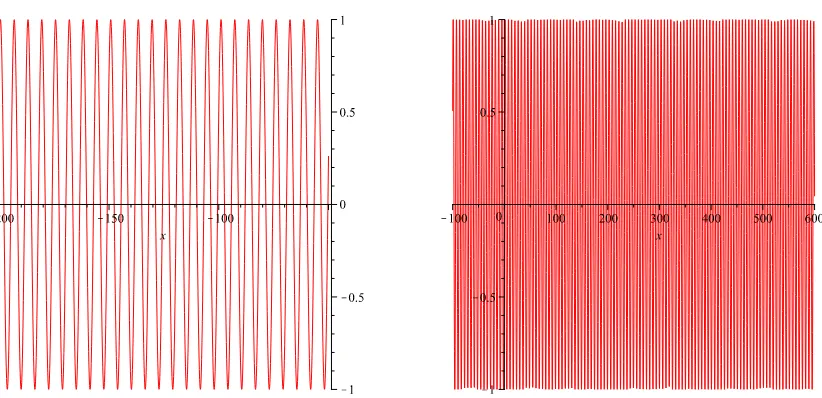
Besides, from (1) with the declaration (2), we derive the graph of piecewise polynomial approximation to the sine function by the commandplot(f(x),x=a..b,numpoints=500). We chose the large valuesr=150 andr=500 for the intervals[−200,−50]and[−100, 600], respectively. Let us try the caser=500 to see the display of 448 pairs of interval-polynomial with the accuracy of 1/10500. The corresponding graphs are depicted in Figure1.

We may also explorePiecewiseFunctfrom the other side of our approximation. We have used Taylor polynomials with larger degrees when higher accuracy required so far. If we want to confine approximate polynomials to a fixed degree, we might relate this determination to the vector spaceP_`, a subspace ofL2(a,b). We know that inP_`there is the best polynomial approximationpbestof the sine function inL2_-norm_{k · k}₌_h·_,_·i1/2

ofL2₍_a_,_b₎_{, which is endowed with the inner product}

hϕ,ψi=

Z b

(9)

Figure 1.The graphs of fwithr=150 (left) andr=500 (right).

Now, we use the Gram-Schmidt procedure to find an orthonormal basis{p0,p1, . . . ,p`}forP`

from the basis{1,x,x2_{, . . . ,}_x`_}_{, according to the recursion}

p0:=1/k1k=1/ √

b−a, qk:=xk− k−1

∑

i=0

hxk,piipi, pk :=qk/kqkk, k=1, . . . ,`. (3)

Once the orthonormal basis has been found, we obtain

pbest=hsin,p0ip0+hsin,p1ip1+· · ·+hsin,p`ip`= `

∑

k=0

hsin,pkipk.

To give an estimate forksin−Fk, whereFis our piecewise polynomial approximation to the sine function on[a,b], we first approximatehsin,pkiby

hsin,pki=

Z b

a pk

(x)sinxdx≈ hF,pki=

Z b

a pk

(x)F(x)dx. These estimates have the absolute error

|hsin,pki − hF,pki|=|hsin−F,pki| ≤ ksin−Fk, where

ksin−Fk=

Z b

a |sinx−F

(x)|2dx1/2≤b−a 102r

1/2

= √

b−a 10r . Therefore, if we choose

pc_best:= `

∑

k=0

hF,pkipk (4)

as an approximation ofpbestthen we have the following estimation for the error norm

kpbest−pcbestk=

`

∑

k=0

hsin−F,pkipk ≤

`

∑

k=0

|hsin−F,pki| ≤ (`+1) √

b−a

(10)

Hence, we may taker=blg((`+1)√b−a)c+1+uto obtain the estimate

kpbest−pcbestk< 1 10u.

To determinepc_bestwith MAPLE, it would be better to write the polynomial pk in the form of pk:=∑ks=0aksxs, hence we have

hF,pki=

k

∑

s=0

akshF,xsi, withhF,xsi=

Z b

a x

s_F₍_x₎_dx₌

_∑

n i=0

Z _α_i₊₁

αi

xsAi(x)dx. (6)

According to the initial settings in (1), the coefficientsaksand the inner productshF,xsican be computed by the following commands

aks→coeff(p[k],x,s)

hF,xsi →add(int(x^s*F[i],x=a[i]..b[i]),i=1..num)

We can make a procedure namedPowerIntApproxonly to computehF,xsi,s = 0, . . . ,`. This procedure that has one more argument, say “deg”, for the chosen degree ofpbestmay take all the blocks ofPiecewiseFunct, but replacing the output of Block 3, Block 4 and the last part ofPiecewiseFunct with the commands recapped in the following. For the outputRETURNof Block 3, we take the sum of integrals ofxsAi(x)on[αi,αi+1], instead of giving the sequence of[αi,αi+1],Ai; and we do similarly for the output of Block 4. The last part ofPiecewiseFunctmay be replaced with the commands

if 0<=a then

evalf[r](ApproxInt(a,b,deg,r));

elif b<=0 then

evalf[r]([seq((-1)^(i+1)*ApproxInt(-b,-a,deg,r)[i+1],i=0..deg)]); else

evalf[r]([seq((-1)^(i+1)*ApproxInt(0,-a,deg,r)[i+1],i=0..deg)]

+ApproxInt(0,b,deg,r)); end if:

and the reason why we do so can be easily recognized. Here, ApproxInt has a similar role to ApproxFunct, but simpler to use.

Now, we have enough materials derived from (3), (4), (5) and (6) to make a procedure for finding a desired approximation on[a,b]inL2-norm to the best approximationpbestof the sine function inP`

with a given positive integer`. The procedure takes four argumentsa,b,ànduto givep∈ P_às its output such thatkp−pbestk<1/10u. As mentioned above, if we named the procedureBestApprox, hence it takesPowerIntApproxas its local variable, then it would be interesting to runBestApprox with different values of its input. But, as warned in Section 1, we should pay much attention to the cases of large values ofànduin order to take an appropriate regulation.

4. Conclusion

There could be some more useful ways to explore the output ofPiecewiseFunctand its corollary, PowerIntApprox, as well asSine. Although these procedures are designed only for the sine function, we can make some appropriate changes to the blocks of commands to obtain their “cosine” version. It is hoped that some application results of our procedures would supply some more improved computational tools in applied mathematics.

(11)

thankfulness to the Maplesoft experts for their great work on developing MAPLE. The paper could not be well illustrated without MAPLE, their powerful and user-friendly product.

Conflicts of Interest:The author declares no conflict of interest.

References

1. Hardy, G.H.; Wright, E.M. (revised by Heath-Brown, D.R.; Silverman, J.H.). An Introduction to the Theory of Numbers; 6th ed.; Oxford University Press: Oxford, UK, 2008.

2. Monagan, M.B.; Geddes, K.O.; Heal, K.M.; Labahn, G.; Vorkoetter, S.M.; McCarron, J.; DeMarco, P.MAPLE Introductory Programming Guide; Copyright cMaplesoft. Waterloo MAPLE Inc.: Ontario, ON, Canada, 2008. 3. Monagan, M.B.; Geddes, K.O.; Heal, K.M.; Labahn, G.; Vorkoetter, S.M.; McCarron, J.; DeMarco, P.MAPLE Advanced Programming Guide; Copyright cMaplesoft. Waterloo MAPLE Inc.: Ontario, ON, Canada, 2008. 4. Muller, J.M.Elementary Functions–Algorithms and Implementation; 2nd ed.; Birkhäuser Boston: New York, NY,

USA, 2006.

5. Niven, I.; Zuckerman, H.S.; Montgomery, H.L.An Introduction to the Theory of Numbers; 5th ed.; John Wiley & Sons, Inc.: New York, NY, USA, 1991.

6. Quan, L.P.; Nhan, T.A. Applying Computer Algebra Systems in Approximating the Trigonometric Functions.