Study and verification of the superposition method used for determining the pressure losses of the heat exchangers

a

Corresponding author: [email protected]

Study and verification of the superposition method used for determining

the pressure losses of the heat exchangers

Michal Petru1,2 a, Petr Kulhavy2, Pavel Srb2 and Gary Rachitsky3

1

Institute for Nanomaterials, Advanced Technologies and Innovation, Technical University of Liberec, Studentská 2, 461 17, Liberec 1, Czech Republic

2

Faculty of Mechanical Engineering, Technical University of Liberec, Studentská 2, 461 17, Liberec 1, Czech Republic 3

Faculty of Mechanical Systems Engineering, Conestoga College, 299 Doon Valley Drive, Kitchener Ontario, Canada.

Abstract. This paper deals with study of the pressure losses of the new heat convectors product line. For all devices connected to the heating circuit of the building, it‘s required to declare a tabulated values of pressure drops. The heat exchangers are manufactured in a lot of different dimensions and atypical shapes. An individual assessment of the pressure losses for each type is very time consuming. Therefore based on the resulting data of the experiments and numerical models, an electronic database was created that can be used for calculating the total values of the pressure losses in the optionally assembled exchanger. The measurements are standardly performed by the manufacturer Licon heat hydrodynamic laboratory and the numerical models are carried out in COMSOL Multiphysics. Different variations of the convectors geometry cause non-linear process of energy losses, which is proportionately about 30% larger for the smaller exchanger than for the larger types. The results of the experiments and the numerical simulations were in a very good conjuncture.Considerable influence of the water temperature onto the total size of incurred energy losses has been proven. This is mainly caused by the different ranges of the Reynolds number depending on the viscosity of the used liquid. Concerning to the tested method of superposition, it is not possible to easily find the characteristic values appropriate for the each individual components of the heat exchanger. Every of the components behaves differently, depend on the complexity of the exchanger. However, the correction coefficient, depended on the matrix of the exchanger, that is suitable for the entire range of the developed product line has been found.

1 Introduction

Currently, across all the industry sectors, there is a main theme of more effective use of resources with respect to the environment. Often, and practically in the all industries sectors, we encounter reduction of volume, weight and power of delivered energy. Their more efficient utilization of both for the final product, and the manufacturing process [1,2]. The next and in some industries somewhat underappreciated sectors is the testing of the products and methods for establishing and controlling their functional parameters. Similarly, going passed through the development of equipment for the heating in buildings. From the original cast iron radiators over time is the move towards a smaller, lighter, and more powerful variants. Today‘s modern radiators can be divided into several parts. These parts are used to ensure functionality and simultaneously delivering to the product his final form. Classic radiators are used for the transmission and transformation of heat into the surroundings through radiation. Modern heating bodies, called convectors use principle of free or forced convection, where the air movement is accelerated by the

fan [3,4]. The heating unit manufacturer is required to declare heat power, pressure loss and acoustic characteristics of fan, namely the sound pressure level. One of the leading Czech producers of heaters that operate on the principle of free and forced convection is the Liberec manufacturer Licon heat s.r.o. a subsidiary company of the Korado group. In common cooperation studies were conducted of the heating convectors mentioned in this article. Generally, heating convectors are designed for the heating in the living spaces, are gradually replacing the classic radiators. The convector operates using a heat exchanger through which air travels, typically with the help of the tangential fan driven by air from the room, as can be seen by Figure 1. The body of the heat exchanger consists of copper tubing that covers the effective area back and forth, connecting fittings and the bleeder valve. The whole bundle of tubes is fitted with the patented aluminum fins to increase the heat output.

At the work, that presented [4] was searching for the energy balance between the heat comfort and overall energy supplied to the room. The research was conducted in order to find the ideal matrix deployment of the most C

Owned by the authors, published by EDP Sciences, 2015

appropriate position of the tubes and fins. The results showed that in energy terms, it is more advantageous that natural convection should be caused by the movement of warm air after heating naturally. Such a solution appears to be preferable, especially in terms of material savings. The usage of the fan, the control and power required for the power supply, directly associate with the end product and overhead cost. When using the forced convection, a significantly higher levels of heat output are achieved and therefore this method is widely preferred. The convector operates using of two operating modes - heating and cooling. The cooling system can be normally used single-circuit when cold liquid is fed in the same way as warm and switching circuit occurs globally throughout the building. The second, less known possibilities is a system with a two circuits where are the both modes completely independent. For a system with two separate circuits, more tubes are required than for the heating system. This compromise is due to logically considering the relatively small temperature gradient generated during cooling (medium temperature recommended approximately ~ 9°) compared with the gradient achieved by heating the heat exchanger in the room air at significantly higher values. The volume of water in the individual types of heat exchangers ranges from 0.18 to 1.2 liters per meter of length and the volumetric flow up to 5 l / min. Thermal output at an ambient temperature 20 °C and the the mode of operation 70/55 ° C reaches the values in the range of 190 to 7800 W. The cooling power reaches values up to 2000 W.

In the studied case, a heat exchanger designed for one primary circuit was used, which has been studied for usability of the FEM and superposition methods for detecting the pressure losses in the convector [1].

Figure 1. Bench convector with forced convection.

2 Introduction into the solved problem

For the whole range of convector models, an assessment of the most appropriate methods for the determination the pressure losses that are arising during the flow of the heating medium through the heat exchanger are required. The pressure drop is necessary to find and determine specification tabulated values, which are provided by the manufacturer of heating systems for designers, installers and customers. From the known pressure loss, average value of temperature the heating medium in the system and the required mass flow rate can be accurately used to set the whole building thermal cycle. This cycle will be the switching pressure and the required power of the pumps. When determining the pressure loss it is necessary to take into account the considerable scatter values operating temperature of the heating medium. The dynamic viscosity of the fluid decreases proportionally in direct dependence on the increasing temperature. The impact of the total pressure in the system is not necessary and can be completely neglected.

2.1 Mechanical properties of water

When a fluid is used in industry, an energy transfer occurs inside the flow. In the case of thermal energy, it is necessary to consider its internal friction and the resulting shear stresses. Not considering the existence of tangential stress is possible only for an ideal fluid, or liquid real, which however does not move as stated in eg. [5-8]. When particles of the fluid start moving, the adjacent particles also begin to move at the same time. The cause of this phenomenon is the velocity gradient dv/dy is increasing the internal friction between the molecules and their thermal motion, which is the particle kinetic energy transmitted to its surroundings. Classical physics talks about cohesion when there is a case of coherence of molecules of the same elements, and adhesion in cases where there is a hold of diverse particles during random encounters [8]. For the dynamic viscosity, it is possible to use the relation according to the equation (1) as shown in [6].

T const d

T m grT

c .

3 2 3

3 1 3

1

2 2 /

3 =

= =

= κ

π ρλ

ρλ

η ,

(1)

where

κ

is the Boltzmann constant, m2 kg s-2 K-1; λ mean free path of the molecules, and m corresponds to the weight of a single molecule.

where the temperature can changes occur in inaccurate or overflow opening. Actual flow of liquid in a closed geometry can be described with using the Navier-Stokes equations, which is essentially a special case of the Cauchy equations of motion a fluid according to (2).

u

u

p

u

f

t

u

&

&

&

&

&

+

∇

+

∇

=

∇

+

∂

∂

1

ν

2

ρ

,

(2)

where

u

&

is the speed,

z

u

y

u

x

u

u

_{x y z}

∂

∂

+

∂

∂

+

∂

∂

=

∇

&

p is the pressure, Pa;

t

is time, s; ν is the kinetic viscosity, m2·s-1 ;and

f

&

is a vector of the volume forces.

2.2 The numerical model for the study of

pressure losses of the heat convector

The numerical model for calculating the pressure loss of the heat convector was carried out in the finite element (FEM) Fluid Dynamics module of COMSOL Multiphysics. COMSOL Multiphysics is suitable for modeling various physical phenomena by electrostatics and electrokinetics through dynamic processes up to the fluid flow and compression of isotropic or anisotropic materials [9].This software includes a number of tools designed to solve a wide range of problems that are described by partial differential equations as specifically in this case used Navier-Stokes equation (2). COMSOL was used to compute the implicit algorithm where at each time instants velocity gradually updated in time t with a time increment t + dt according to equation (3) as opposed to explicit algorithm that is suitable for other types of dynamic analyzes as said Petr#, Novák, Herák and Simanjuntak [10-11].

t t i t t i

i

u

u

u

₊₁

=

₊+₁Δ

−

+Δ

δ

_,

₍₃₎

where

u

_it+Δt is the vector of nodal displacement for the i-iteration in the time t+Δt.

The numerical model allows the modeling of the vector momentum distribution of the fluid flowing in the coil. The results affect the corresponding initial and boundary conditions that are particularly difficult due to the complicated geometry of the heat exchanger, through which flows the driving medium. The boundary conditions were defined the same way as with the real devices, for the selected observed temperature (12, 23, 40 and 60 ° C) and for the selected flow velocity. The input parameters of the numerical model for analysis of the pressure loss are shown in Table 1.

Table 1. The input parameters of the numerical model

a) Dynamic viscosity decreases with the rising temperature

The model itself was based on the modified 3D CAD data model of the heat exchanger with a real dimensional geometry. The suitable variant of the calculation depending on the size of the Reynolds number was chosen in the simulation. This is a laminar flow, turbulent flow with a low Re number called "transitional region" and turbulent flow.

• The Reynolds number

ܴ݁ ൌ

஡ܞ஽_ఎ

ൌ

ܞ஽_జ

ǡ

(4)

where

η

is the dynamic viscosity (1), N·s·m-²; ρ is the density of the fluid, kg·m-3; D is the inner diameter of the round pipe and v is the mean velocity of the fluid, m·s-1.

During the model simulation of process like this, problems arrise in the convergence of solutions. Sometimes the finite solution can despite very sophisticated procedures Gauss elimination iterate with unacceptable error. Therefore, it is necessary already when drawing up the model that there will be close to the real behavior. This suggests a suitable design adaptive finite element mesh that meets the criteria of flow, boundary and initial conditions, etc. These are a primary target in order to appropriate numbers of iterations already in the beginning of the calculation (Figure 2) to a sufficient degree for minimize the resulting residue defined by equation (5). The calculation is shown in Figure 2. and in Table 2. The resulting dependence of the convergence calculation, which is given by the expression, sizes residues and the number of iterations (linear or nonlinear).

[

]

zk z n

k

c

f

z

dz

s

f

z

i

a

= = −

=

³

=

¦

1

1

(

)

Re

(

)

2

1

π

,

(5)

where a-1 is rezidium of the function f (z) at the nodal

point z0 and f(z) represents a function meromorphic Laurent series around the isolated singular point (node), and must pay (z0 & z). Res [f (z)] z = zk is called the rezidium of function f (z) in the k-th nodal point zk.

The temperature of the convector (°C) The inlet pressure p1 (kPa) The flow velocity v1

(m s-1)

Dynamic viscosities a)

(Pa.s) Density

(kg/m3)

Figure 2. Dependence the residues of the numbers of the convergence iterations: nonlinear solution (left), linear solution (right).

When using the adaptive techniques, it may happen that even though the critical threshold will significantly soften, the stiffness matrix becomes badly definite. Therefore the use of the multi-network methods (multigrid method), which essentially combines a finite iterative method [12]. The error of the solution can be divided into singular (local) and global. Singular is the high frequency error that is not locally extensive, but can be reduced with the iterative process. Global low-frequency error, has the nature of a smooth function and affects virtually all of the solutions in the areas. The finite element mesh was therefore created from 3D Solid tetrahedron (10-node elements) with the total numbers of degrees of freedom specified in the Table 2. For a sufficiently and accurate solution in geometrically complex areas (radius, knees), adaptive technique were developed in elements of 0.002 mm size. Detail of the proposed finite element mesh is shown in Figure 3.

Figure 3. The mesh of model for calculating the pressure loss of the inlet part of heat exchanger

Figure 4. FEM model of the easiest kind of exchanger with the straight tubes and inlet / outlet parts.

Figure 5. FEM model of the basic construction part of exchanger with meandr and unilateral inlet/outlet.

Table 2. The values of the resulting finite element mesh

a) _{The required accuracy of the solution is consistent with the solution} by 'e ' error, that is the sum of contributions of individual error components [13,14].

2.3 Experiment

• Prototype parts

Due to the large number of possible assemblies of the heating coil design, it is a time consuming to set values for each type individually. Neglecting the shape or size, the exchanger always consists of four basic elements that give the resulting characteristics of the resulting flow. The individual parts are the Inlet / Outlet, 180° elbows and straight pipe. The basic construction of exchanger matrix consists of the shape of fins that can be freely assembled from the basic shape of the cut aluminum sheet, as is shown in Figure 7. In the real design, typically encountered are the implementation of the matrix from 2×2 to 3×6. The larger version would not increasing their thermal output and therefore are suitable only for multi-circuit systems.

Figure 7. The default matrix of the exchanger aluminium plate.

Were assembled and determined characteristics of the prototype parts individual in the physical form and in the form of the mathematical models. Subsequently, the manufacturer's engineering data was in the form of

contingency tables and macros of VBA_MS_Excel. These created a computational database of all possible versions of the product. Every possible construction variant has therefore in advance clearly the composition of all components and can be easily used to create a CAD model (Figure 8). To calculate the total pressure loss, the user of the database only selects a desired matrix and the length of the exchanger. For each component is numerically or experimentally determined characteristics of the pressure field, depending on the flow rate. The computational database based on the specified input data, using the specific characteristics of each element can calculate the parameters of future devices.

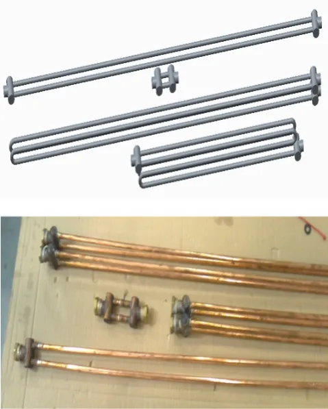
Figure 8. The real models parts (above) and measured prototype parts (below).

• Principle of the experiment

The principle of the experiment (Figure 9,10) was based on the difference in fluid levels in the piezometric tubes to determine the pressure loss. Liquid is pumped with an electronically controlled pump, fed from the tank through the control ultrasonic flowmeter to the heat exchanger. From the outlet of the exchanger is the liquid again returned to the tank. Principle of measurement consists of subtracting the differences of the piezometric tubes levels at the input and output. A measured difference in fluid levels is the known density of water converted to the resulting pressure difference and then to a losses of the specific energy. The measurement was performed for 4-point temperature of water and at variable flow rates 0.1-5 l×min-1 which is joined to the connecting fitting the heat exchanger.

Parts Number

of nodes / elements

The number of iterations nonlinear /

linear

Resid ual value

The required accuracy (%) a)

Inlet

Figure 3.

504/444

3 16 / 204

3.4e-004 5

Straight Figure 4.

2196/17

800 25 / 508

1.2e-005 5

Meandr

Figure 5.

2940/26

542 20 / 342

4.2e-005 5

Exchanger

Figure 6.

7913/64

393 25 / 584

This constitute a speed of approximately from 0.01 to 0.3 m/s. The lowest temperature approximately of 9°C corresponds to the recommended water temperature for cooling. The highest temperature was chosen due to that it was approximately the same steps between the test temperatures to 60°C.

Figure 9. The experimental device and used equipment.

Figure 10. The isolated heat exchanger during the measurement pressure losses with the hot medium.

3 Results and discussion

When comparing the specific energy losses depending on the Reynolds number showed that the FEM model a very good agreement with the experiment (Figure12,13). In Figure 12 is showing a comparison of the values for the temperature of 23°C on the FEM model. It can be concluded that the FEM model works with the calculation error within 5% as is shown in Table 2. The distribution of pressure losses in the construction geometry of the heat exchanger in the FEM model for the flow velocity of

0.2 m/s is at Figure 4-6. It is obvious that with the increasing velocity, the pressure loss increases as well. For the flow velocity of 0.05 m/s, the pressure loss is approximately 400 Pa, but for four times larger velocity of 0.2 m/s it is already approximately 5000 Pa. Therefore there is a significant exponential increase of the pressure loss. In the Figure 11 one can see the relation of the ez (6)

on the actual value of Reynolds number (4) for each temperature 9, 23, 40 and 60°C.

݁

_௭

ൌ

୼௣_ఘ, (6)

where ez is the specific energy losses, J·Kg-1.

Obviously (Figure 11), the maximum specific energy losses are almost identical for higher temperatures in range from 40° to 60°C which is in contrast to the differences of the Reynolds number. In the range of lower temperatures (Re<4000), the variation of temperature leads to significatn change of the energy losses. With increasing temperature, the energy loss continually decreases until it is at almost a constant value. This can be caused by the fact that at higher temperatures, the dynamic viscosity gradually converges to a constant value.

In a real and numerical model, a similar characteristic course and final values arises. Despite this, the values obtained using the calculation in the database based on the principle of superposition, reach large inaccuracies and the resulting pressure losses are higher. This is evident from Figure 12, 13. For each matrix of the assembly, it is possible to determine a correction factor, with which the calculuated values reach an agreement with the actual ones. The results show that the value of the coefficient are not significantly affected by the size of the total length of the exchanger, but only by the base of the matrix number of the tubes and number of peripherals like inlet/ outlet, bends and valves.This makes it possible to use the coefficient for the entire linear range of the specified heat exchanger assembly‘s.

Figure 11. The distribution of specific energy losses in dependence on the Reynolds number and the heat medium temperature.

elements is. For example, for heat exchanger with matrix 12, which may be in the arrangment 3×4 or 2×6, we get practically the same values. The main cause of the increased values with using the method of superposition, will most likely amplifyes the small initial errors and the inability to assess the effects resulting during the transition from one part of the convector to another. Furthermore is necessary to consider that the speed profile changes with the length of coil. In short fittings, the speed profile is entirely different at the end of a long pipe.The total pressure loss could be also affected by the formation of a vortex structures. For example in the elements such as the knees or input elements where there is flow exposed to the rapid changes in cross-section. These are all things that are not adequately taken into account for calculating process based on the superposition, but it is possible to consider them with an additional form of the correction coefficient (Figure 14).

Figure 12. Comparison of the resulting specific energy losses depending on the Reynolds number in the FEM model, superposition method and experiment on the real exchanger 4x3_L120.

Figure 13. Comparison of the resulting specific energy losses depending on the Reynolds number in the FEM model and superposition method on the exchanger 2x2_L280.

Figure 14. The value of the correction coefficient for every possible assembly of the heat exchanger.

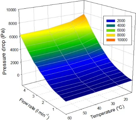
Figure 15. The distribution of pressure losses in the heat exchanger geometry in dependence on the liquid flow velocity and temperature on the real exchanger 4x3_L120.

In Figure 15 is showed the dependence on the pressure losses and the flow rate of the heating medium at the different temperatures. The results in this form are usually provided to designers of the heating circuits. At the last Figure 16 is the comparison of the used methods showed in the above-mentioned dependencies that are the pressure losses and the flow rate.

4 Conlusions

This article dealt with a comparison and assessment of the suitability for use the numerical and experimental analysis for the study of pressure losses in the heat exchanger of the convector, which is typically used for heating or cooling in buildings. The compiled FEM model was in very good agreement with the experiment as shown in comparisons (Figure 12). The specific energy losses are logically the highest at the low values of Reynolds number and with higher flow rates.

The dependence of the specific energy losses on the value of the Re for each temperature 9, 23, 40 and 60°C, is indicated in the graph in Figure 11. There is a characteristic that for the higher temperatures of 40 and 60°C, the maximal energy lossesare almost identical. In contrast to lower temperatures where the increase of energy loss is significant. It is evident that, particularly at low water temperatures there is a considerably affected flow rate and energy or pressure loss. With increasing temperature, however, the temperature effect on the pressure drop continually decreases until it reaches a constant value, which may be caused by the fact that at higher temperatures the dynamic viscosity gradually converges to a constant value.

These results are important for the correct dimensioning of heating systems and to assess the appropriateness of the use of heat convectors for heating a buildings. Also for assessment of the significance and the correlation influence the water temperature on the total dimensioning the system pressure.

A method based on the physical principle of superposition was designed and verified. The principle of superposition permits to determine the characteristic behaviour (depending on the pressure drop, flow rate, Re and temperature) for all of the heat exchanger individual components. Further, all the contributions from the heat exchanger individual components were summed up with the use of MS Excel interactive Visual Basic database based on the principle of contingency tables. Applying a correction factor, which was calculated from experimental and simulated data, the method is sufficiently reliable and accurate.

Acknowledgements

We give our thanks to the construction department and management of the company Licon heat s.r.o. for the provided information.

This work was supported by the Ministry of Education of the Czech Republic within the SGS project no. 21007 on the Technical University of Liberec.The results of this project LO1201 were obtained through the financial support of the Ministry of Education, Youth and

Sports in the framework of the targeted support of the "National Programme for Sustainability I" and the OPR&DI project Centre for Nanomaterials, Advanced Technologies and Innovation CZ.1.05/2.1.00/01.0005 and Project OP VaVpI Centre for Nanomaterials, Advanced Technologies and Innovation CZ.1.05/2.1.00/01.0005 and by the Project Development of Research Teams of R&D Projects at the Technical university of Liberec CZ.1.07/2.3.00/30.0024

References

1. P. Kulhavy, M. Petru, P. Srb, G. Rachitsky,

Manufactruing Technology (to be published 2015)

2. M. Petr#, Novák, O. Šev>ík, L., P. Lepšík, Applied Mechanics and Materials, 157, (2014)

3. LICON HEAT s.r.o., Sm?rnice technologie a konstrukce. (Liberec, 2014)

4. K. Frana, Engineering and Technology, 6, (2012)

5. F. Lemfeld, Journal of Applied Science in the Thermodynamics, (2011)

6. S. Drábková, Mechanika tekutin. Ostrava: VŠB - Technická univerzita, (2007)

7. J. Janalík, Viskozita tekutin a její mení. VŠB Ostrava, (2010)

8. L. DvoQák, Vlastnosti tekutin. VŠB Ostrava, (2010)

9. M. Petr#, O. Novák, P. Lepšík, Applied Mechanics and Materials, 217, (2014)

10. M. Petr#, O. Novak, D. Herak, S. Simanjuntak, Biosystems Engineering, 412(4), (2012)

11. M. Petr#, O. Novak, D. Herak, S. Simanjuntak, 127 , Biosystems Engineering, (2014)

12. M. Petr#, O. Novák, P. Lepšík, Applied Mathematics, 5a, (2013)

13. R. Wienands, W. Joppich, Practical Fourier Analysis for Multigrid Methods, Chapman & Hall/CRC, 217, (2005)

14. Chen, Zhangxin, Guanren Huan a Yuanle MA.