Evolution of the ALICE Software Framework for Run 3

(1)

Evolution of the ALICE Software Framework for Run 3

GiulioEulisse1,∗_,_Piotr_Konopka2,1_,_Mikolaj_Krzewicki3,4_,_Matthias_Richter5_,_David_Rohr1_, andSandroWenzel1

1_{Organisation Européenne pour la Recherche Nucléaire, CERN, Meyrin, Switzerland}

2_{Akademia Górniczo-Hutnicza im. Stanisława Staszica, AGH University of Science and Technology,} Kraków, Poland

3_{Frankfurt Institute for Advanced Studies, Frankfurt, Germany} 4_{Johann-Wolfgang-Goethe University, Frankfurt, Germany} 5_{University of Oslo, Oslo, Norway}

Abstract.ALICE is one of the four major LHC experiments at CERN. When

the accelerator enters the Run 3 data-taking period, starting in 2021, ALICE expects almost 100 times more Pb-Pb central collisions than now, resulting in a large increase of data throughput. In order to cope with this new challenge, the collaboration had to extensively rethink the whole data processing chain, with a tighter integration between Online and Offline computing worlds. Such a system, code-named ALICE O2_{, is being developed in collaboration with the} FAIR experiments at GSI. It is based on the ALFA framework which provides a generalized implementation of the ALICE High Level Trigger approach, de-signed around distributed software entities coordinating and communicating via message passing.

We will highlight our efforts to integrate ALFA within the ALICE O2 ronment. We analyze the challenges arising from the different running envi-ronments for production and development, and conclude on requirements for a flexible and modular software framework. In particular we will present the AL-ICE O2_{Data Processing Layer which deals with ALICE specific requirements} in terms of Data Model. The main goal is to reduce the complexity of develop-ment of algorithms and managing a distributed system, and by that leading to a significant simplification for the large majority of the ALICE users.

1 ALICE Experiment in Run 3

The Large Hadron Collider (LHC) will undergo a major technical stop between 2018 and 2020, which will result in five fold increase in the heavy ion rate that will go from the current 10kHz to the planned 50kHz. Due to this upgrade the ALICE experiment [1], which of the four major experiments at the LHC is the one particularly focused on the heavy-ion physics, will undergo a similar major upgrade to cope with increased number of collisions [2].

A major difference from the current setup is that, because of the high latency of gas

detectors like the Time Projection Chamber (TPC), it will be impossible to sustain the current (O(1kHz)) triggered mode, instead data will be collected with continuous readout mode.

(2)

FLP

EPN

FLP

Detector

EPN

≳3TB/s up to 500GB/s

...

ReadOut

Synchronous 

reconstruction 

(data reduction)

On-site 

storage

EPN / Grid

...

Asynchronous  reconstruction  (improved conditions)

EPN / Grid

EPN / Grid Permanent  storage

up to  100GB/s

EPN input data quantum is the "timeframe": 23ms of continuous

readout data. ~10GB

EPN_EPN_EPN EPN

BEAM ON: data reduction _{BEAM OFF: improved calibration}

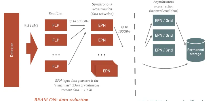
Figure 1.The Computing architecture of ALICE in Run 3

The total throughput from the detector will increase up to 3 TB/s, to be then reduced to

500 GB/s after initial compression by a farm of consisting in about 150 parallel First Level

Processors (FLP) computing nodes. Raw data will be split in chunks, so called “uncom-pressed timeframe”, up to 23 ms long. As seen in figure 1, a many-to-many network setup will then recompose all the parts belonging to the same timeframe on one of the Event Pro-cessing Nodes (EPN) in a round robin manner. Each timeframe will be in average 10 GB in size and each EPN is expected to perform reconstruction on it and use the derived quantities (e.g. track parameters) as a mean to compress raw data related information and reduce the size of each “compressed timeframe” to an average of 2 GB with an aggregate rate of 100 GB/s to persistent storage. A later asynchronous (to data taking) step will then use the EPN

farm to reprocess all the data taken in the synchronous processing, using final calibrations and reconstructing the part of the detectors that can afford late reconstruction.

A major difference between Run 3 and the Run 1–Run 2 data processing is therefore the

blending of traditional roles of Online and Offline, which will actually share the exact same

algorithms.

2 ALICE O

2

_Framework

In order to cope with the challenges of Run 3 and in particular to ensure components reusage between the synchronous and asynchronous phases, ALICE is developing a new Software

framework, dubbed O2_{[3, 4], in collaboration with the FAIR Software Group at GSI. ALICE}

O2_{architecture derives from the current (Run 1, Run 2) architecture of the ALICE High Level} Trigger (HLT) [5] and can be considered subdivided in three major parts:

• The Transport Layer, FairMQ

• The O2_{Data Model}

(3)

FLP FLP EPN FLP Detector EPN EPN

≳3TB/s up to 500GB/s

...

ReadOut Synchronous  reconstruction  (data reduction) On-site  storage

EPN / Grid

...

Asynchronous  reconstruction  (improved conditions)

EPN / Grid

EPN / Grid Permanent  storage

up to  100GB/s

EPN input data quantum is the "timeframe": 23ms of continuous

readout data. ~10GB

EPN_EPN_EPN EPN

BEAM ON: data reduction _{BEAM OFF: improved calibration}

Figure 1.The Computing architecture of ALICE in Run 3

The total throughput from the detector will increase up to 3 TB/s, to be then reduced to

500 GB/s after initial compression by a farm of consisting in about 150 parallel First Level

Processors (FLP) computing nodes. Raw data will be split in chunks, so called “uncom-pressed timeframe”, up to 23 ms long. As seen in figure 1, a many-to-many network setup will then recompose all the parts belonging to the same timeframe on one of the Event Pro-cessing Nodes (EPN) in a round robin manner. Each timeframe will be in average 10 GB in size and each EPN is expected to perform reconstruction on it and use the derived quantities (e.g. track parameters) as a mean to compress raw data related information and reduce the size of each “compressed timeframe” to an average of 2 GB with an aggregate rate of 100 GB/s to persistent storage. A later asynchronous (to data taking) step will then use the EPN

farm to reprocess all the data taken in the synchronous processing, using final calibrations and reconstructing the part of the detectors that can afford late reconstruction.

A major difference between Run 3 and the Run 1–Run 2 data processing is therefore the

blending of traditional roles of Online and Offline, which will actually share the exact same

algorithms.

2 ALICE O

2

_Framework

In order to cope with the challenges of Run 3 and in particular to ensure components reusage between the synchronous and asynchronous phases, ALICE is developing a new Software

framework, dubbed O2_{[3, 4], in collaboration with the FAIR Software Group at GSI. ALICE}

O2_{architecture derives from the current (Run 1, Run 2) architecture of the ALICE High Level} Trigger (HLT) [5] and can be considered subdivided in three major parts:

• The Transport Layer, FairMQ

• The O2_{Data Model}

• The Data Processing Layer

2.1 The Transport Layer: FairMQ

The so called “Transport Layer” is implemented using the FairMQ [6] message passing

toolkit developed at GSI. It defines the core building blocks of the architecture in terms of so

calledFairMQDevices(devices), and implements how they communicate among each other.

This allows to abstract away from the user the interaction with the network fabric itself, which can be either Ethernet, InfiniBand or a mixture of the two. Moreover for the case in which two devices work on the same node, shared-memory-backed message passing is also supported. Effectively FairMQ is an implementation of theactor model[7] for concurrent processing.

2.2 The O2_{Data Model}

On top of the Transport Layer, ALICE builds the “O2_{Data Model” (Data Model), an ALICE}

specific description of the messages being exchanged by the various devices. The Data Model is designed with three key features in mind: being computer language agnostic, being exten-sible, and allowing for efficient transport between nodes and mapping of the data objects in

shared memory or to the GPU memory where required.

Each message is expected to be composed by two parts, a header and a payload. The header by default contains information like the data origin (i.e. the detector or process creat-ing it) a mnemonic data description (i.e. the type of data contained in the payload) and other ancillary information like a spatial index or the serialization method used to encode the pay-load. While a base header is required for every message, user code can attach extra headers allowing the construction of a veritable type system to describe the payloads.

Multiple data formats and serialization methods are supported for the different payloads.

For example, for actual detector data, and in particular for TPC reconstruction, a custom compressed, directly addressable data structure will be utilized.

For all the cases where serialization of complex objects can be afforded, e.g. for Quality

Control and Assurance, native serialization of C++objects, e.g. histograms, is assured via a

native ROOTTMessageserialization.

For data analysis multiple solutions are being investigated, as more deeply discussed in [8]. Besides the above mentioned ROOT ability, one of particular interest is the integra-tion with Apache Arrow [9]. Apache Arrow is a cross-language development platform for in-memory data, providing libraries to do zero-copy streaming messages and interprocess communication. Apart from the technical merits of Arrow which make it a good fit for the O2 architecture, the interesting feature is the large convergence of the Opensource and commer-cial data analysis industry to back Arrow as lingua franca for interoperability between tools like Pandas[10], Spark[11], Parquet[12], and many others. The hope is that by integrating O2 with Arrow we will be able to profit from such a large ecosystem. In this scenario,

compat-ibility with ROOT will be guaranteed by using theTArrowDSdata source, co-developed by

ALICE and the ROOT team, which allows using Arrow withTDataFrame[13].

2.3 The Data Processing Layer

(4)

the devices required to perform a given computation, making sure there are no pathological cases in the configuration like missing or circular dependencies between modules. She would need to keep track of all the in-flight parts relative to a computation, potentially coming from different sources, and dispatch the computation only when all the inputs are available.

To simplify the life of the end user, a third layer, named“Data Processing Layer”(DPL), has been introduced, which allows to describe computation as a set of data processors implic-itly organized in a logical dataflow describing how data is transformed.

The DPL configuration is expressed by the user in a declarative and implicit manner. Each data processor needs to declare upfront its input types (e.g. clusters) as well as its outputs (e.g. tracks). The DPL will create a topology that will connect the producer of some kind of data to all of its consumers. This removes from the user the burden of managing the topology, allows the composition of smaller workflows into larger ones, and leaves to the framework the role of optimizing the logical dataflow description to a physical topology. This approach is similar to what done, in a different context, by tools like Tensorflow [14].

The user implements such dataflow description by providing a callback that fills the model representing the workflow. A simple, self contained, example describing and starting a di-amond shaped workflow of 4 data processor is provided in the listing 1. While the current implementation is available only via the C++API, the model itself is meant to be language

agnostic. Support for other languages or interactive construction in a GUI is foreseen.

#include"Framework/runDataProcessing.h"

using namespace o2::framework;

AlgorithmSpec source() {

return AlgorithmSpec{

[](ProcessingContext &ctx) {

auto aData = ctx.outputs().make<int>(OutputRef{ "a1"}, 1);

auto bData = ctx.outputs().make<int>(OutputRef{ "a2"}, 1);

}}; }

AlgorithmSpec simplePipe(std::stringconst &what) {

return AlgorithmSpec{ [what](ProcessingContext& ctx) {

autobData = ctx.outputs().make<int>(OutputRef{what}, 1);

} }; }

AlgorithmSpec sink() {

return AlgorithmSpec{ [](ProcessingContext&) {} };

}

WorkflowSpec defineDataProcessing(ConfigContext const&specs) {

return WorkflowSpec{

{ "A", Inputs{}, {OutputSpec{{"a1"},"TST", "A1"}, OutputSpec{{"a2"},"TST", "A2"}}, source()}, { "B", {InputSpec{"x", "TST", "A1"}}, {OutputSpec{{"b1"},"TST", "B1"}}, simplePipe("b1")}, { "C", {InputSpec{"x", "TST", "A2"}}, {OutputSpec{{"c1"},"TST", "C1"}}, simplePipe("c1")}, { "D", {InputSpec{"b", "TST", "B1"}, InputSpec{"c", "TST", "C1"}}, Outputs{}, sink()} };

}

Listing 1. A self contained sample of DPL configuration, spawning 4 different FairMQDevices exchanging messages in a diamond topology. When run in laptop mode the Debug GUI provides insights about the running topology.

(5)

the devices required to perform a given computation, making sure there are no pathological cases in the configuration like missing or circular dependencies between modules. She would need to keep track of all the in-flight parts relative to a computation, potentially coming from different sources, and dispatch the computation only when all the inputs are available.

To simplify the life of the end user, a third layer, named“Data Processing Layer”(DPL), has been introduced, which allows to describe computation as a set of data processors implic-itly organized in a logical dataflow describing how data is transformed.

The DPL configuration is expressed by the user in a declarative and implicit manner. Each data processor needs to declare upfront its input types (e.g. clusters) as well as its outputs (e.g. tracks). The DPL will create a topology that will connect the producer of some kind of data to all of its consumers. This removes from the user the burden of managing the topology, allows the composition of smaller workflows into larger ones, and leaves to the framework the role of optimizing the logical dataflow description to a physical topology. This approach is similar to what done, in a different context, by tools like Tensorflow [14].

The user implements such dataflow description by providing a callback that fills the model representing the workflow. A simple, self contained, example describing and starting a di-amond shaped workflow of 4 data processor is provided in the listing 1. While the current implementation is available only via the C++API, the model itself is meant to be language

agnostic. Support for other languages or interactive construction in a GUI is foreseen.

#include "Framework/runDataProcessing.h"

using namespace o2::framework;

AlgorithmSpec source() {

returnAlgorithmSpec{

[](ProcessingContext &ctx) {

auto aData = ctx.outputs().make<int>(OutputRef{"a1" }, 1);

auto bData = ctx.outputs().make<int>(OutputRef{"a2" }, 1);

}}; }

AlgorithmSpec simplePipe(std::stringconst &what) {

returnAlgorithmSpec{ [what](ProcessingContext& ctx) {

autobData = ctx.outputs().make<int>(OutputRef{what}, 1);

} }; }

AlgorithmSpec sink() {

returnAlgorithmSpec{ [](ProcessingContext&) {} };

}

WorkflowSpec defineDataProcessing(ConfigContext const&specs) {

returnWorkflowSpec{

{ "A", Inputs{}, {OutputSpec{{"a1"},"TST", "A1"}, OutputSpec{{"a2"},"TST", "A2"}}, source()}, { "B", {InputSpec{"x", "TST", "A1"}}, {OutputSpec{{"b1"}, "TST", "B1"}}, simplePipe("b1")}, { "C", {InputSpec{"x", "TST", "A2"}}, {OutputSpec{{"c1"}, "TST", "C1"}}, simplePipe("c1")}, { "D", {InputSpec{"b", "TST", "B1"}, InputSpec{"c", "TST", "C1"}}, Outputs{}, sink()} };

}

Listing 1. A self contained sample of DPL configuration, spawning 4 different FairMQDevices exchanging messages in a diamond topology. When run in laptop mode the Debug GUI provides insights about the running topology.

Once a dataflow is described, the user can run it by simply starting a single executable, called the DPL driver. Depending on the deployment environment such a driver will map the dataflow to a concrete topology and from there to a set of processes running FairMQ devices. While doing so, it makes sure the configuration matches the deployment environment. For example, on a laptop it will use a simple debug GUI to display logs and metrics aggregated during the processing. On the other hand, when deployed in the Online Cluster it will make

sure it connects to the production logging and monitoring infrastructure. Once the configura-tion to be deployed is fully determined, the driver will either launch the processes itself (e.g. when running on the laptop) or generate a configuration for third party deployment tools like DDS or the ALICE O2_{Control System [15].}

2.4 Processing inside the DPL

Besides implementing the concrete FairMQ topology from the dataflow definition, the goal of the DPL is to hide (and resolve) most of the complexity and challenges of a distributed system from the person who wants to write a data processing algorithm.

The DPL is designed to be a simplified reactive system, where the user sees data as multiple streams of events being pushed to her, each event with some timestamp attached. She subscribes to one or more streams, and her callback gets invoked when all the synchronous events for the subscribed streams are available. This hides from the algorithm writer the asynchronous behavior of the backing message passing system and it allows the system to gracefully handle back pressure and to model experiment condition data as inputs that are valid for more than one invocation.

The DPL also provides a unified API to handle out-of-band services, like sending metrics to a monitoring back-end, integration with a persistent logging infrastructure and connecting to non-DPL devices.

2.5 Examples of using the DPL

Work is ongoing to describe all steps of ALICE data processing in Run 3 in terms of DPL workflows and we expect that anything related to data processing will be ported to it by the start of Run 3.

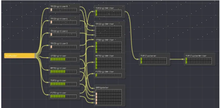
In particular, we have a DPL workflow which describes the digitization process of seven subdetectors out of eleven for of ALICE in Run 3, taking input from a ROOT file produced by the simulation step and producing in output ROOT files with the digits for each detector. This is particularly significant because the actual code was provided by detector experts outside the Framework team and shows that the DPL is already mature enough for wider audience usage within the experiment. A simplified setup with only five detectors, with four parallel workers for the TPC, is show in figure 2.

For the specific case of the TPC, the detector responsible for the largest amount of data in Run 3, the reconstruction chain of the digits produced by the above mentioned workflow has also been implemented in terms of a DPL workflow demonstrating the full end-to-end chain for that detector. This is particularly significant because it also showcases parallel reconstruction of the data, on a sector by sector basis.

DPL has also been used as scaffolding for non strictly data-processing related tasks like

Data Sampling and Quality Control. This in particular demonstrated the ability of DPL to model non data triggered inputs like asynchronous timers.

One of the next steps will be to allow users to combine different workflow seamlessly,

without having to have a top level workflow definition, or out of band communication like a file.

3 Conclusions and future work

(6)

Figure 2.Digitization workflow on-going as shown in the topology viewer of debug GUI, running on laptop

In the future, work will concentrate on the integration with the ALICE Online Control system, on the optimization of DPL produced topologies on different deployment targets and

providing tools that allow end-physicists to write their analysis as part of a DPL workflow.

References

[1] The ALICE Collaboration, Journal of Instrumentation3, S08002 (2008)

[2] The ALICE Collaboration, Journal of Physics G: Nuclear and Particle Physics 41,

087001 (2014)

[3] P. Buncic, M. Krzewicki, P. Vande Vyvre,Technical Design Report for the Upgrade of

the Online-Offline Computing System(2015)

[4] Aliceo2group/aliceo2: First stable release (2018), https://doi.org/10.5281/ zenodo.1493334

[5] D. Rohr, M. Krzwicki, H. Engel, J. Lehrbach, V. Lindenstruth (ALICE),Improvements

of the ALICE HLT data transport framework for LHC Run 2., inProceedings 22nd International Conference on Computing in High Energy and Nuclear Physics(2017), Vol. 898, p. 032031. 8 p

[6] M. Al-Turany, D. Klein, A. Manafov, A. Rybalchenko, F. Uhlig,Extending the FairRoot

framework to allow for simulation and reconstruction of free streaming data(2014),

Vol. 513, p. 022001,http://stacks.iop.org/1742-6596/513/i=2/a=022001

[7] C. Hewitt, P. Bishop, R. Steiger,A Universal Modular ACTOR Formalism for Artificial

Intelligence, inProceedings of the 3rd International Joint Conference on Artificial Intel-ligence(Morgan Kaufmann Publishers Inc., San Francisco, CA, USA, 1973), IJCAI’73,

pp. 235–245,http://dl.acm.org/citation.cfm?id=1624775.1624804

[8] D. Berzano, R. Deckers, C. Grigoras, M. Floris, P. Hristov, M. Krzewicki, M.B.

Zim-mermann, The ALICE Analysis Framework for LHC Run 3, in Proceedings of 23rd

Computing in High Energy Physics(2018), CHEP2018

[9] The Apache Arrow team,From the apache arrow wiki: Physical memory layout(2016),

(7)